Air Quality in Ningbo and Transport Trajectory Characteristics of Primary Pollutants in Autumn and Winter

Abstract

By using meteorology and pollution observation data from Zhejiang province, and data from the National Centers for Environmental Prediction’s Global Data Assimilation System from 1 June 2013, to 31 May 2016, we analyzed air quality characteristics in Ningbo and applied the HYSPLIT model to do backward trajectory clustering statistics for pollution cases of moderate, heavy and severe (henceforth referred to as moderate-and-above) levels. The results indicated that the percentage of moderate-and-above pollution was approximately 6%, which mostly occurred from November to February, with the primary pollutant being particulate matter with a diameter of ≤2.5 μm; Moderate-and-above pollution was mainly caused by pollutants from three types of trajectories (type mx, type 1, and type 2), with type 2 differing significantly from types 1 and mx. Type 2 occurred in stable boundary layers, whereas types mx and 1 occurred in unstable and conditionally unstable layers respectively. These three trajectory types were all related to cold air, but type 2 was weaker than the other two. Analysis of typical cases of various pollution types revealed that a heavy pollution outbreak was due to continuous superposition of pollutants. The input particles most likely originated from the northwest. The upstream situation was the focus of investigation to assist in local pollution forecasting.

1. Introduction

Air pollution index analysis has indicated that air pollution in China is most severe in winter and mildest in summer, with gradual deterioration of air quality from south to north and from coastal to inland regions [1]. Increasing aerosol concentration is the main cause of air quality deterioration and increased haze frequency [2]. In addition, aerosol also affects visibility, cloud formation, precipitation, regional climate, and even human health by altering the nucleus and energy balance [3,4,5,6,7,8,9]. In 2013, the annual average concentration of particulate matter with a diameter of ≤2.5 μm (PM_2.5) reached 72.71 μg m⁻³ in China, whereas it was only 13 μg m⁻³ in the United States [10]. In 2012, the annual average PM_2.5 concentrations in five cities in the European Mediterranean Basin were 14–37 μg m⁻³ [11]. In recent years, China has made considerable efforts to improve its air quality; thus, the annual average PM_2.5 concentration decreased to 47 μg m⁻³ in 2016 (http://politics.people.com.cn/n1/2017/0105/c1001-28999347.html). To set a standard for evaluating the impact of aerosols on health, the European Study of Cohorts for Air Pollution Effects Project was launched to observe PM_2.5 and particulate matter with a diameter of ≤10 μm (PM₁₀) simultaneously in 20 regions in Europe [12], while efforts were made to reduce air pollution to levels that do not endanger human health [13].

Local emissions and external transport cause air pollution. The atmospheric diffusion capability is crucial in the regional transport of aerosols and greatly depends on meteorological conditions. Numerical simulations and the HYSPLIT trajectory method have been used extensively in pollution analysis and research [14,15,16,17,18,19]. Stein et al. [20] detailed the historical evolution and recent improvements in HYSPLIT. Studies of typical pollution cases using combinations of HYSPLIT and mesoscale models have revealed causes of pollution outbreaks in various regions from multiple perspectives [21,22,23,24,25]. Furthermore, analyses yielding backward trajectory statistics have provided useful information. Based on analysis of pollution features and meteorological factors influencing a rare color haze episode in Nanjing in December 2015, Liu et al. [26] discussed the possible reasons and used the HYSPLIT model to analyze the pollution transportation of this purple haze. Lu et al. [27] analyzed the optical characteristics of aerosol particles in central China by using Cloud–Aerosol Lidar observation data and the HYSPLIT model.

In winter, northerly winds prevail in China’s Zhejiang province and transport pollutants southward, while coastal areas have better self-purification capability and thus better air quality than inland areas [28]. Ningbo, located on the coast of northern Zhejiang province (“Zhebei” hereafter), is the second largest city in the province and is representative of coastal cities in Zhebei. Its location is denoted by the cross marked “NB” in Figure 2. Air quality forecasting and services in coastal cities in Zhebei can be obtained through analysis of air quality characteristics and pollutant trajectory statistics in Ningbo. Thus far, few studies have focused on the characteristics of meteorological elements or backward trajectories of aerosol particles in Zhebei.

2. Data and Methods

In China, ambient air quality standards [29] were implemented on 1 January 2016. Typically, air quality is determined based on the air quality index (AQI) of primary pollutants. According to the standards, air quality is classified into six levels: AQI ≤ 50 (excellent), 50 < AQI ≤ 100 (good), 100 < AQI ≤ 150 (slight pollution), 150 < AQI ≤ 200 (moderate pollution), 200 < AQI ≤ 300 (heavy pollution), and AQI > 300 (severe pollution).

The present study period was 1 June 2013, to 31 May 2016, covering 1067 days. The data in this study included the daily valid AQI, daily to hourly concentrations of six major pollutants (PM_2.5, PM₁₀, SO₂, NO₂, CO, and O₃) from the Environment Monitoring Center of Ningbo, and daily to hourly Automatic Weather Station (AWS) observations from the Zhejiang Meteorological Information Center. These data were quality controlled before being entered into the database; thus, missing data were not manually supplemented. Global Data Assimilation System (GDAS) data from the U.S. National Centers for Environmental Prediction (NCEP) networks were also used (ftp://arlftp.arlhq.noaa.gov/pub/archives/gdas1).

3. Air Quality Characteristics in Ningbo from 2013 to 2016

Figure 1a illustrates the percentages of air quality levels (e.g., excellent and good) in Ningbo. The percentages of excellent and good levels were approximately 16.1% and 63.4%, respectively; that is, of the 1067 days, excellent and good air quality were noted on 172 and 676 days, respectively. Furthermore, the percentages of slight, moderate, and heavy/severe pollution were 14.5%, 4%, and 2%, respectively. Thus, the percentage of moderate-and-above pollution was approximately 6% (i.e., 64 days out of 1067 days).

The percentage of each air quality level varied by month (Figure 1b). The excellent level demonstrated a unimodal distribution; air quality peaked in August (23.8%) and increased to the second highest level in July (>20%). Approximately 71% of the excellent levels observed occurred from June to September, whereas only 7.6% occurred from December to February of the following year (henceforth defined as December to February). Among all levels, the percentage of the good level changed the least; it was high in March, April, and October, accounting for 10.2%, 10.9%, and 10.1%, respectively. The monthly variation in the percentage of slight-and-above (including slight, moderate, heavy, and severe levels, used similarly henceforth) pollution was U shaped; the higher the pollution level, the wider was the lower half of the U-shaped curve. For slight pollution, the percentages from June to September were <2%, whereas those from November to February were >10%, totaling 64.5% for these four winter months. For moderate pollution, 93% occurred in these four months. All heavy pollution occurred from December to February, of which 93.3% occurred in December and January. Severe pollution occurred in December for only five days.

Primary pollutant analysis (Figure 1c) indicated that for slight pollution, 78.1% of the primary pollutant was PM_2.5, followed by O₃ (12.3%). Occasionally, PM₁₀ and NO₂ also led to slight pollution. For moderate and heavy pollution, the primary pollutant was PM_2.5, but PM₁₀ was observed as the primary pollutant for two of the five severe pollution days, with the individual AQI (IAQI) of PM₁₀ being as high as 420 and 500 respectively. The IAQI of PM_2.5 also reached 419 and 472 respectively on those two days. Therefore, the primary pollutants for moderate-and-above pollution were aerosol particles, mainly PM_2.5.

The percentages of primary pollutants demonstrated considerable monthly variations according to air quality levels (Figure 1d). For the good level, the percentage of each primary pollutant did not exceed 5% in any month; in other words, no pollutant was a leading cause of pollution. For slight-and-above pollution, the primary pollutant from January to March and October to December was PM_2.5, with >7.1% in all months and >16% in December and January. Moderate pollution mostly occurred in December and January, with PM_2.5 as the primary pollutant, accounting for >25% in all months.

Figure 2 illustrates the average distribution of automatic visibility in Zhejiang over 64 moderate-and-above pollution episodes. During these episodes, visibility was mostly <5000 m in the coastal and inland regions of Zhebei; <3000 m in Hangzhou (HZ), Jiaxing (JX), and Shaoxing (SX); and <2000 m in some local regions. The average relative humidity on pollution days was <80%, with the average maximum relative humidity being <93%. A logical inference is that low visibility was mainly caused by haze (including dry and damp haze). Therefore, when moderate-and-above pollution occurred in Ningbo, slight haze with visibility of <5000 m was common across Zhebei, moderate haze was found inland, and heavy haze occurred on a regional scale.

Figure 3 illustrates the average hourly IAQI evolutions of six major pollutants for the 64 moderate-and-above pollution cases from 2 days before the outbreak (day −2 and day −1) until the occurrence day (day 0) in Ningbo. It shows that PM_2.5 held the highest IAQI, followed by PM₁₀, with IAQI of the other 4 pollutants greatly lower than the above two. The IAQI of PM₁₀ and PM_2.5 were high, with IAQI of PM_2.5 generally >100 two days before the outbreak of the moderate-and-above pollution events. This indicates that not only high levels of PM₁₀ and PM_2.5, but also poor atmospheric diffusion capacities should both be blamed for the pollution occurrence.

4. Clustering Analysis and Statistical Characteristics of Backward Trajectories

4.1. Clustering Analysis of Backward Trajectories for Moderate-and-Above Pollution

During the analysis period, 61 (95%) of the 64 moderate-and-above pollution episodes in Ningbo occurred from November to February, with aerosol particles as the primary pollutants. The HYSPLIT model was used for backward trajectory clustering analysis of these 61 episodes, with the analysis period comprising the day of the pollution outbreak and the day prior to it, totaling 48 h. The start time was set to 23:00 h (China Standard Time) on the day of the pollution outbreak. The start point was set to the Environment Monitoring Center of Ningbo (29.851°N, 121.524°E). Because air pollution mainly occurs in the boundary layer, four heights above ground level (AGL) were set for each pollution episode: 1000, 500, 200, and 50 m. To analyze the characteristics of horizontal transport and deposition of aerosols at various heights within the boundary layer, we tracked the −48 h backward trajectories at each height for each episode and yielded a total of 4 × 61 = 244 trajectories. The critical value of the space variance rate and the number of broad categories were set to 30% and four, respectively.

Figure 4 illustrates the −48 h average backward trajectories of the particles. Approximately 50% of the particles originated from the northwest within 1000 km of Ningbo (trj1), whereas approximately 27% originated from the vicinal areas within 200 km of Ningbo (trj2) and the −42 to 0 h particles of trj2 convoluted within 100 km from the start point. Trj3 and trj4 equally accounted for approximately 11% of the pollution episodes but had different source regions. The −48 h source of trj3 was located in Western China, approximately 1400 km western of Ningbo, whereas trj4 represented long-range transport from 2000 km northwest of Ningbo. The −48 h average heights of trj1 and trj2 were lower than those of trj3 and trj4. Moreover, trj1 and trj2 were below 1500 m with average end heights of 360 m, whereas trj3 and trj4 were above 2500 m with average end heights of 685 m. Thus, 77% of the −48 h aerosols that caused moderate-and-above pollution were located within 1000 km northwest of Ningbo; approximately 27% of these were related to close-range transport within 200 km with an average height of <1500 m; and these aerosols mainly affected air quality in the lower boundary layer. By contrast, approximately 22% of the −48 h pollutant particles originated remotely from a distance of >1400 km with an average height of >2500 m. Through upper transport and deposition, these particles mainly affected air quality in the upper and middle boundary layers above 600 m.

The upper and lower trajectories for each pollution episode may not have been identical. Thus, we defined pollution type 1 as four layers of trajectories identical to trj1 in Figure 4; pollution types 2, 3, and 4 were defined in a similar manner. Type mx was defined as four layers of trajectories that differed from one another.

Table 1. The number of pollution episodes by type and level.

Types	Moderate	Heavy	Serious	Total
type mx	18	9	2	29
type 1	17	3	0	20
type 2	5	3	3	11
type 3	0	1	0	1
type 4	0	0	0	0

lists the number of pollution episodes by type and level and

Table 2. The proportion of trajectories (%) in type mx at various heights above ground level (AGL).

Height AGL (m)	trj1	trj2	trj3	trj4
50	69.0	24.1	6.9	0.0
200	48.3	20.7	13.8	17.2
500	20.7	20.7	27.6	31.0
1000	6.9	13.8	34.5	44.8

lists the proportion of trajectories of type mx at various heights. Table 1 indicates that pollution types 1 and 2 occurred 20 and 11 times, respectively, whereas type 3 occurred only once (on December 23, 2015) and no moderate-and-above pollution of type 4 occurred. Approximately 48% (29 of 61) of all cases of moderate-and-above pollution were type mx; that is, combinations of particles from different directions and different heights led to 48% of the 61 pollution episodes. We concluded that the backward trajectories of moderate-and-above pollution in Ningbo were mainly types mx, 1, and 2; whereas types 3 and 4 generally did not cause such pollution. In other words, trj1 and trj2 in Figure 4, which showed consistency in the upper and lower trajectories, could lead to moderate-and-above pollution, whereas trj3 and trj4 usually did not unless they cooperated with trj1 and trj2.

Table 2 illustrates the trajectory proportion of type mx pollution episodes occurring 29 times at various heights. Trj1 comprised 69.0% and 48.3% at 50 and 200 m, respectively, indicating that the −48 h particles within 1000 km northwest of Ningbo contributed to approximately half of the pollution in the lower boundary. However, in the upper boundary (500 and 1000 m), backward trajectories tended to be trj3 and trj4 with percentages of 34.5% and 44.8%, respectively. Thus, type mx appeared primarily as trj1 and trj2 in the lower boundary and trj3 and trj4 in the upper and middle boundaries.

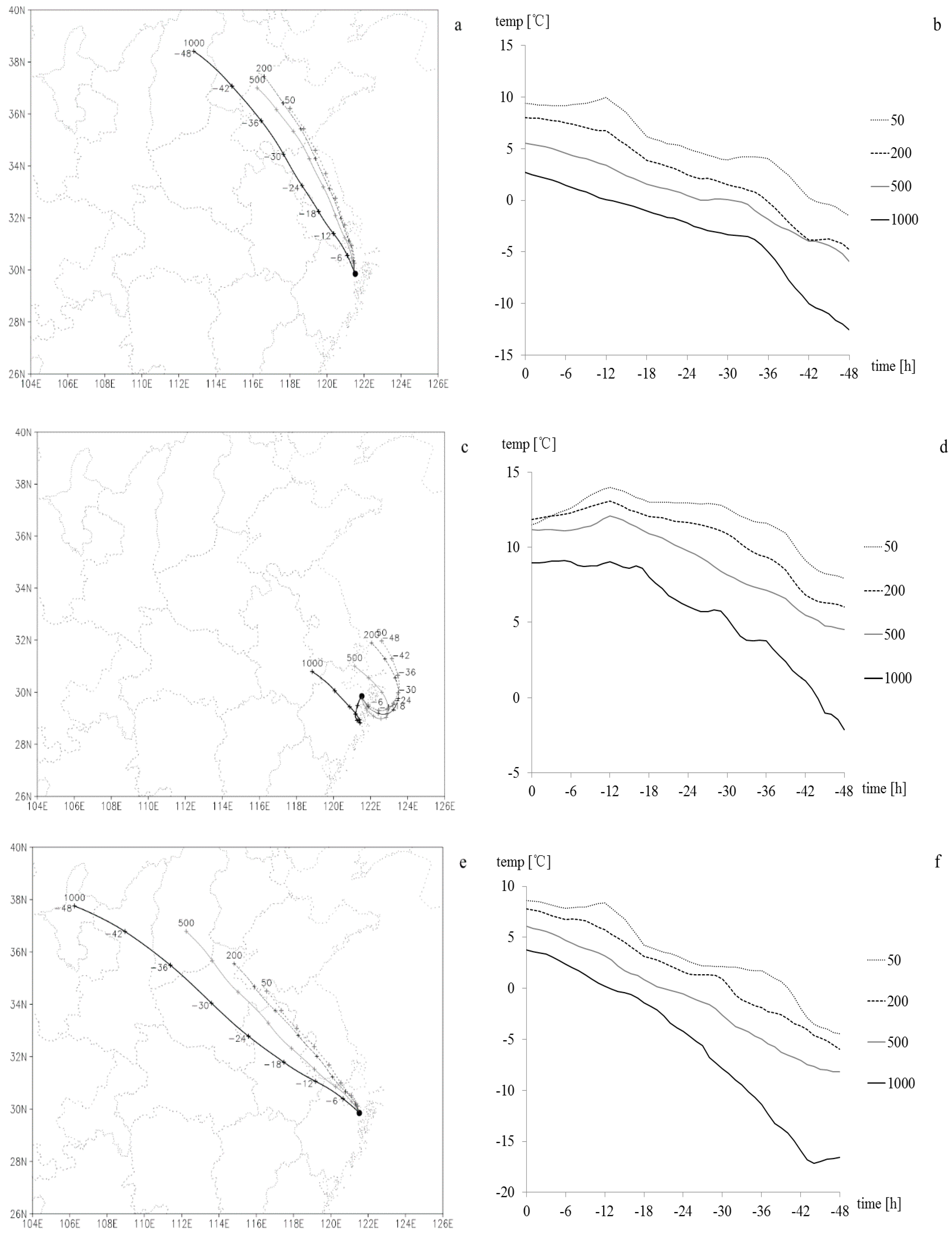
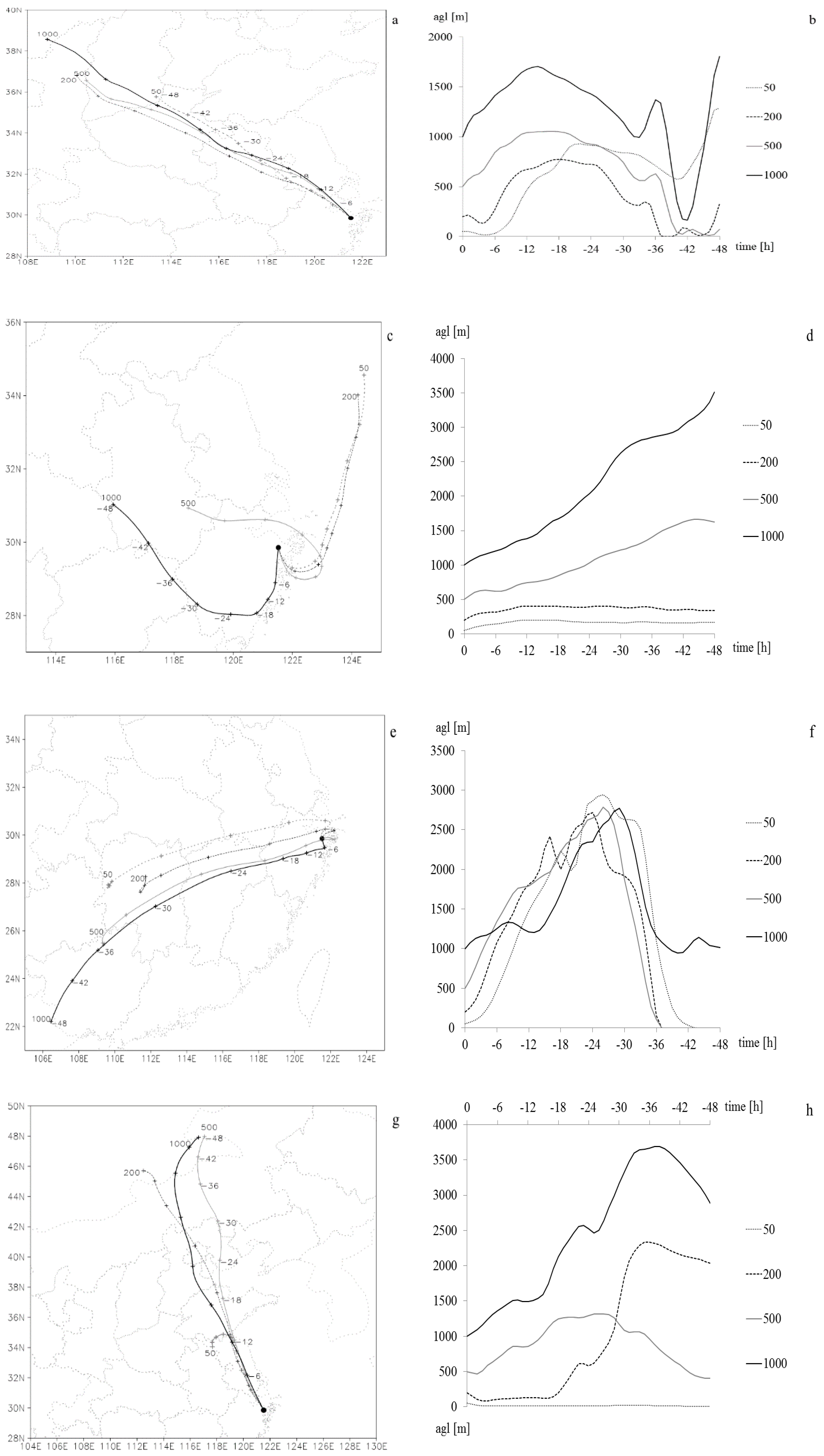
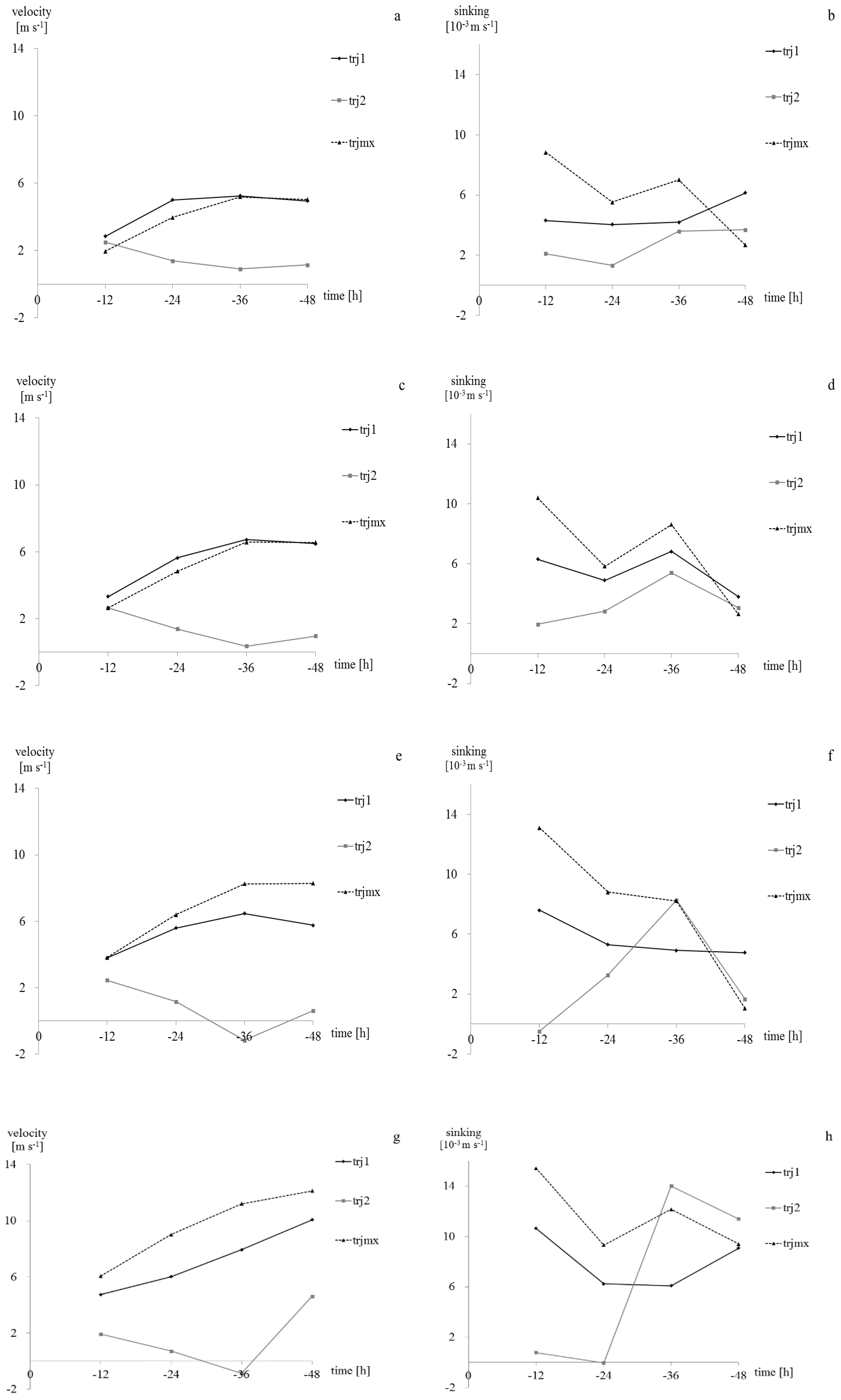
4.2. Atmospheric Stratification and Meteorological Characteristics of Pollution Types

As moderate-and-above pollution occurred only once in type 3 and never in type 4, we did not conduct trajectory element analysis on these two types.

Figure 5 illustrates the lapse rate of temperatures in four layers for pollution types 1, 2, and mx above the Environment Monitoring Center of Ningbo on moderate-and-above pollution days. The temperature of type 2 was significantly higher than those of types 1 and mx; a thermal-inversion layer appeared at 50–200 m with intensity of 0.23 °C (100 m)⁻¹; the lapse rate of temperature was only −0.22 °C (100 m)⁻¹ at 200–500 m, indicating stable middle and lower boundaries. The lapse rates of temperature for type 1 at 50–200 and 200–500 m were −0.94 °C (100 m)⁻¹ and −0.82 °C (100 m)⁻¹, respectively, both of which were very close to a dry adiabatic lapse rate, whereas the corresponding rates for type mx were −0.54 °C (100 m)⁻¹ and −0.56 °C (100 m)⁻¹, respectively. Considering that the relative humidity for types 1 and mx was approximately 50%–60% in all four layers, the logical inference is that the middle and lower boundaries were unstable and conditionally unstable for types 1 and mx respectively, but stable for type 2.

The meteorological elements in the backward trajectories varied with pollution type. Figure 6a–f illustrates the −48 to 0 h average backward trajectories at various heights (Figure 6a,c,e) and their temperature changes (Figure 6b,d,f) for pollution types 1, 2, and mx. Type 2 (Figure 6c,d) differed significantly from types 1 and mx. The −48 h aerosols at heights of 50, 200, 500, and 1000 m were approximately 256, 232, 133, and 278 km away from Ningbo, respectively. The −48 to −36 h particles slowly moved southeastward with northwesterly airflow and with a low average horizontal speed of 1.2 m s⁻¹ at 50 m. In addition, slow deposition occurred at a descending speed of 3.7 × 10⁻³ m s⁻¹. The trajectories of the −36 to 0 h particles at 50–500 m exhibited anticyclonic rotation, leading to convolution and retention of pollutants. Although both types 1 and mx particles originated from inland areas northwest of Ningbo, their source regions were distinct at different heights and distances. For trajectories at 50 m, the −48 h source region of particles of type 1 were located in Shandong, approximately 780 km northwest from Ningbo at a height of 857 m, whereas those of type mx were located at the junction of Jiangsu and Shandong, approximately 700 km from Ningbo at a height of 1089 m. For trajectories at 1000 m, the −48 h source region of particles of types 1 and mx were located in Shanxi and Ningxia at heights of 2380 and 3000 m and horizontal distances of 1240 and 1660 km, respectively. Thus, the pollutant source of type mx was higher and located further west than that of type 1 with similar trajectory layer elevation.

Regarding trajectory temperature (Figure 6b,d,f), type 2 also showed considerable differences. The −48 to −12 h temperatures of type 2 (Figure 6d) in all four layers increased gradually, indicating cold advection. By contrast, the −12 to 0 h temperatures decreased at heights of 50–500 m, indicating warm advection. The −18 to 0 h temperatures remained nearly constant at 1000 m, indicating minor temperature advection. Thus, for pollution type 2, weakening cold advection in the boundary layer during −48 to −12 h, and warm advection during −12 to 0 h in the lower boundary were observed. By contrast, for pollution types 1 and mx, the −48 to 0 h temperatures decreased in all four layers; however, the −12 to 0 h temperatures remained constant at a height of 50 m. Thus, −48 to −12 h cold advections occurred in every layer from northwest to southeast but cold air weakened at a height of 50 m from −12 to 0 h, during which the source region of particles of types 1 and mx were approximately 123 and 85 km from the start point and descended to heights of 236 and 431 m, respectively. Thus, types 1 and mx were accompanied by cold air. The −48 to 0 h particles were transported from northwest to southeast alongside cold air. From −12 to 0 h, cold air weakened in the near-surface layer, and this weakened the diffusion capacity and retention of the input particles; however, these particles continued to be transported and descended with cold air in the 200–1000 m upper boundary, which was conducive to pollutant accumulation.

Pollution types differed in terms of both horizontal and descending speeds of particles. Figure 7 illustrates these two types of speed in four layers for types 1, 2, and mx at 12 h intervals. Consistent with the results of the previous analysis, type 2 differed from the other two types. The average horizontal speed was generally <2 m s⁻¹ at each height and the −36 to −24 h speeds at heights of 500 and 1000 m were <0 m s⁻¹, implying convolution and retention of the particles that moved away from the start point. The horizontal speeds of types 1 and mx were maintained at 2–6 m s⁻¹ at 50 and 200 m and 4–12 m s⁻¹ at 500 and 1000 m, all of which were greater than those of type 2. Regarding deposition motion, the −48 to −24 h particles in all four layers for all three types descended at speeds of 3–14 × 10⁻³ m s⁻¹. Although the descending speeds did not vary much at any height, for type 2, the −24 to 0 h speeds decreased and the speeds at 500 and 1000 m were <0 m s⁻¹, indicating that the particles were no longer descending. However, types 1 and mx maintained strong deposition motion, with their −12 to 0 h descending speeds at a height of 50 m reaching a maximum at 8.8 × 10⁻³ m s⁻¹.

In summary, type 2 pollution differed significantly from types 1 and mx; its horizontal speeds were considerably slower and it even demonstrated negative speeds away from the start point, indicating convolution of the particles. Although all three pollution types were related to cold advection, the cold air in type 2 was weaker than that in types 1 and mx and was mainly limited to the upper boundary. In contrast, types 1 and mx had cold advections in all four layers that only weakened in the −12 to 0 h range at the near-surface layer. On the day before the pollution outbreak (−48 to −24 h), the particles in all three pollution types descended at almost the same speed. However for type 2, the −24 to 0 h descending speed greatly decreased and a weak ascending motion occurred in the upper and middle boundaries, whereas deposition motion in types 1 and mx became stronger. Therefore, aerosol deposition contributed less to type 2 than to types 1 and mx.

4.3. Analysis of Characteristics in Typical Cases of Different Pollution Types

Table 3. Typical cases of 4 pollution types.

Case (types)	Date (yr/m/d)	AQI	Air Pollution Level
1 (type 1)	2015/12/15	257	heavy pollution
2 (type 2)	2013/12/7	500	severe pollution
3 (type 3)	2015/12/23	251	heavy pollution
4 (type mx)	2013/12/26	312	severe pollution

lists the occurrence dates and AQI scores in typical cases of pollution types 1, 2, 3, and mx, with the highest AQI for each pollution type included.

Slight pollution had already been present for 1–3 days in Ningbo before the outbreak of each of these four cases with the primary pollutant of PM_2.5, indicating poor atmospheric diffusion capacities in these few days. Figure 8 displays the hourly PM_2.5 mass concentration evolutions of these four cases from 2 days before the outbreak (day −2 and day −1) until the occurrence day (day 0). The PM_2.5 concentrations were generally >0.1 mg m⁻³ and did not vary with traffic peaks or valleys, with the AQI reaching the slight pollution level or above. The PM_2.5 concentrations of cases 1, 3, and 4 began steadily increasing from 18:00 h on day −1, whereas the increase in case 2 began from 16:00 h on day −2. This observation indicates that levels of aerosols (including PM₁₀ and PM_2.5) were high during slight pollution episodes on days −2 and −1 with poor atmospheric diffusion capacities. The superposition of aerosol particles ultimately led to heavy-and-above (including heavy and severe) pollution. Therefore, a typical pollution case did not result from one round of pollutant transport but rather from the final result of continuous superposition of multiple rounds of pollutant transport.

Figure 9 illustrates the −48 h backward trajectories (Figure 9a,c,e,g) and their height changes (Figure 9b,d,f,h) in various layers of the four cases. The heights of pollutant sources and trajectories differed. For case 1, the backward trajectories on day −1 to day 0 were identical in some layers (Figure 9a,b). The −48 h pollutant sources in all layers were located in the northwest inland region 1000–1500 km away from Ningbo. The average 12 h horizontal speed in each layer remained nearly constant at 5–10 m s⁻¹. The −42 to −12 h particles in each layer were elevated with a maximum speed of 13 × 10⁻³ m s⁻¹; thereafter, the −24 to 0 h particles in the boundary layer descended at an average speed of 6 × 10⁻³ m s⁻¹, resulting in a continuous increase in PM_2.5 concentration on day 0 (Figure 8).

Case 2 was different (Figure 9c,d). The −48 to 0 h trajectories at 200 and 50 m did not descend, and the deposition of the −12 to 0 h trajectories at 500 and 1000 m was not obvious. The −24 h pollutant sources in each layer were within 300 km of Ningbo. Therefore, the increases in pollutant concentrations in the lower boundary from −24 to 0 h were due to the circulation of vicinal particles, whereas deposition had little effect on the severe pollution outbreak.

Case 3 was the only heavy pollution outbreak belonging to type 3, which was a low-probability event. Trajectory analysis revealed that the particles originated from the southwest of Ningbo (Figure 9e). At −48 h, the particles at 50–500 and 1000 m were 950–1300 and 1730 km from the start point, respectively. The particles were elevated from −48 to −30 h and then descended from −24 to 0 h (Figure 9f). At −12 h, the particles in each layer were less than 100 km from Ningbo. Thereafter, when approaching Ningbo, the particles at heights of 50 and 200 m turned from north to south alongside weak cold air, whereas at heights of 500 and 1000 m, they moved from south to north. The particles in each layer descended and met in Ningbo, resulting in a steady increase in particle concentration on day 0 for case 3. Hence, the input particles 1000 km away from the southwest of Ningbo were transported northeastward by southwesterly airflows and elevated to middle and lower troposphere layers below 3000 m because of the uplifting effect; they then descended from −24 to 0 h. When they were 100 km away from Ningbo, the low-level particles turned from north to south, whereas the middle-upper-layer particles moved from south to north, resulting in their deposition in Ningbo. In addition, the slight-and-above pollution on day −2 to day −1 implied poor air diffusion capacities. Ultimately input particles and poor diffusion capacities led to the only heavy pollution case that occurred in southwesterly airflow.

Case 4 was the most typical case of type mx; it was largely the same as case 1 but differed in some aspects. Although both cases originated in the northwest of Ningbo, they differed in terms of pollutant sources, particle elevation, and deposition height. For case 4, the −48 h particles at a height of ≥200 m were >1900 km from Ningbo (Figure 9g), which was farther than the distance in case 1, and those at a height of 50 m were <600 km from Ningbo, which was closer than the distance in case 1. During southeastward transport, the −48 to −30 h particles first were elevated and then gradually descended, except for those at a height of 50 m in case 4 (Figure 9h). The impact of deposition on the pollution outbreak mainly occurred at heights of ≥200 m. Therefore, alongside long-range particle transport, deposition in the middle and lower troposphere layers, a backdrop of continuous pollution, and horizontal input of vicinal pollutants in the near-surface layer finally led to the severe pollution outbreak in case 4.

The aforementioned analysis results for the four typical pollution cases indicated that continuous slight-and-above pollution on day −2 to day −1 represented not only high pollutant concentrations but also poor atmospheric diffusion capacities; the input particles on the pollution outbreak day most likely originated from the northwest of Ningbo. However, when the circulation conditions were suitable, these particles may have originated from a southwesterly or easterly direction. In addition, the horizontal distance from the source region to Ningbo greatly varied according to direction. The particles in the upper boundary layer at heights of 500 and 1000 m descended but the input particles in the lower-boundary layer at heights of 50 and 200 m did not necessarily descend. Thus, focusing on the lower-boundary pollution situation of upstream areas can provide a significant reference for local pollution forecasting.

5. Conclusions

Taking Ningbo as the representative city of coastal Zhebei, based on observation data from the Environment Monitoring Center of Ningbo, hourly meteorological observation data from Zhejiang AWS, and US NCEP-GDAS data, air quality characteristics in Ningbo were statistically analyzed, and the HYSPLIT model was used to conduct backward trajectory clustering analysis and trajectory feature statistical analysis. The results are described as follows.

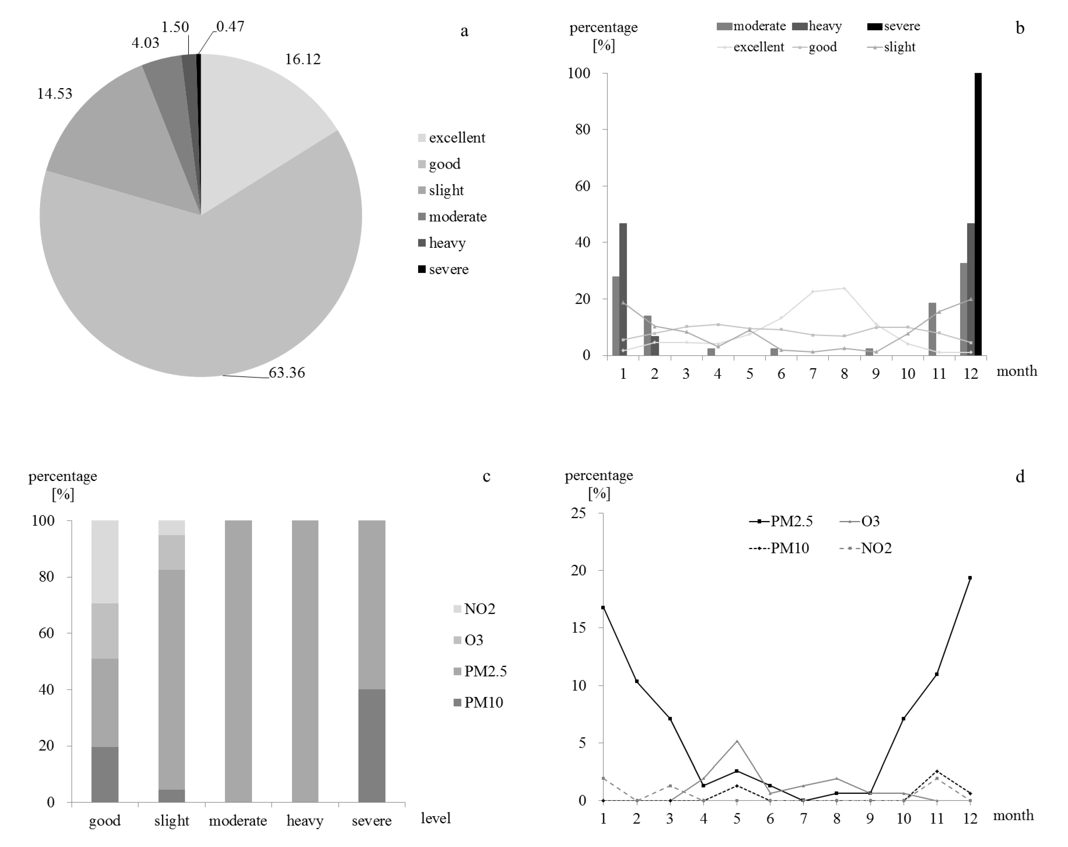
• The percentage of excellent and good air quality in Ningbo was approximately 80% and that of moderate-and-above pollution was approximately 6%. The monthly variation in the percentage of slight-and-above pollution was U shaped; the higher the pollution level, the wider was the lower half of the U-shaped curve. Most moderate-and-above pollution occurred from November to February and the primary pollutant was PM_2.5. Haze of visibility <5000 m was common in Zhebei during moderate-and-above pollution days.
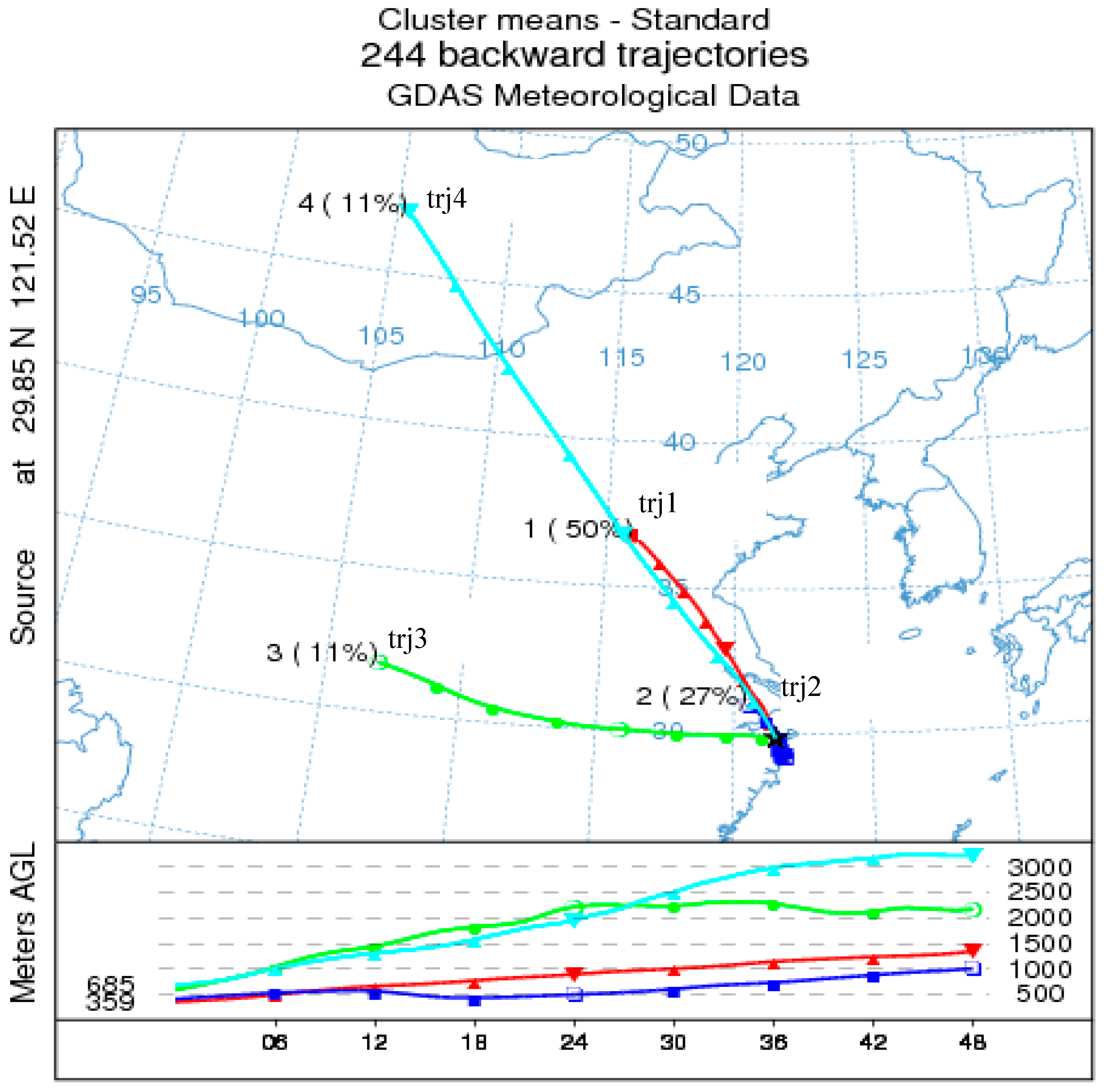
• For moderate-and-above pollution in Ningbo, 77% of the pollutants originated from vicinal areas within 1000 km to the northwest; of these, nearly 27% were related to close-range pollution within 200 km. The average height of −48 h pollutant sources did not exceed 1500 m; these sources mainly affected the air quality of the lower boundary. Approximately 22% originated from remote areas farther than 1400 m with long-range transport and deposition in the middle and lower troposphere above 2500 m; these sources mainly affected the air quality of the middle and upper boundaries above 600 m.
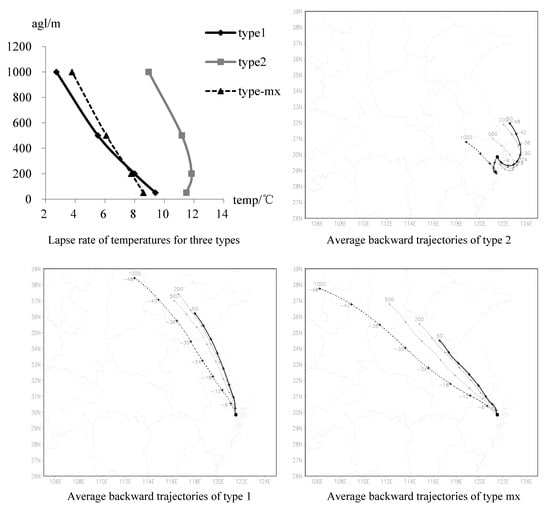
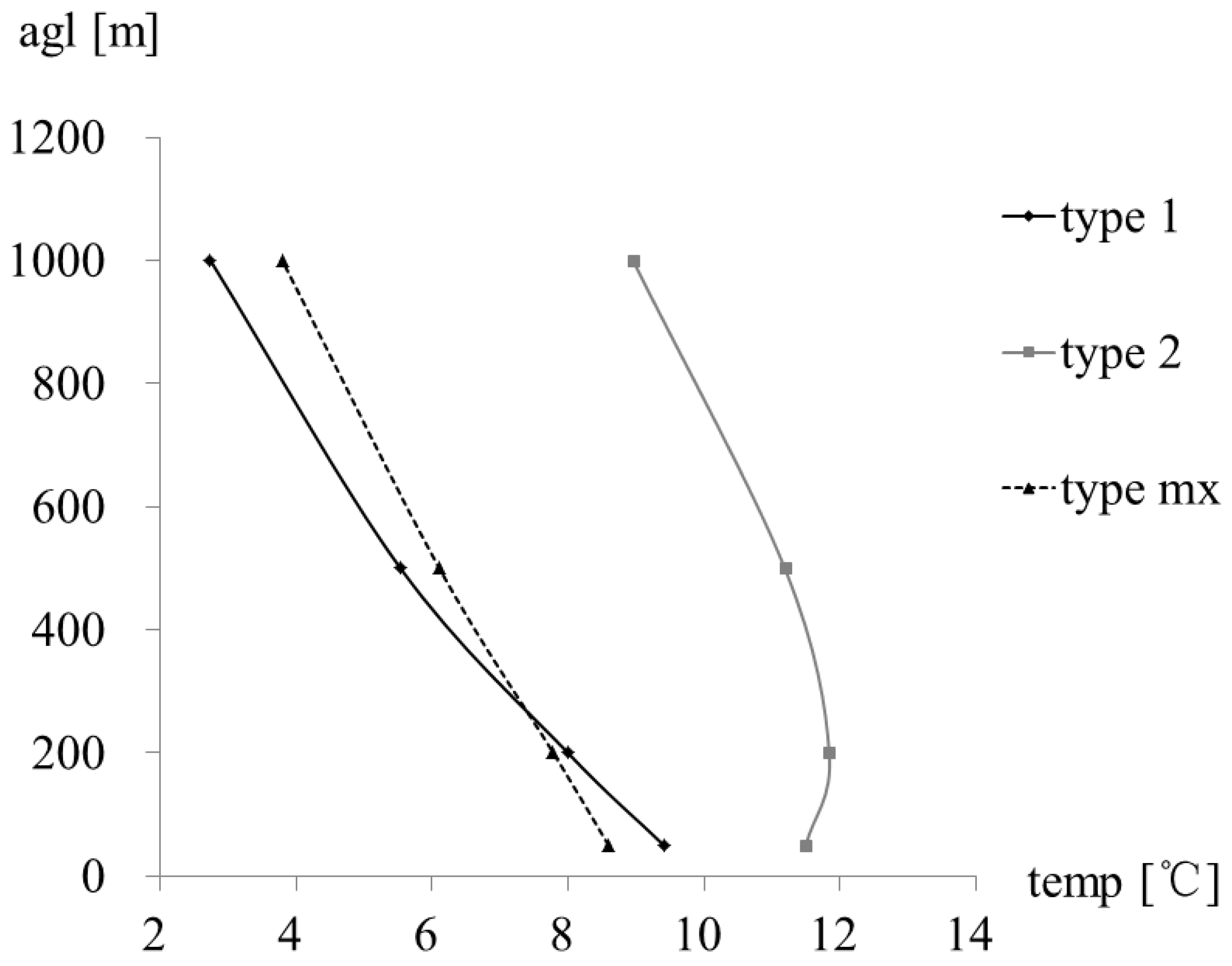
• Moderate-and-above pollution was mainly a result of three trajectory types: mx, 1, and 2. Type 2 differed significantly from the other two types because atmospheric stratification in the middle- and lower-boundary layers was stable. By contrast, types 1 and mx respectively occurred in the unstable and conditionally unstable layers. Furthermore, type 2 differed significantly from types 1 and mx in terms of meteorological elements, namely the temperature, horizontal speed, and descending speed in each layer.
• The characteristic analysis of typical cases of various pollution types revealed that the pollution outbreak did not result from one round of pollutant transport but rather was the final result of continuous superposition of multiple rounds of pollutant transport. The input particles on the pollution outbreak day most likely originated northwest of Ningbo but under suitable circulations may have originated from a southwesterly or easterly direction.

References

1. Li, X.F.; Zhang, M.J.; Wang, S.J.; Zhao, A.F.; Ma, Q. Variation characteristics and influencing factors of air pollution index in China. Environ. Sci. 2012, 33, 1936–1943. (In Chinese) [Google Scholar]
2. Zhang, X.Y.; Sun, J.Y.; Wang, Y.Q.; Li, W.J.; Zhang, Q.; Wang, W.Q.; Quan, J.N.; Cao, G.L.; Wang, J.Z.; Yang, Y.Q.; et al. Factors contributing to haze and fog in China. Chin. Sci. Bull. 2013, 58, 1178–1187. (In Chinese) [Google Scholar] [CrossRef]
3. Charlson, R.J.; Schwartz, S.E.; Hales, J.M.; Cess, R.D.; Coakley, J.A.; Hansen, J.E.; Hofmann, D.J. Climate forcing by anthropogenic aerosols. Science 1992, 255, 423–430. [Google Scholar] [CrossRef] [PubMed]
4. Ramanathan, V.; Crutzen, P.J.; Kiehl, J.T.; Rosenfeld, D. Aerosols, climate, and the hydrological Cycle. Science 2001, 294, 2119–2124. [Google Scholar] [CrossRef] [PubMed]
5. Lohmann, U.; Feichter, J. Global indirect aerosol effects: A review. Atmos. Chem. Phys. 2005, 5, 715–737. [Google Scholar]
6. Kosmopoulos, P.G.; Kaskaoutis, D.G.; Nastos, P.T.; Kambezidis, H.D. Seasonal variation of columnar aerosol optical properties over Athens, Greece, based on modis data. Remote Sens. Environ. 2008, 112, 2354–2366. [Google Scholar] [CrossRef]
7. Li, Z.Q.; Gu, X.; Wang, L.; Li, D.H.; Li, K.T.; Dubovik, O.; Schuster, G.; Goloub, P.; Zhang, Y.; Li, L.; et al. Aerosol physical and chemical properties retrieved from ground-based remote sensing measurements during heavy haze days in Beijing winter. Atmos. Chem. Phys. 2013, 13, 10171–10183. [Google Scholar] [CrossRef] [Green Version]
8. Solmon, F.; Nair, V.S.; Mallet, M. Increasing Arabian dust activity and the Indian summer monsoon. Atmos. Chem. Phys. 2015, 15, 8051–8064. [Google Scholar] [CrossRef] [Green Version]
9. Muhammad, F.K.; Naila, Y.; Farrukh, C.; Imran, S. Temporal variability and characterization of aerosols across the Pakistan region during the winter fog periods. Atmosphere 2016, 7, 67. [Google Scholar]
10. Sampson, P.D.; Richards, M.; Szpiro, A.A.; Bergen, S.; Sheppard, L.; Larson, T.V.; Kaufman, J.D. A regionalized national universal kriging model using partial least squares regression for estimating annual PM2.5 concentrations in epidemiology. Atmos. Environ. 2013, 175, 383–392. [Google Scholar]
11. Salameh, D.; Detounay, A.; Pey, J.; Pérez, N.; Liguori, F.; Saraga, D.; Bove, M.C.; Brotto, P.; Cassola, F.; Massabò, D.; et al. PM2.5 chemical composition in five European Mediterranean cities: A 1-year study. Atmos. Res. 2015, 155, 102–117. [Google Scholar] [CrossRef]
12. Eeftens, M.; Tsai, M.Y.; Ampe, C.; Anwander, B.; Beelen, R.; Bellander, T.; Cesaroni, G.; Cirach, M.; Cyrys, J.; Hoogh, K.D.; et al. Spatial variation of PM2.5, PM10, PM2.5 absorbance and PM coarse concentrations between and within 20 European study areas and the relationship with NO2—Results of the ESCAPE project. Atmos. Environ. 2012, 62, 303–317. [Google Scholar] [CrossRef]
13. European Union. Air Quality in Europe—2016 Report; European Environment Agency EEA Report No. 28/2016; Publications Office of the European Union: Luxembourg, 2016. [Google Scholar]
14. Draxler, R.R.; Hess, G.D. An overview of the HYSPLIT_4 modeling system for trajectories dispersion and deposition. Aust. Meteorol. Mag. 1998, 47, 295–308. [Google Scholar]
15. Escudero, M.; Stein, A.F.; Draxler, R.R.; Querol, X.; Alastuey, A.; Castillo, S.; Avila, A. Source apportionment for African dust outbreak over the Western Mediterranean using the HYSPLIT model. Atmos. Res. 2011, 99, 518–527. [Google Scholar] [CrossRef]
16. Chen, B.; Stein, A.F.; Maldonado, P.G.; Campa, A.M.; Castanedo, Y.G.; Castell, N.; Rosa, J.D. Size distribution and concentrations of heavy metals in atmospheric aerosols originating from industrial emissions as predicted by the HYSPLIT model. Atmos. Environ. 2013, 71, 234–244. [Google Scholar]
17. Cheng, S.Y.; Wang, F.; Li, J.B.; Chen, D.S.; Li, M.J.; Zhou, Y.; Ren, Z.H. Application of trajectory clustering and source apportionment methods for investigating trans-boundary atmospheric PM10 pollution. Aerosol. Air Qual. Res. 2013, 13, 333–342. [Google Scholar]
18. Wang, H.; Xue, M.; Zhang, X.Y.; Liu, H.L.; Zhou, C.H.; Tan, S.C.; Che, H.Z.; Chen, B.; Li, T. Mesoscale modeling study of the interactions between aerosols and PBL meteorology during a haze episode in Jing–Jin–Ji (China) and its nearby surrounding region—Part 1: Aerosol distributions and meteorological features. Atmos. Chem. Phys. 2015, 15, 3257–3275. [Google Scholar]
19. Tatsuta, S.; Shimada, K.; Chan, C.K.; Kim, Y.P.; Lin, N.H.; Takami, A.; Hatakeyama, S. Contributions of long-range transported and locally emitted nitrate in size-segregated aerosols in Japan at Kyushu and Okinawa. Aerosol. Air Qual. Res. 2017, 17, 3119–3127. [Google Scholar] [CrossRef]
20. Stein, A.F.; Draxler, R.R.; Rolph, G.D.; Stunder, B.J.B.; Cohen, M.D.; Ngan, F. Noaa’s HYSPLIT atmospheric transport and dispersion modeling system. Bull. Am. Meteorol. Soc. 2015, 96, 2059–2077. [Google Scholar] [CrossRef]
21. Zhang, Y.; Liu, Z.H.; Lv, X.T.; Zhang, Y.; Qian, J. Characteristics of the transport of a typical pollution event in the Chengdu area based on remote sensing data and numerical simulations. Atmosphere 2016, 7, 127. [Google Scholar] [CrossRef]
22. Zheng, Y.; Che, H.Z.; Zhao, T.L.; Xia, X.G.; Gui, K.; An, L.C.; Qi, B.; Wang, H.; Wang, Y.Q.; Yu, J.; et al. Aerosol optical properties over Beijing during the World Athletics Championships and Victory Day Military Parade in August and September 2015. Atmosphere 2016, 7, 47. [Google Scholar]
23. Yang, W.L.; Wang, G.C.; Bi, C.J. Analysis of long-range transport effects on PM2.5 during a short severe haze in Beijing, China. Aerosol. Air Qual. Res. 2017, 17, 1610–1622. [Google Scholar] [CrossRef]
24. Yao, R.S.; Tu, X.P.; Zhang, X.W.; Xu, D.F.; Yang, D.; Gu, X.L. Analysis on a rare persistent heavy pollution event in Ningbo. Acta Meteorol. Sin. 2017, 2, 342–355. [Google Scholar]
25. Wu, D.; Zhang, F.; Ge, X.L.; Yang, M.; Xia, J.R.; Liu, G.; Li, F.Y. Chemical and light extinction characteristics of atmospheric aerosols in suburban Nanjing, China. Atmosphere 2017, 8, 149. [Google Scholar] [CrossRef]
26. Liu, D.Y.; Liu, X.J.; Wang, H.B.; Li, Y.; Kang, Z.M.; Cao, L.; Yu, X.N.; Chen, H. A New type of haze? The December 2015 purple (magenta) haze event in Nanjing, China. Atmosphere 2017, 8, 76. [Google Scholar] [CrossRef]
27. Lu, X.; Mao, F.Y.; Pan, Z.X.; Gong, W.; Wang, W.; Tian, L.Q.; Fang, S.H. Three-dimensional physical and optical characteristics of aerosols over central China from long-term CALIPSO and HYSPLIT Data. Remote Sens. 2018, 10, 314. [Google Scholar]
28. Yu, Z.Y.; Li, Z.Q.; Gao, D.W.; Wang, K. Feature analysis of air quality and atmospheric self-purification capability in Zhejiang. Meteorol. Mon. 2017, 43, 323–332. (In Chinese) [Google Scholar]
29. The Ministry of Environmental Protection of the People’s Republic of China. GB 3095-2012 Ambient Air Quality Standard; HJ633-2012 Technical Regulation on Ambient Air Quality Index; The Ministry of Environmental Protection of the People’s Republic of China: Beijing, China, 2012.
Figure 1. The percentages of air quality levels in Ningbo (a), the percentage variation of each air quality level by month (b), the composition of primary pollutants of each level (c), the fractions of primary pollutants by month for slight pollution (d), from 1 June 2013 to 31 May 2016.
Atmosphere 10 00120 g001
Figure 2. The average distribution of automatic visibility in Zhejiang for 64 moderate-and-above pollution episodes (unit: m, the cross location marked “NB” is the city Ningbo).
Atmosphere 10 00120 g002
Figure 3. The average hourly individual air quality index (IAQI) evolutions of six major pollutants for moderate-and-above pollution from 2 days before the outbreak (day −2 and −1) until the occurrence day (day 0) in Ningbo.
Atmosphere 10 00120 g003
Figure 4. The −48 h average backward trajectories for moderate-and-above pollution episodes in Ningbo.
Atmosphere 10 00120 g004
Figure 5. The lapse rate of temperatures at four layers for 3 types above the Environment Monitoring Center of Ningbo on moderate-and-above pollution days.
Atmosphere 10 00120 g005
Figure 6. Moderate-and-above pollution events average backward trajectories from −48 h and their temperature changes at various heights for in autumn and winter from 2013 to 2016 (a,b: type 1; c,d: type 2; e,f: type mx).
Atmosphere 10 00120 g006
Figure 7. The average horizontal speeds (a: 50 m, c: 200 m, e: 500 m, g: 1000 m) and descending speeds (b: 50 m, d: 200 m, f: 500 m, h: 1000 m) in four layers at 12 h time intervals.
Atmosphere 10 00120 g007
Figure 8. The hourly PM2.5 mass concentration evolutions of the four typical cases.
Atmosphere 10 00120 g008
Figure 9. The −48 h backward trajectories (a,c,e,g) and their height change (b,d,f,h) in various layers of the four typical cases.
Atmosphere 10 00120 g009