Article

Comparison of Columnar, Surface, and UAS Profiles of Absorbing Aerosol Optical Depth and Single-Scattering Albedo in South-East Poland

by
Michał T. Chiliński
1,*,
Krzysztof M. Markowicz
1,
Olga Zawadzka
1,
Iwona S. Stachlewska
1,
Justyna Lisok
1 and
Przemysław Makuch
2
1
Institute of Geophysics, Faculty of Physics, University of Warsaw, 02-093 Warszawa, Poland
2
Institute of Oceanology, Polish Academy of Sciences, 81-712 Sopot, Poland
*
Author to whom correspondence should be addressed.
Atmosphere 2019, 10(8), 446; https://doi.org/10.3390/atmos10080446
Submission received: 3 July 2019 / Revised: 23 July 2019 / Accepted: 23 July 2019 / Published: 2 August 2019
(This article belongs to the Special Issue Remote Sensing of Aerosols)

Abstract

:
The impact of absorbing aerosols on climate is complex, with their potential positive or negative forcing, depending on many factors, including their height distribution and reflective properties of the underlying background. Measurement data is very limited, due to insufficient remote sensing methods dedicated to the retrieval of their vertical distribution. Columnar values of absorbing aerosol optical depth (AAOD) and single scattering albedo (SSA) are retrieved by the Aerosol Robotic Network (AERONET). However, the number of available results is low due to sky condition and aerosol optical depth (AOD) limitation. Presented research describes results of field campaigns in Strzyżów (South-East Poland, Eastern Europe) dedicated to the comparison of the absorption coefficient and SSA measurements performed with on-ground in-situ devices (aethalomter, nephelometer), small unmanned aerial system (UAS) carrying micro-aethalometer, as well as with lidar/ceilometer. An important aspect is the comparison of measurement results with those delivered by AERONET. Correlation of absorption to scattering coefficients measured on ground (0.79) and correlation of extinction on ground to AOD measured by AERONET (0.77) was visibly higher than correlation between AOD and AAOD retrieved by AERONET (0.56). Columnar SSA was weakly correlated with ground SSA (higher values of columnar SSA), which were mainly explained by hygroscopic effects, increasing scattering coefficient in ambient (wet conditions), and partly high uncertainty of SSA retrieval. AAOD derived with the use of profiles from UAS up to PBL height, was estimated to contribute in average to 37% of the total AAOD. A method of AAOD estimation, in the whole troposphere, with use of measured vertical profiles of absorption coefficient and extinction coefficient profiles from lidars was proposed. AAOD measured with this method has poor correlation with AERONET data, however for some measurements, within PBL, AAOD was higher than reported by AERONET, suggesting potential underestimation in photometric measurement under particular conditions. Correlation of absorption coefficient in profile to on ground measurements decrease with altitude. Measurements of SSA from drones agree well with ground measurements and are lower than results from AERONET, which suggests a larger contribution of absorbing aerosols. As an alternative for AAOD estimation in case of lack of AERONET AAOD data simple models are proposed, which base on AOD scaling with SSA measured with different methods. Proposed solution increase potential of absorption coefficient measurements in vertical profiles and columns of the atmosphere. Presented solutions make measurements of absorption coefficients in vertical profiles more affordable and allow rough estimation of columnar values for the whole atmosphere.

1. Introduction

The climate impact of absorbing aerosols, such as organic and black carbon (BC) particles originating from fossil fuel combustion or biomass burning, mineral dust and volcanic ash, is still poorly known [1]. It is due to several reasons, mainly too few observations of absorbing aerosol, large uncertainties in direct measurements and too simplified description of physical processes involving absorbing aerosols used for climate modelling [1,2]. Along with the greenhouse gases, the absorbing aerosols are considered to be very important contributors to the global warming, as they are a crucial component for the energy balance in the climate system [3,4,5,6]. In the case of absorbing aerosol not only amount of absorbing particles but also vertical profiles are important for climate processes [5,7]. The simulations performed by climate models, which include only an idealised absorbing aerosol scheme, show that the average surface temperature is a function of the altitude at which the layer of the absorbing particles exists [6]. For example, increase of altitude of absorbing particles decreases the surface temperature and reduces the rainfall [8]. Koch and Del Genio [2] report that the aerosol climate impact depends on the aerosol location with respect to, and in relation to clouds. Taking into account that optical properties of absorbing particles could vary along the vertical profile, it could significantly influence the assessment of the direct aerosol effect [9,10,11].
For absorbing aerosols of desert dust, taking into account their actual vertical profile instead of the climatic value of their optical properties, leads to change in the radiative forcing calculation of about a 100% [9].
The amount of absorbing particles in the atmosphere can be defined by the absorbing aerosol optical depth (AAOD) and by single-scattering albedo (the ratio of absorbed to attenuated incident sunlight, SSA). Such parameters are key data products of the ground-based Aerosol Robotic Network (AERONET) [12]. Retrieval of AAOD and SSA is limited to completely clear-sky conditions. Dubovik [13] reports that all absorption-related products are strongly uncertain when AOD is low. For the SSA retrieved from AERONET observations the uncertainty (95% confidence) is ±0.03 for AOD (440 nm) above 0.4 and ±0.06 for lower AOD values [13]. AERONET recommendation for using absorption data (Level 2.0) is defined by a AOD (440 nm) threshold of 0.4. Unfortunately, this limitation greatly reduces spatial and temporal coverage of SSA and AAOD. Andrews [14] reports, based on AeroCom Phase II models, that 95% of global AOD and 89% over land AOD (440 nm) values are below 0.4. Consequently, AERONET Level 2.0 absorption-related data represents a small number of observation and is biased towards moderate to high aerosol loadings. In some regions (e.g., Arctic) AOD at 440 nm above the 0.4 is measured rarely, therefore AERONET information on SSA and AAOD are usually not available there. In several studies the data from AERONET Level 1.5 are used. Andrews [14] and Schafer [15] utilized the Level 1.5 SSA and AAOD in the cases when there was a corresponding valid Level 2.0 of AOD, however in such cases the absorption in the atmospheric column could be significantly overestimated in comparison with the in-situ observation. Andrews [14] suggested that observed discrepancy in SSA cannot definitively be attributed to either technique, as in-situ measurements have also significant uncertainties. In-situ observations of aerosol absorption are mostly based on filter systems, such as aethalometers, providing a relatively simple but indirect method of measuring optical particle absorption. However, two well-know artefacts affect these absorption measurements. The first effect, called a filter-loading effect, reduces the optical path length due to shadowing. The second effect is related to multiple scattering between aerosol and filter fibres [16]. For accurate estimation of aerosol coefficients a number of corrections must be applied (e.g., [17,18,19,20]. Aerosol absorption coefficient can be also measured based on photoacoustic techniques. In this case the scattering effects are negligible and the signal measured by a sensitive microphone is a direct function of aerosol absorption [21]. Unfortunately this kind of measurements is not common yet. In addition, photoacoustic method is not efficient for very clean condition, due to high noise of the instrument [22].
The absorption coefficient and SSA measurements at the ground level are not sufficient to validate the AERONET retrievals products, being defined in the atmospheric vertical column. Representation of surface aerosol absorption and surface SSA for whole column is not well known, in contrary to the case of the surface aerosol scattering and surface AOD relationship, which is used to transform the satellite AOD observation to particulate matter (PM) concentration at the ground level. This is justifying the need of vertical profiles of aerosol absorption. In-situ measurements via airborne measurements are expensive and therefore UAS and tethered balloons are used more frequently for this purpose. Ferrero [23] and Markowicz [22] report absorption profiles measured by micro-aethalometer mounted on tethered balloons up to 1–2 km above ground level (a.g.l.) in the Arctic. Profiles of absorption coefficient as well as BC concentration measured from UAS were obtained in different regions by numerous researchers [24,25,26,27]. Such measurements are usually limited to the lower troposphere, and therefore an estimation of the AAOD in whole atmospheric column is uncertain when the significant part of aerosol is present above the limit of the instrument ascent. Active remote sensing, such as complex Raman lidars, are natural candidates for vertical profiles of absorption measurements. However, known inversion methods that require lidar derived aerosol backscattering and extinction coefficients, struggle to derive SSA profiles with low uncertainty demanded by models [28,29,30,31,32]. Lidars do not provide directly profiles of aerosol absorbing coefficient for calculation of SSA. Therefore uncertainty of lidar-derived SSA is high, as a result of uncertainties introduced by the inversion procedure itself and uncertainties of optical input parameters i.e., backscattering and extinction coefficients. Combination of lidar profiling and sunphotometer measurements were proposed an improvement for the sole measurements with lidars [33]. Methods that combine lidar remote sensing with in-situ sounding of atmosphere are one of solutions to this problem. Markowicz [22] developed a method for the estimation of vertical profiles of SSA based on Raman lidar and micro-aethalometer tethered balloon soundings in the Arctic. The main limitation of their method is related to significant noise of the absorption coefficient measured in the clean conditions when the vertical speed of balloon is above 1–2 m/s. Uncertainties estimated for SSA vary between ±0.01 and ±0.04.
In this paper, an easy to replicate, low-cost, and fast in terms of temporal-resolution (a few dozen of minutes) method for retrieval of vertical variability of aerosol absorption coefficient, SSA and AAOD is proposed, tested and elaborated. The method is based on a combination of in-situ profiles acquired by an aethalometer and a radiosonde on a UAS [26] with a simple aerosol scattering lidar/ceilometer or Raman lidar profiles, supported by columnar parameters sensed by photometer and surface in-situ measurements by aethalometer and nephelometer. The main goal of this study is a comparison of the absorption information measured at ground level with the absorption vertical profile, as well as absorption defined in the whole atmospheric column for a background station in South-East Poland. Focus of this work was set on determination how in-situ observations of absorption coefficient on ground and in the low troposphere could be used for reasoning about the whole atmospheric column, as well as comparison of estimation based on those measurements with AERONET Level 1.5 products obtained during clean conditions.
The paper is structured as follows. Section 2 includes description of the instrumentation and measurement setup. The next Section 3 is dedicated to methods of aerosol absorption coefficient and SSA retrievals (extinction coefficient measurements from lidar), including discussion of aethalometer calibration. Results are presented in Section 4, divided into subsections dedicated to columnar and ground measurements, vertical profiling and simple modelling of AAOD based on other measurements. Work is summarized in Section 5, where major finding are concluded.

2. Instrumentation

Several field experiments were conducted for verification of the proposed profiling method. During those experiments different sets of sensors were used. The location of measurements was Poland AOD observational site, SolarAOT, in Strzyżów (49.8786 N, 21.8613 E, south-eastern Poland, 464 m ASL, Figure 1, with the main campaign in summer 2015 (June–August).
The typical measurement configuration comprised of: (1) the UAS (Versadones VersaX6-sci) equipped with the AethLabs AE-51 and the radiosonde Vaisala RS92-SGP, (2) on ground in-situ instruments: the aethalometer McGee AE-31 and the nephelometer Ecotech Aurora 4000, (3) ground based remote-sensors: the near-range receiver, near-range aerosol Raman lidar (NARLa), of the PollyXT Raman lidar, the Raymetrics LB-10 lidar, the Ceilometer JenOptik CHM-15k, and the AERONET Cimel-318 sunphotometer. For profiling purpose, over 100 UAS flights were conducted, from which 78 was with fully functional payload for black carbon concentration and absorption coefficient profiling. Profiles were collected regardless of time of a day, when meteorological conditions were acceptable for safe UAS operations. Data was mainly acquired during three weekly intensive operation periods in June (11 profiles), July (26 profiles), and August (41 profiles) 2015. Mean height of measured profile was 960 m above ground level (median of 1005 m a.g.l.). In the following subsections, a short description of the instruments is given.

2.1. In-Situ

2.1.1. Aethalometer AE-51

The micro-aethalometer AE-51 is a portable device of AethLabs to measure the equivalent black carbon (eBC) concentration as well as absorbing coefficient. The infrared radiation (880 nm) is used to measure transmission through a Teflon-coated fiber glass filter. A change in filter attenuation is then translated to the eBC. Aethalometer with internal data logger and battery is enclosed in a housing with dimensions of 117 mm × 66 mm × 38 mm and weights about 280 grams. The device can be operated on batteries over 24 h. Filter supplied by the manufacturer is made of T60 Teflon-coated borosilicate fibreglass filter material. Filters are exchanged manually (single-slot in the device housing), depending on the amount of eBC concentration, to maintain dimensionless attenuation (ATN) below 20. In this study AE-51 was configured with one second resolution, which corresponds to 3–4 m vertical resolution. The eBC measurement precision declared by the manufacturer is of ±0.1 μ g/m 3 for 60 second averaging. Ferrero [23] investigated the accuracy of the eBC measurement by AE-51 and found that 20 ng/m 3 can be considered the limit above which the single measurement is not affected by instrumental noise. The instrument was calibrated for the air flow of 0.2 L/min by the TetraCal (BGI Instruments) volumetric air flow calibrator, before every flight session. The flight data was synchronized with other equipment by setting the internal clock with network time protocol. Data processing for these instruments is described in the Section 3.1.

2.1.2. Aethalometer AE-31

Spectral absorption coefficient was derived from the aethalometer AE-31, designed for real-time continuous measurements of eBC [34]. This aethalometer, similarly to AE-51, continuously draws air samples through the inlet port, depositing the aerosols on a fibrous quartz filter media (Pallflex, type Q250F), while performing continuous optical measurements of that filter media. Filter change can be set automatically at an ATN value limit set by the operator. Two detectors monitor the light transmission through the filter; one measures the light beam attenuation through the sample and filter and the other measures the light passing through a clean, reference filter section. The aethalometer measures the transmission through the filter over the wide spectrum of wavelengths (in this study 370, 470, 520, 590, 660, 880, 950 nm), computes and reports the eBC [ng/m 3 ] for given apparent mass attenuation cross sections σ A T N as in formula Equation (1).
e B C = d A T N d t A Q · σ A T N ,
where A is a sample spot area and Q is the volumetric flow rate. During the experiment, the flow speed was set 4 L/min, while averaging time of 5 min. The flow rate was calibrated by the TetraCal (BGI Instruments) volumetric air flow calibrator. Inlet to AE-31 was mounted about 3 m a.g.l. It is known that all filter-based instruments suffer from several artefacts [18,20,35]. Therefore, compensation to the data was applied to determine the spectral absorption coefficients. This method is discussed in detail in Section 3.1.

2.1.3. Nephelometer Aurora 4000

The surface aerosol scattering properties were measured by a three-wavelength Aurora 4000 polar nephelometer (Aurora 4000, Etotech). This nephelometer was based on an array of several LEDs (light emitting diodes) opal glass light source [36]. The advantage of LED light sources is that they generate a fraction of the heat generated by halogen flash lamps in traditional nephelometer. The Aurora 4000 implements a hemispheric backscatter mode: a motor driver backscatter shutter, which is attached to the light source block, moves periodically among four pre-programmed positions. When the backscatter shutter is positioned at a specific angle, the nephelometer measures the light scattering from that angle to 170 . Each measurement cycle also includes a measurement without the backscatter active or a 0 -angle measurement. In this study the Aurora 4000 has been configured to measure intensity of scattered radiation at four sectors (10–170 , 40–170 , 70–170 , and 90–170 ) at 450, 525, and 635 nm. Data from the nephelometer was sampled with 10 s resolution and averaged over 5 min. Instrument was calibrated with CO 2 , just before and after the field campaign. The zero check calibration was performed automatically every 24 h. Processing of nephelometer data includes following correction: zero calibration (Rayleigh scattering, performed automatically every 24 h), non-Lambertian illumination, the angular truncation contributes [37]. For the last correction, we used a similar method as proposed by Anderson [38]. However, we modified their technique by estimation of the correction factor based on the Angstrom exponent, as well as the ratio of backscattering to scattering coefficient. Anderson’s correction utilized linear equation which depends on the Angstrom exponent and two empirical parameters, calculated for homogeneous spherical particles and bimodal, lognormal size distributions. The inlet to the Aurora 4000 was mounted about 3 m a.g.l.

2.1.4. Photoacoustic Extinctiometer (PAX)

Photoacoustic extinctiometer (PAX), an instrument from the Droplet Measurement Technologies Company, measures aerosol scattering and absorption coefficients [21]. PAX uses photoacoustic methods to retrieve absorption by detection of pressure waves initiated by the heat release due to the absorption of laser light [39]. The periodic (about 1500 Hz) heating produces pressure waves that can be detected with a sensitive microphone. The system then determines the resonator quality factor and resonance frequency, which are used to quantitatively determine aerosol light absorption. The construction of the scattering chamber is based on the nephelometer technique. The detection limit for one-minute averaging for the absorption and scattering coefficient is less than 0.25 Mm 1 at 870 nm. The detector measures scattering light between 6 and 174 . Based on photoacoustic and nephelometer measurements, the single scattering albedo is computed. In addition, PAX also reports eBC concentration which is obtained from aerosol absorption coefficient and assumed apparent mass attenuation cross-section (7.75 m 2 /g at 532 nm and 4.74 m 2 /g at 870 nm). PAX at 870 nm is used to estimate the multiple scattering effects for the AE-51 aethalometer (Section 3.1). The instruments were calibrated in December 2015 by the manufacturer.

2.2. Remote Sensing

2.2.1. The Near-Range Aerosol Raman Lidar Receiver—NARLa

NARLa [40] was developed in 2015 in the frame of scientific collaboration of Institute of Geophysics, Faculty of Physics, University of Warsaw with Leibniz Institute for Tropospheric Research. The NARLa development was dedicated to enhance the range of observations within the lower troposphere (full overlap at 120 m a.g.) in a configuration with the PollyXT lidar [41]. The NARLa comprises of the Newtonian telescope of a diameter of 5 cm and focal length of 20 cm with a fiber core of 0.4 mm resulting in FOV of 2 mrad. Two elastic signals were detected at 355 nm and 532 nm, and the Nitrogen Raman channels collect the light at 387 and 607 nm. For all channels the Hamamatsu P10721-110 photon multipliers in a photon-counting mode, with low overall dead-time of about 2 ns are used. The vertical resolution of raw lidar signals is of 7.5 m. During the verification campaigns, as a light source for NARLa, the Nd:YAG laser from Raymetrics LB-10 lidar was used, operated at the second harmonic with a repetition rate of 20 Hz, energy of 20 mJ per pulse, laser beam diameter of 10 mm and divergence of 0.1 mrad. The laser head and the NARLa telescope axis were distant of 7 cm. The NARLa signals were used for retrieval of the extinction coefficient at 532 nm with Raman method, with no further constrains.

2.2.2. Aerosol Tropospheric Lidar

The single-wavelength (532 nm) elastic lidar LB-10 (Raymetrics, Athens, Greece) was used for obtaining profiles of aerosol extinction coefficient with Klett-Fernald [42,43,44] (KF) method up to 15 km and as a source of laser light for the NARLa. The signals were collected with a Cassegrainian reflecting telescope of 20 cm diameter and detected by photomultiplier operated in two modes: analogue (40 MHz, 12 bit resolution) and photon-counting (250 MHz) to improve dynamic range of signal. The vertical resolution of raw lidar signals is of 7.5 m. The lidar overlap height was estimated to be between 450 m and 600 m based on inspection of vertical variability of range corrected signals.

2.2.3. Ceilometer

The profiles of the atmospheric aerosol load were also detected by the single-wavelength CHM15k ceilometer (JenOptik/Lufft, Fellbach, Germany) with custom modification for optimization of overlap. Details on this particular custom version of the ceilometer can be found in work by Stachlewska and her team [45]. The diode-pumped Nd-YAG laser emits pulses of pulse energy of 8 μ J at 1064 nm with repetition rate of 5–7 KHz. The backward-scatter photons are collected by a 12.7 cm diameter lens and detected on an avalanche photodiode. The spatial resolution of the signals is 15 m. The CHM-15k signals were used as an input for the KF retrieval of the extinction coefficient at 1064 nm, constrained by the AOD measured with sunphotometer.

2.2.4. Sunphotometer

The CIMEL sunphotometer (model CE 318-2 with polarization capability) is a multi-channel, automatic scanning radiometer that measures the direct solar irradiance and sky radiance at the Earth’s surface. Observations are taken at nine different wavelengths: 340, 380, 440, 500, 675, 870, 936, 1020, and 1640 nm. The instrument comprises of single filter wheel, containing polarizers to measure linear polarization, which are used to retrieve single-scattering optical properties. CIMEL mounted at SolarAOT station is a part of AErosol RObotic NETwork (AERONET) [12] and Poland-AOD network [46]. From direct solar radiation measurements, the spectral AOD as well as the total water vapour content are calculated. In this study we used AERONET products of inversion algorithms, which are described in detail in work by Dubovik and King [13]. Data analysis includes data from level 1.5 and level 2.0. For both direct and indirect quantities, product Version 3 was used [47].

2.3. Vertical Profiler

UAS utilized during the Strzyżów Summer 2015 campaign was Versa X6-sci hexacopter (Figure 2) made by Versadrones (Skibbereen, Ireland). The platform utilizes six 15.5 propellers, powered by 340 K/V brushless motors with total torque of 6.6 kg. The total mass of the system is 3.5 kg, with 490 g of payload. The average flight-time of the drone is of around 12 min. During the experiment, UAS flights were manually controlled by an operator with live data feed by 2.4 GHz data-link. The used measurement scheme was the following: starting drone ascend from the home-point, with defined ascend-rate until the moment when battery voltage reached the pre-set threshold. At this point, the maximum altitude was reached and drone descend began, with defined descend-rate until its auto-land or waiting for manual landing at the earlier pre-set altitude. Typical 4.5/1.5 [ m s ] ascend/descend-rates were used, which resulted in the maximum altitudes of approximately ≈1000 m a.g.l. and flight time of ≈12 min. The UAS carried AE-51 micro-aethalometer which delivered absorption coefficient vertical profiles. Additionally, the drone was equipped with meteorological radiosonde (Vaisala RS-92SGP) for simultaneous measurements of temperature and relative humidity profiles. The scientific payload was mounted in the accessory bay, below the hull, with appropriate holes for inlets and external sensors.

3. Methods

3.1. Absorption

Deriving the absorption coefficient from aethalometer attenuation (ATN) data requires different corrections to compensate multiple scattering between aerosol and filter, as well as the filter loading effect [16]. During relatively clean conditions (eBC < 2–3 μ g/m 3 ), data obtained from micro-aethalometer device included non realistic negative values, when sampling was performed with 1 sec resolution. The noise in such conditions is very high and can be reduced significantly by increasing the flow speed. In this study we performed vertical profiles with flow speed as high as possible (0.2 L/min). In addition, for AE-51 ATN may decline slightly between time steps due to the instrumental noise. To remove this effect, averaging of the ATN signal is applied with running mean filter with time window of 40 s, which corresponds to vertical averaging of about 100–120 m. Markowicz [22] estimated that data averaging with 40 s filter includes noise about 90 ng/m 3 (eBC), which corresponds to fluctuation of absorbing coefficient of 0.2 Mm 1 . In the case of negative value occurrence, despite corrections mentioned before, optimized noise-reduction averaging (ONA) algorithm described by [48] was additionally applied. In this method, the data set was divided to subsections not by constant time intervals (1 sec) but by constant ATN increase. The change of the ATN is positive for each subsection, thus data does not include the negative values of eBC non absorption coefficient. In the case of the AE-31 aethalometer ATN was not averaged and the sampling period was 5 min. The aerosol absorption coefficients for both AE-31 and AE-51 were obtained from Formula (2) where A is a sample spot area (5 × 10 5 m 2 for AE-31 and 7.1 × 10 6 m 2 for AE-51), Q is the volumetric flow rate (4 L/min for AE-31 and 0.2 L/min for AE-51), C is the multiple scattering optical enhancement factor and R ( A T N ) is aerosol loading factor.
σ a b s = d A T N d t A Q · C · R ( A T N ) .
The R ( A T N ) term compensates for the non-linear loading effect due to an increase of aerosol absorption over time, which in turn results in a reduction of the optical path. For the AE-51 the filter was changed before ATN reaches 20. Schmid [18] reported the aerosol loading factor as necessary, when ATN exceeds threshold of 20. In case of AE-31 the filter was changed automatically, when ATN was about 38, therefore correction had to be applied. The effect of the filter loading means that the attenuation of the signal is increased by light absorbing particles accumulating in the filter, so that the optical path is reduced in a loaded filter. This effect is estimated from the modified [17] filter-loading correction.
The equation was proposed by Coen et al. [20] in the form of Equation (3), where ω A T N is a mean single scattering albedo between the time of the filter change and the attenuation is A T N . Empirical parameter m was assumed 0.86 as suggested by Coen [20]. The term m ( 1 ω A T N ) + 1 is known as the shadowing factor. This parameter can be calculated by minimizing the difference between eBC reported by AE-31 before and after the filter spot change. The mean ω A T N is determined from the first approximation of the aerosol scattering coefficient and aerosol absorption coefficient.
R ( f , A T N ) = 1 m ( 1 ω A T N ) + 1 1 l n ( A T N ) 50 % + 1
Correction of absorption coefficient for the multiple scattering effects is complex due to its dependency on both aerosol and filter optical properties. In this study we applied Coen’s method [20], which used additional data from collocated nephelometer observation. The multiple scattering factor was calculated from Equation (4), where the C r e f factor was determined by, at first, correcting for the attenuation coefficient for the filter-loading correction, and then comparing it with the absorption coefficient measured simultaneously with a reference instrument. This quantity for 880 nm was taken equal 3.99 as in work by Segura et al. [35]. The empirical parameter α describes a scattering correction and is defined by the Equation (5), where σ s c a is aerosol scattering coefficient in [m 1 ], c is 0.797 and d is 0.564 both from work by Arnott et al. [49].
C = C r e f + α ω A T N 1 ω A T N
α = c σ s c a d 1 .
Taking into account the multiple scattering effects in AE-51 was not straightforward because enhancement of light attenuation depends on several aerosol and filter optical parameters. However, in this case we applied simple correction, which is constant and independent from aerosol scattering coefficient. The PAX and AE-51 collocated measurements between 29 June and 1 July of 2016 were used for estimation of the correction factor.
Figure 3 shows the comparison of 60 min average of the aerosol absorption coefficient from PAX (870 nm) and attenuation coefficient from AE-51 (880 nm) obtained during the mentioned afore three days of inter comparison (Poland AOD, RS Lab Site in Warsaw). The agreement is very high, with a Pearson correlation coefficient (r 2 ) of 0.97. The linear fit defines the multiple scattering optical enhancement factor (slope) of 5.41 ± 0.12. The offset for the regression was very small (about 0.06 Mm 1 ). After applying the new multiple scattering factor to Equation (2) the RMSE is of only 0.12 Mm 1 which corresponds to 5% relative uncertainty. The estimated multiple scattering optical enhancement factor is significantly higher when reported in the previous studies. Ferrero [50] reports the factor value of 2.05 ± 0.03; Markowicz [22] the value of 2.75 ± 0.1, both for Arctic (Svalbard region). Markowicz [22] used the same methodology as in the current study. A slightly higher value (2.98 ± 0.05) has been reported in China [51], the factor being estimated based on the MAAP (Multi-angle absorption photometer) and AE-31 aethalometer.
Aerosol absorption coefficients were computed only after correction of the AE-51 flow speed to air density at standard conditions (1013.25 hPa pressure and 25 C air temperature), due to the fact that the flow meter is based on air mass measurements which are decreasing with altitude [26].
Comparison of the single (AE-51) and seven (AE-31) wavelength aethalometers has been performed during the Strzyżów Summer 2015 field campaign. There was good agreement between one-hour average attenuation coefficients (absorption coefficient without normalization, due to shading R and multiples scattering C effect, see Equation (2) in AE-31 (at 880 nm) and in AE-51 (Figure 4a). The mean bias was −0.7 Mm 1 and RMSE is 1.4 Mm 1 , while mean attenuation coefficient for this comparison is 10.1 Mm 1 . The square of the Pearson linear correlation was 0.95. After correction, the statistic between both set of data was quite good (Figure 4b). The root mean square error (RMSE) was 0.3 Mm 1 , bias −0.1 Mm 1 , while square of the Pearson linear correlation is 0.95. However, linear regression between AE-51 and AE-31 with slope slightly below 1, indicated that micro-aethalometer (AE51) slightly underestimates the aerosol absorption coefficient (about 0.1 Mm 1 ) relative to AE-31. This discrepancies can be explained by the methodology of the multiple scattering optical enhancement factor determinations. In the case of the AE-51 this factor is constant while for AE-31 we applied the Coen’s method [20] which utilizes additional information on aerosol scattering from the nephelometer observations. Therefore we expect difference in the C factor related to aerosol single scattering properties.

3.2. SSA

The approach defined by the Formula (6) is based on vertical profile of extinction coefficient ( σ ) derived from a lidar system and vertical profile of absorption coefficient ( σ a b s ) measured in-situ by aethalometer mounted on a UAS
S S A ( λ , z ) = 1 σ a b s ( λ , z ) σ ( λ , z ) .
During the experiment three different lidar systems were used, one Raman system (NARLa) and two single channel systems (Raymetrics LB-10, Jenoptik CHM15k). The NARLa allowed retrieval of extinction coefficient at 532 nm wavelength. Thermodynamic profiles from UAS were used as an additional input (air density) for retrieval of extinction coefficient. Due to nature of Raman scattering, which was relatively weak, Raman lidar systems were exposed to high noise, especially during daylight conditions. In Figure 5, changes of signal-to-noise ratio (SNR) through a sample measurement day are depicted; the noise at 607 nm channel decreases to acceptable values (SNR > 1) only after sunset (≈1900 UTC).
To obtain profiles of extinction coefficient profiles during strong day light conditions and from single channels systems Klett–Fernald (KF) retrieval was used. Extinction coefficient profiles were constrained by AOD measured by sunphotometer. Due to differences in wavelength measured by sunphotometer and lidar systems, conversion with Angstrom exponent (Equation (7)) delivered by AERONET was made. To be able to compare results from Raman and KF retrievals the KF method was used to approximate extinction also during night, with simplified scheme to approximate night time AOD. Night time AOD was determined by linear interpolation between last measurement before sunset and first measurement after sunrise. This method was limited for non clear-sky conditions, lack of sunphotometer measurement at sunset/sunrise and when lidar range-corrected signal showed visible advection of aerosol layers. To verify proposed approach, statistics of differences between sunset/sunrise measurements were calculated. Analysis was made on available AERONET level 2.0 data for Strzyzów. Figure 6 presents distribution of AOD differences between sunset/sunrise measurements. Mean value of AOD difference was −0.0041 (±0.0036), whereby 32% of all results were in the range of 0 ± 0.02, which corresponds to estimated AOD absolute uncertainty for AERONET field instruments [12]. All extinction profiles derived with AOD defined with this method fitted in mentioned range.
Two different lidar systems were used to retrieve extinction coefficient at 532 nm wavelength (NARLa and LB-10) and one at 1064 nm (CHM15k). Absorption coefficient profiles were measured by micro-aethalometer on 880 nm. Therefore achieve consistent vertical profiles of SSA both input profiles had to be provided at the same wavelength. A conversion can be applied either for the measured extinction coefficient or absorption coefficient, with Angstrom exponent given as in (Equation (7)).
σ 880 = σ 532 / 1064 880 532 / 1064 A E
Lidars extinction coefficient profiles were scaled with the Angstrom exponent (AE) derived from the sunphotometer measurements delivered by AERONET. Due to limited availability of absorption Angstrom exponent (AAE) product from AERONET, scaling was made with AAE retrieved from simultaneous ground based measurements from multi-wavelength aethalometer with assuming a constant value over the used wavelength range and the vertical profile.
Important consideration should be made on temporal and spatial averaging of the in-situ and lidar profiles. The absorption profiles collected with UAS have vertical resolution determined initially by an integration time of an aethalometer and a vertical speed of UAS. In most cases, the range of this initial resolution varied around 1–4 m. Each profile was collected as a single ascent or descent, so that only spatial averaging/smoothing (no temporal averaging) was applied to decrease measurement noise.
Complex temporal and spatial averaging can be applied for lidar extinction profiles. The lidar ceilometers used in this study delivered initial profiles with vertical resolutions of 7.5 m (NARLa, LB-10) and 15 m (CHM-15k). To obtain high quality profiles for Raman lidar, the vertical resolution was usually decreased and/or smoothed due to significantly lower SNR of the Raman channel. For quasi-continuous lidar profiling averaging over time is also applied [52]. As a collection of the absorption coefficient profile with a drone takes of about 10–15 min, the optimal temporal averaging for the co-located lidar profile should be within the same time. However, for the Raman extinction coefficient profiling with NARLa longer averaging times (between ≈20 to 60 min) are usually applied [53,54]. In the present study, lidar profile averaging time was minimized to the drone flight duration (≈12 min) and profile range was limited the maximum flight ascent (≈1500 m). Finally, the vertical averaging must be brought to the same value for both coefficient profiles, thus the temporal averaging of the extinction coefficient is considered for each drone ascent/descent individually. In the case of measurements during dynamic atmospheric conditions, when several absorption coefficient profiles are collected within the period of an hour, it was possible to perform time averaging for absorption coefficient profile, whereby information on event dynamics can be maintained by lidar time averaging reflecting time scale of observed phenomenon.
For purpose of AAOD estimations based on SSA, among other methods, slightly modified value marked L SSA (SSA in a layer) is introduced. The mean value of extinction coefficient within the 50 m thick layer at the top of UAS flight profile instead of extinction coefficient profile is used for calculation of L SSA as an input to Equation (6). For the absorption coefficient profile, we used the mean value of the absorption coefficient within the 50 m thick layer at the top of UAS flight profile.

3.3. Boundary Layer Height Estimation

Planetary boundary layer (PBL) height and aerosol boundary layer (ABL) height were estimated for the purpose of the UAS flights range verification and interpretation of acquired absorption coefficient profiles. They were also used for estimation of AAOD based on simple models presented in Section 4.4.
PBL height was derived using the wavelet covariance transform (WCT) method. The Haar wavelet was chosen, as it is less affected by the signal noise than the gradient method or the standard deviation method [55,56]. The WCT algorithm is based on analysis of the vertical signal gradient and the fast temporal changes in the signal time series, as a function of height. It is applied on the elastically backscattered range-corrected 1064 nm ceilometer signals. The PBL height is derived for time-slot of 10 min before to 20 min after the moment of the drone-profile. For this time window of 30 min, the height window of 60 m is used. The main challenge was to select an appropriate value of the dilation ‘a’, which in this study is defined as 4 times the initial range resolution Δ z. A smaller dilation results in numerous local minima and makes difficult an unambiguous detection of PBL height. The lower and upper limit for the derived PBL height had to be specified. The lowest height level (with respect to the blind-region of the incomplete overlap) was set to 195 m (13 range-bins). The upper limit of the ABL retrieval was set to 3 km, similar to presented in works of Seibert or Stachlewska [45,57]. ABL top, found with the same technique, was determined as a next layer above PBL.

3.4. AAOD Estimation Based on In-Situ and Lidar Measurements

Availability of AAOD measurements in AERONET data base was very limited on level 2.0, which significantly reduced usability of this data for scientific research. Therefore, different estimation approaches of AAOD based on in-situ measurements (aethalometer, nephelometer) and AOD retrieval (AERONET/Lidar) were tested. In-situ measurements of absorption coefficient profiles using UAS allow for AAOD calculation in the lower atmosphere (<1 km a.g.l.). Thanks to the extinction coefficient profiles from lidar, it was possible to extend profiles of absorption in the range of lidar profiles. Under the assumption of constant SSA with altitude, extinction coefficient profiles from lidar could be scaled by mean SSA (measured from UAS) to obtain profiles of absorption coefficient.
Figure 7 shows fraction of AAOD in several layers for all 48 flights conducted under clear sky conditions. First layer, defined from the ground level to the dron maximum flight altitude contain on average 37% of total AAOD. Second layer, defined from maximum flight altitude up to 3 km accounts 28% of AAOD. The layer between 3 to 5 km contains fraction of 12%. The remaining layer, from 5 to 15 km, holds 23% of AAOD. The highest variability is visible in the two lower layers and represents dynamics of aerosols load within the first 3 km of troposphere. Where the aerosol layers were at a low altitude, the first 1 km could contribute to about 60% of AAOD, while in the case of elevated layers this fraction decreases to about 10%. Relatively constant fraction of AAOD is obtained above 5 km, indicating that most of variability occurs in layers below this height. Because of AAOD scaling with extinction the coefficient and constant SSA, the absorption is derived up to the top of troposphere, regardless of real contribution of absorbing aerosols, which is expected negligible at high troposphere.
Another approach for AAOD estimation is based on measurements of AOD from photometer and scaling it with SSA assumed constant for the whole column of atmosphere. One set of models utilizes Equation (8) where AOD at defined wavelength is obtained from AERONET and then scaled by SSA estimated using different methods. The second set of models is based on the in-situ measurements of absorption coefficient (at ground/in profile) and integrating it in a layer of assumed thickness (Equation (9)). For reference, in the latter kind of modelling, the results of AAOD measured by UAS extended with lidar extinction coefficient profile are used.
A A O D = A O D · S S A
A A O D = l a y e r b o t t o m l a y e r t o p σ a b s ( z ) · d z
Ambient SSA was obtained by scaling the dry SSA with the growth factor (GF) of scattering coefficient determined as in Zeiger et al 2013. The absorption coefficient was assumed invariable with relative humidity. The scaling factor is defined as in Equation (10), where ambient condition relative humidity profile measured by the drone was normalized to humidity measurements in dry conditions. Ambient relative humidity (RH) was averaged for whole flight or only for a layer, where SSA w e t is calculated (according to Equation (11)).
f = 1 R H p r o f 100 1 R H d r y 100 G F
S S A w e t = 1 + 1 S S A S S A · f 1

4. Results

4.1. Comparison of In-Situ Surface and AERONET Photometric Columnar Absorption Quantities

In this section we compare results of surface in-situ and photometric observations at SolarAOT station during the Strzyżów Summer 2015 campaign. We discuss both level 1.5 and 2.0 absorption AERONET data, as the number of AAOD and SSA Level 2.0 available data is small. In previous studies [14,15] Level 1.5 data were also used when the direct product of level 2.0 AOD is not available. Figure 8a,b show comparison of AOD and AAOD for AERONET Level 1.5 and 2.0 respectively. Both columnar properties are moderately correlated (r = 0.47, 95% confidence interval is 0.38–0.55), however, such extensive parameters depend on total particle number concentration in atmospheric columns. Therefore, significantly higher correlation coefficient can be expected for these quantities [58,59]. Quite low Pearson correlation coefficient value can be explained by high uncertainty of AAOD for clean conditions (low AOD). We found slightly higher correlation coefficient 0.56 for the Level 2.0, however, due to smaller number of data points, in comparison to level 1.5, the 95% confidence intervals are broader (0.26–0.76). On the other hand scattering and absorption coefficient (Figure 8c) measured by nephelometer and AE-31 aethalometer at the surface show high correlation coefficient 0.79 (0.75–0.83). This relationship indicates that the ratio of absorption to scattering or extinction coefficient has rather small variance. The SSA measured at Earth’s surface during the campaign changes between 0.88 and 0.96 at 525 nm, which corresponds to 5 and 95 percentiles. Estimations of aerosol absorption coefficient from aethalometer observations were corrected for multiple scattering effect with data from nearby nephelometer, which could lead to the overestimation of correlation between measurements from both devices.For validation of this possibility we used data from PAX at 532 nm where the absorption and scattering coefficient are measured based on independent methodology. The correlation coefficient for one month measurements (September of 2016) is 0.83 and 95% confidence Level is narrow (0.8–0.85). Relationship between AOD and surface extinction coefficient (Figure 8d) is quite strong (r = 0.77), which indicate either well-mixed air mass conditions and rather small aerosol contribution to AOD above the APBL. Previous study of the relation between AOD and surface scattering coefficient at SolarAOT site indicated that correlation between both parameters depends on weather conditions (mostly temperature gradient) and time range of data averaging [60]. For monthly mean, AOD and scattering coefficient was found negatively correlated due to scattering peak observed during winter season (smog), while AOD peak falls in spring and summer. It can be explained by increase of PBL thickness (factor of 2) between winter and summer season (see [60,61]. In the case of the AAOD and surface absorption coefficient, the correlation coefficient is 0.44 (0.35–0.53) and 0.59 (0.30–0.78) for Level 1.5 and 2.0 respectively. Despite higher correlation coefficient for Level 2.0, surface absorption coefficient data are strongly scattered, likely due to high uncertainties of AAOD. Uncertainty in AAOD retrieval on Level 2.0 is about 30% (for the AOD of 0.4 and SSA of 0.9) due to the SSA uncertainty is which is 0.03 [13].
AERONET level 2.0 database comprises of 33 measurements, while Level 1.5 contains 317 observations for June–August 2015. Reduction of data availability of Level 2.0 is mostly due to AOD threshold (data for AOD at 440 nm < 0.4 are removed). The long-term (2013–2017) mean AOD at 440 nm, for SolarAOT station is of about 0.2 and only 7% of measurements recorded AOD higher than 0.4. This restriction greatly reduces the temporal coverage of absorption-related data that can be obtained from AERONET. Moreover, the long-term statistics of AAOD derived from the AERONET Level 2.0 data is biased [14]. Long term data from SolarAOT station confirmed those findings. Mean AAOD@441 nm (abbreviation of AAOD measured at 441 nm) from level 2.0 is 0.0182, while for the level 1.5 in the same period reported 0.0089. At the same time SSA for level 1.5 was 0.946, slightly lower in comparison to 0.966 on level 2.0. Therefore additional surface observation of SSA are needed to enable the retrieve of AAOD under clean conditions using relation AAOD = (1-SSA)·AOD. Figure 9 shows comparison of SSA from AERONET Level 2.0 and surface SSA at 525 nm. In general, the columnar SSA is on average larger by about 0.02. It can be explained by hygroscopic effect; SSA at the surface was measured under dry conditions (RH is usually below 30% inside of the Aurora 4000 nephelometer), while AERONET SSA is observed for ambient air conditions. Increase of the scattering coefficient for ambient condition led to an increase of the SSA. The RMSE between surface and columnar SSA is 0.03 while Pearson correlation coefficient is only 0.31 (0.05–0.53). If we take into account the uncertainties and small range of the SSA variability the strongly scattered data can be explained by measurement and retrieval uncertainties. For the surface measurements the SSA uncertainty is about 0.02 while for AERONET Level 2.0 is slightly higher (0.03). However, for the Level 1.5 and AOD at 440 nm of less than 0.2, the SSA uncertainty is more than double [13]. Figure 10 shows the difference between columnar and surface SSA for Level 1.5 and 2.0 AERONET database as a function of the AOD at 440 nm. For the Level 1.5 data the SSA difference increases with AOD up to 0.35. For larger AOD there was no systematic trend, but data was fluctuating, mostly due to a low number of cases. The error bars show the quantities related to 1 / N , where N is the number of cases. In the case of the Level 2.0 data, the differences are slightly lower but also the range of the AOD variability is small. To improve the data quality we estimated the surface SSA for ambient conditions. For this purpose we assumed the mean hygroscopic growth factor, based on the Zieger et al., (2013) evaluated for TROPOS Research station in Melpitz (Germany). Enhancement of the scattering coefficient between RH = 85% and dry conditions was assumed as 2.77 ± 0.37. To apply the hygroscopic correction it was assumed that aerosol is localized in the mixing layer while the top of this layer was estimated from ceilometer observation as in Section 3.3. Profile of RH in aerosol mixing layer was estimated based on constant value of specific humidity. This assumption allows estimating the mean SSA for ambient conditions. Red circles and black dotes in Figure 10 show the SSA difference for column and surface observations for AERONET Level 1.5 and 2.0, respectively. In this case, the SSA discrepancy for high aerosol load (AOD > 0.4) is much lower (below 0.01). For the low AOD, the columnar SSA was less than SSA at the surface of about 0.01–0.02. Table 1 shows that mean AOD (AERONET direct Level 2.0 product) during the campaign was almost two times smaller than AOD during measurements when the inversion level 2.0 was available. Therefore AAOD from Level 2.0 was significantly higher than values from Level 1.5. Mean SSA from Level 2.0 was of about 0.01 and 0.02 higher than from Level 1.5 for 440 and 870 nm, respectively. Spectral variability was slightly smaller (SSA decrease with wavelength) at level 2.0 than level 1.5. Data from surface observation shows relatively small dependence with wavelength, but more consistences with Level 2.0 than 1.5 data.
Figure 11 shows the scatter plot for AAOD obtained from AERONET (Level 1.5) versus AAOD measured by the AE-51 mounted on UAS. For this purpose we used only the AERONET level 1.5 inversion data, when the AOD at the Level 2.0 is available. Unfortunately, there was no AAOD products for the Level 2.0 during UAS profiling (±3 h). The AAOD integrated from soundings are significantly lower than those retrieved from CIMEL, due to the fact that soundings are available up to 1 km a.g.l. Estimation based on lidar observations indicates that contribution of AOD in the layer between surface and maximum altitude of the UAS ascent to the total AOD is of about 37%. Therefore, AAOD is highly underestimated, if the aerosol load above the UAS soundings is not accounted for. Therefore the UAS soundings were extrapolated by the lidar observations (Figure 12). Although bias between CIMEL derived versus UAS and lidar derived data is rather small (−0.0029 about 30%) the RMSE is twice higher (about 0.006) and Pearson correlation coefficient is only 0.16 (−0.33–0.58). We found a few points with very low AERONET AAOD while the AAOD’s from sounding are significantly higher. In general, AAOD obtained from joint drone and lidar is poorly correlated with data retrieved from CIMEL observation.
A comparison of surface ABS with AAOD calculated from UAS and lidar joint observations shows reasonable agreement (Figure 13). In this case the number of joint data is higher (45), as the night-time data are also used (when the CIMEL observations are not available). The Pearson correlation coefficient for surface absorption coefficient and AAOD from UAS sounding alone was of 0.57 (0.29–0.76) and 0.44 (0.15–0.66), when the lidar data were used in conjunction, above the UAS soundings. The same parameter for database including AERONET observation was 0.49 (−0.01–0.79) and 0.56 (0.13–0.81) for UAS and UAS and lidar measurements, respectively. Thus, the columnar aerosol absorption was significantly higher correlated with the surface in-situ observations than AAOD retrieved from CIMEL observation. Slightly higher correlation between ABS and drone and lidar derived AAOD during day time, than during night time was observed. For AAOD estimated only from the drone soundings the Pearson correlation coefficient was of 0.70 (0.20–0.91) and 0.63 (0.31–0.82) for day time (06–18 UTC) and night time (18–06 UTC) conditions, respectively. When AAOD was estimated from drone and lidar day and night time observations the Pearson correlation with surface absorption coefficient was of 0.66 (0.15–0.90) and 0.59 (0.27–0.79).

4.2. Comparison of Surface and Low-Level (Drone) In-Situ Measurements of Absorption Coefficient

Figure 14 depicts mean vertical profiles of absorption coefficient at 880 nm for June–August 2015 (SolarAOT site), obtained from UAS profiles from the ground level up to an altitude of approximately 1 km, and with values above that height being approximated based on extinction coefficient profiles retrieved from lidar measurements. For each profile unification, the vertical resolution was set to 7.5 m (i.e., default resolution of lidar). Lower range of each profile (range of in-situ profiling) presents finer details and greater variability.
Absorption coefficient profiles at 880 nm reveal higher values closer to the surface, with a characteristic drop at around 200–300 m a.g.l., and than an increase of absorption up to the top of the UAS measured profile. The red dots visualize mean value measured at the ground, which corresponds very well to the lowermost range of the profiles. At the range above flight altitude, there is a visible decease of absorption above 2 km, which likely corresponds to the aerosol layer height calculated independently from the ceilometer signals, using the wavelet covariance retrieval algorithm.
Quantities measured in profiles respectively to the payload mounted on the UAS were compared to the ground measurements in Table 2. Mean values of absorption coefficient obtained from profiles were divided into three categories: (1) the mean value within the entire profile (from ground level to the maximum flight altitude), (2) the mean value within the layer between the ground and the altitude of 500 m a.g.l., (3) mean value calculated within the range from 500 m a.g.l. to the maximum flight altitude. Due to the difference in flight maximum altitudes, the thickness of the higher layer is not constant. Additionally everywhere where it was possible for each data set, the Pearson correlation coefficients between the ground measurements and the mean value obtained from the profiles were calculated.
The absorption coefficient at the ground and the mean values of profiles in the whole dataset and the subsets correspond relatively well, with overlapping mean confidence intervals. The period of the Strzyżów 2015 field campaign in terms of aerosols concentrations, was relativly average in June and July, and rather polluted in August. The monthly averages and the average for the whole summer season of surface absorption at 880 nm and AOD@500 nm (together with anomalies) are presented in Table 2, denote the mean August absorption coefficient (3.95 Mm 1 ) over two times higher than the mean of June (1.73 Mm 1 ), and over three times higher than the mean of July (1.25 Mm 1 ). July was characterized by the cleanest conditions (results at all levels below 2 μ g). The mean value obtained within the upper layer is higher than this of the lower layer for each subset, which suggests that the emission sources are likely limited in the nearest surrounding of the station. During the analyzed period, the mean height of the PBL estimated from the ceilometer signals was of about 940 m a.g.l. Therefore, aerosols closer to the top of the layer contributed to the higher range of profiles. In July, the difference between the layers reaches about 62%, while in August decreases to 3%. Different mixing within the layers during day time and night time conditions caused differences found between layers. During the day, when convection was active, the whole PBL was mixed to a greater extend than at night, when stable conditions are common. In August, a fraction of day time flights of UAV was 41%, while in June and July it was below 20%. In the whole dataset most flights were conducted between 20–24 UTC (+2 h local time for Strzyżów).
When Pearson correlation coefficients between the two layers and the surface measurements were examined, significantly higher correlation with lower layer and surface values is visible. Profiling is done from the ground level, so it is expected naturally that lowermost measurements points will be strongly correlated with the ground. In case of averaging in the whole layer of 500 m above ground (lower layer), the correlation was lower than this calculated for near-surface (directly near to the ground) value, however it was still high (r = 0.77 ± 0.1). In the case of well-mixed conditions of August, the differences in correlation between layers are smaller. During the start and landing of the UAS, the airflow from the propellers disturbs measurements by injecting soil into the air. For this reason, measurement points at low ranges that can be interfered by take-off/landing are excluded from the dataset. Changes of the correlation coefficient with altitude are depicted in Figure 15, where the dots present the correlation between the ground measurement and the mean absorption coefficient measured within a layer at defined altitude. The layers were averaged to thickness of 65 m and each layer consisted data points from all measurements (Jun–Aug 2015) at corresponding altitudes during the total number of 78 flights. Black crosses present change of the correlation coefficient between the extinction derived from the lidar measurements and the absorption measured at the ground. Due to incomplete overlap, the first lidar values are available from 500 m a.g.l. Measurements made by micro-aethalometer and lidar represent ambient conditions, without corrections. In both cases, the shape of changes in the correlation coefficient are similar, decreasing with altitude up to 1–1.5 km a.g.l., which corresponds to the PBL top height. In PBL dynamics of temperature and humidity is the highest, with likely temperature inversions.

4.3. Comparison of SSA Retrieved with Different Methods

Temporal and spatial collocation of the extinction coefficient profiles derived from lidar and absorption coefficient profiles derived from UAS allows for estimation of single scattering albedo profiles [22]. The range of estimated SSA profile is limited from the top by maximum flight altitude and from the bottom by the incomplete overlap of the lidar. Data analyzed within this paper allowed for estimation of SSA profiles within the range of approximately 500–1000 m a.g.l. The extinction coefficient profile from lidar retrieval was essential to estimate the SSA profile. Limiting factors for the extinction retrieval from lidars are clouds and for Raman channels strong background light at day time conditions. 48 profiles of SSA retrieved from June–August 2015 are presented in Table 3. The mean and extreme values of SSA obtained from: (1) in-situ ground measurement (by combining aethalometer and nephelometer), (2) averaged profile of SSA obtained by combining data of micro-aethalometer on the UAS and lidar, (3) SSA product of AERONET (only 8 results for the whole period), and (4) results of algorithm based on extension of absorption profiles using lidar or ceilometer data.
Mean values of SSA for both methods involving aethalometers (at the ground and in profile) were very similar, with difference below 1%. The averaged value from profiles was characterized by twice greater standard deviation, which results in three times wider confidence interval. This was expected, as variability of measurements in profiles is related with spatial averaging and much shorter integration time (1 s in profile; 300 s at the ground). Both values were significantly lower (of more than 0.05) than the result of AERONET. High values of SSA in the AERONET retrieval suggested underestimation of the absorption coefficient of this product, which corresponds with the results of comparison between AERONET AAOD and conducted AAOD measurements. Therefore, in-situ measurements with higher availability provide better data for reasoning about absorbing properties of aerosols above particular sites.
The SSA calculated using minimization method for both lidar and ceilometer were visibly lower than those of the other measurements; moreover their standard deviation is the highest. Low values of SSA suggest that extinction coefficients retrieved by lidars, used in methods proposed in this study, was underestimated, which resulted in a respectively larger absorption component. In the case of pristine air masses with low AOD values reported by photometer, the layers of aerosols on different altitudes likely decreased the extinction at the ranges of the stitching, where algorithm was minimizing SSA. The noise at higher altitudes, especially during day time, could result in underestimated extinction at lower levels derived from ceilometer signals. The SSA calculated directly from UAS measurements and lidar extinction gives results much closer to the in-situ (aethalometer + nephelometer) ground values. Thus it is likely that different schemes for averaging of vertical profiles in stitching zone affect the retrieval. For better verification of this approach higher number of measurements with significantly high AOD (>0.4) is necessary (however not available on current stage).

4.4. AAOD Estimated from In-Situ and Lidar Measurements

Results of Pearson correlation coefficient between AERONET AAOD or AAOD retrieved from UAS and lidar measurements together with root-mean-square-error and bias for different approximation methods are presented in Table 4. Upper row presents data for cases, when UAS flight was at the same moment as sunphotometer measurement (thus limited data set; only strongest correlations are significant). The lower row was calculated for all available measurements, which was important especially for ground measurements, all made in continuous mode. In case of whole data set, there were data points where there was a profile from a drone, but without AAOD retrieval from AERONET or the opposite, where AAOD was measured by AERONET, but there are no data from atmosphere sounding.
In case of a limited data set with only common points with AERONET AAOD and drone flight all correlations were insignificant, without difference between dry and wet SSA for AERONET data and with lower r value in case of wet for UAS profiles. In extended dataset correlations for AERONET AAOD are still insignificant with r values around 0, when for drone profiles significant correlation appeared. Both results for dry and wet are very close to each other r = 0.55 and r = 0.49, with higher coefficient for dry SSA. It shows that correction for ambient conditions/humidity in this scenario did not improved correlation coefficient. Next set of results is labelled in Table 4 as Drone SSA and Drone SSA w e t . In this case in formula Equation (8) SSA is averaged from profile measured by drone and lidar. The same as with ground based SSA estimations correlation with AERONET AAOD is insignificant, with r ≈−0.15 for both dry and wet SSA for all data sets. Situation is much different in case of correlation with AAOD retrieved from a drone and lidar. Extinction from lidar constrained by AOD and SSA in this case is dependent from absorption coefficient measured by drone and extinction coefficient from lidar, which results in high correlations r = 0.67–0.86. Correlation for SSA without RH scaling was higher, because AAODs from drone and lidar are originally calculated in ambient conditions, so scaling results in correlation worsening. The last pair of models is based on multiplying of AOD by SSA retrieved from the minimization for lidar and ceilometer. Correlation with AERONET AAOD is insignificant again, with slightly higher r values for lidar. The most interesting results were in correlations of different approximations of AAOD with AAOD retrieved from UAS and lidar. Very high and significant correlation of r = 0.94 was calculated for SSA retrieved from minimization of lidar’s data for all points. The result of r = 0.89 for ceilometer was also high. Correlations were higher than in earlier pair with SSA averaged from profiles and the highest from the all proposed AAOD estimation methods. This result could suggest that minimization of SSA made on highest points of profile is better than averaging of whole profile for AAOD estimation.
The next two models were based on integration of absorption coefficients measured on the ground and the estimation of aerosol layer height based on lidar/ceilometer signal analysis. In Equation (9) integration is made from the ground level up to PBL or top of aerosols layer (ABL) with absorption coefficient assumed constant with altitude. The absorption coefficient was measured on ground by AE-31 aethalometer. Based on long term statistics of aerosol layers height this method could be applied even only with ground measurements available. Correlation with AERONET measurements is insignificant, with r values much higher for integration in PBL (0.36 and 0.32 vs. −0.01 and 0.05). Significant correlations were observed for all data points correlated with AAOD retrieved from a drone and lidar. R values for both heights of integration are almost similar (0.38/0.40) and the lowest among correlations presented in this study, which suggests that absorption coefficient measurements on ground together with information on PBL height are not enough to estimate AAOD on satisfactory level.
The last row presents values of AAOD measured by drone and extended by extinction measurements from ceilometer instead of lidar. Ceilometer operated on longer wavelength than lidar (1064 nm instead of 532 nm) and has lower spatial resolution (15 m instead of 7.5 m). Correlation with UAS + lidar measurements for all points is r = 0.76 (RMSE was ≈48% of mean AAOD, bias was ≈32% of mean AAOD), which are acceptable results, taking into account different parameters of the system and weaker signals during strong daylight operations decreasing the ceilometer’s sensitivity.
Overview of RMSE and bias follows quite closely with conclusions from correlation coefficient analysis. Relative values of RMSE and bias presented in the paragraph were obtained by dividing the calculated errors by mean AAOD from the selected sources. The lowest errors for AERONET AAOD in limited dataset are for SSA measured from ground data (≈75% with bias ≈21%) and from UAS + ceilometer data (≈75% with bias ≈14%). In the extended dataset those two models perform also the best (ground SSA–RMSE ≈96% with bias ≈7%; drone + ceilometer ≈91% with bias ≈6%). Result analysis of AAOD retrieved from UAS + lidar gave lower errors. The following statements are made based on the extended dataset. Two models with the highest correlation coefficients—lidar L SSA and ceilometer L SSA, are quite different in case of RMSE analysis. For lidar L SSA RMSE ≈29% with bias ≈−9%, which was the lowest error among whole set of models. Ceilometer L SSA had RMSE ≈73% with bias ≈−38%, which clearly underlines the advantage of a solution with lidar retrieval. It was worth mentioning good performance of the model using SSA averaged from drone flight for which RMSE (both wet and dry) was ≈33.5% with bias ≈−15% for dry SSA and ≈6% for wet SSA.
General results from the presented comparison show problems with possible the analysis of AAOD based on AERONET retrieval due to very limited dataset. All correlations with AERONET were insignificant due to a very small sample. The experiment was held in the summer 2015, when daytime was longest in the Northern Hemisphere and more days suitable for photometric measurements compared to analogous periods in other years were noticed. Despite such conditions, AERONET data availability for such a period was very limited. This confirms need for establishing substitutes which could approximate AAOD based on other set of measurements. Drone + lidar is one of solution, which could bring measurement of AAOD in the lowest layer of atmosphere and estimation of total AAOD with extension of absorption coefficient profile. Figure 16 presents results obtained from all models and AERONET for all data points used in the analysis. Among the presented models, the best correlations with drone profiles were achieved with SSA retrieved from lidar and ceilometer minimization algorithm (yellow triangles and red pentagrams). In the same cases, especially visible around the 10–30th flight, results from those model were very close to AERONET results (black square). During August measurements (50–70th flight) amount of aerosols in ground layer and reported in AOD was higher than earlier, but AERONET AAOD was visibly very low. This had an effect on previously mentioned correlations and possible underestimations of AAOD retrieval in AERONET, especially when presented value was below AAOD directly measured by aethalometer mounted on a drone.

5. Summary

Key findings of the presented research based on data obtained during summer campaign in 2015 and for trends/mean analysis from data range of 2013–2017 were the following:
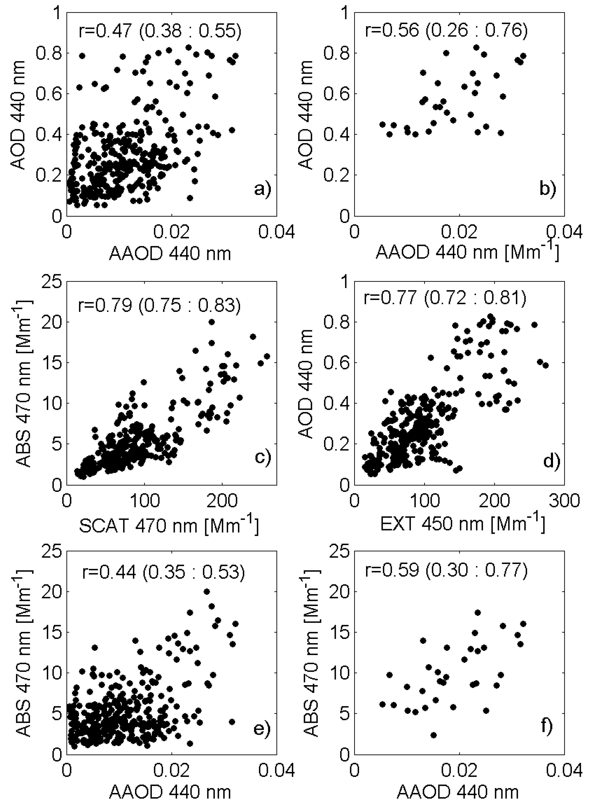
  • We found moderate correlation between AERONET AOD and AAOD (Pearson coefficient ≈0.47 ± 0.08 for lev. 1.5 and ≈0.56 ± 0.25 for lev. 2.0). AAOD correlated with ground in-situ absorption coefficient measurements gave very similar results (Pearson coefficient ≈0.44 ± 0.09 for lev. 1.5 and ≈0.59 ± 0.24 for lev. 2.0). However, significantly higher correlations were found for AOD with ground-based in-situ extinction coefficient (r ≈0.77 ± 0.05) and also for ground-based in-situ absorption and scattering (r ≈0.79 ± 0.04). AOD reported by AERONET is much better correlated with ground measurements of scattering and absorption (extinction) than AAOD. AAOD and AOD reported by AERONET over Strzyżów site were weakly correlated, despite high correlation of in-situ ground measurements of extinction and absorption coefficients.
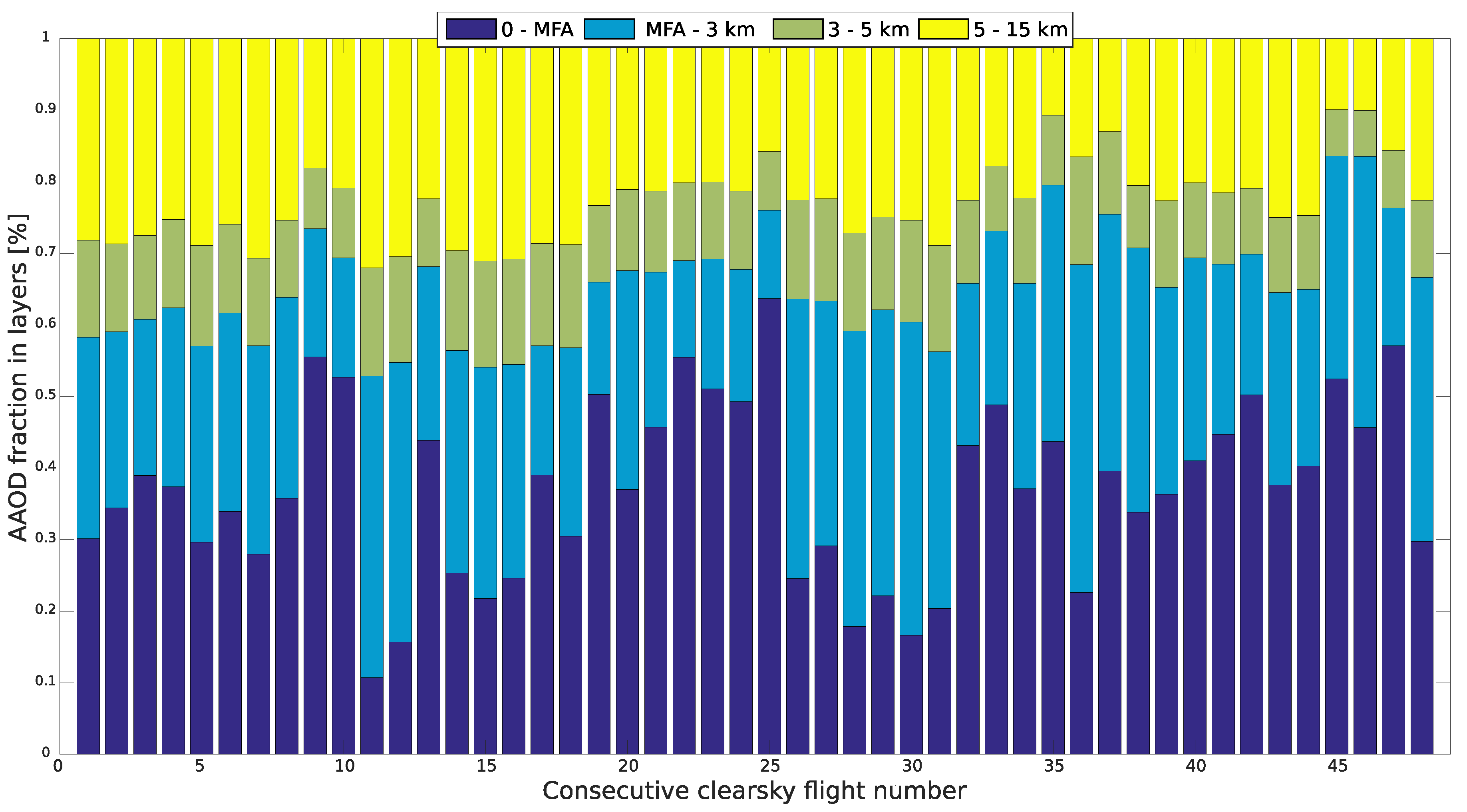
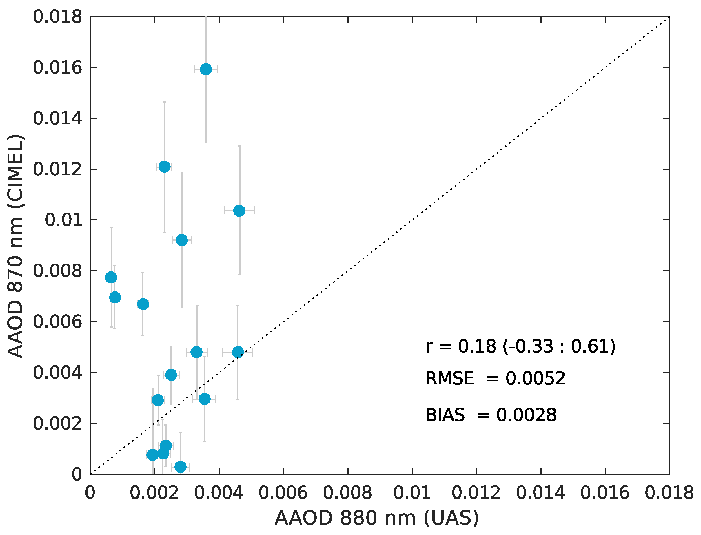
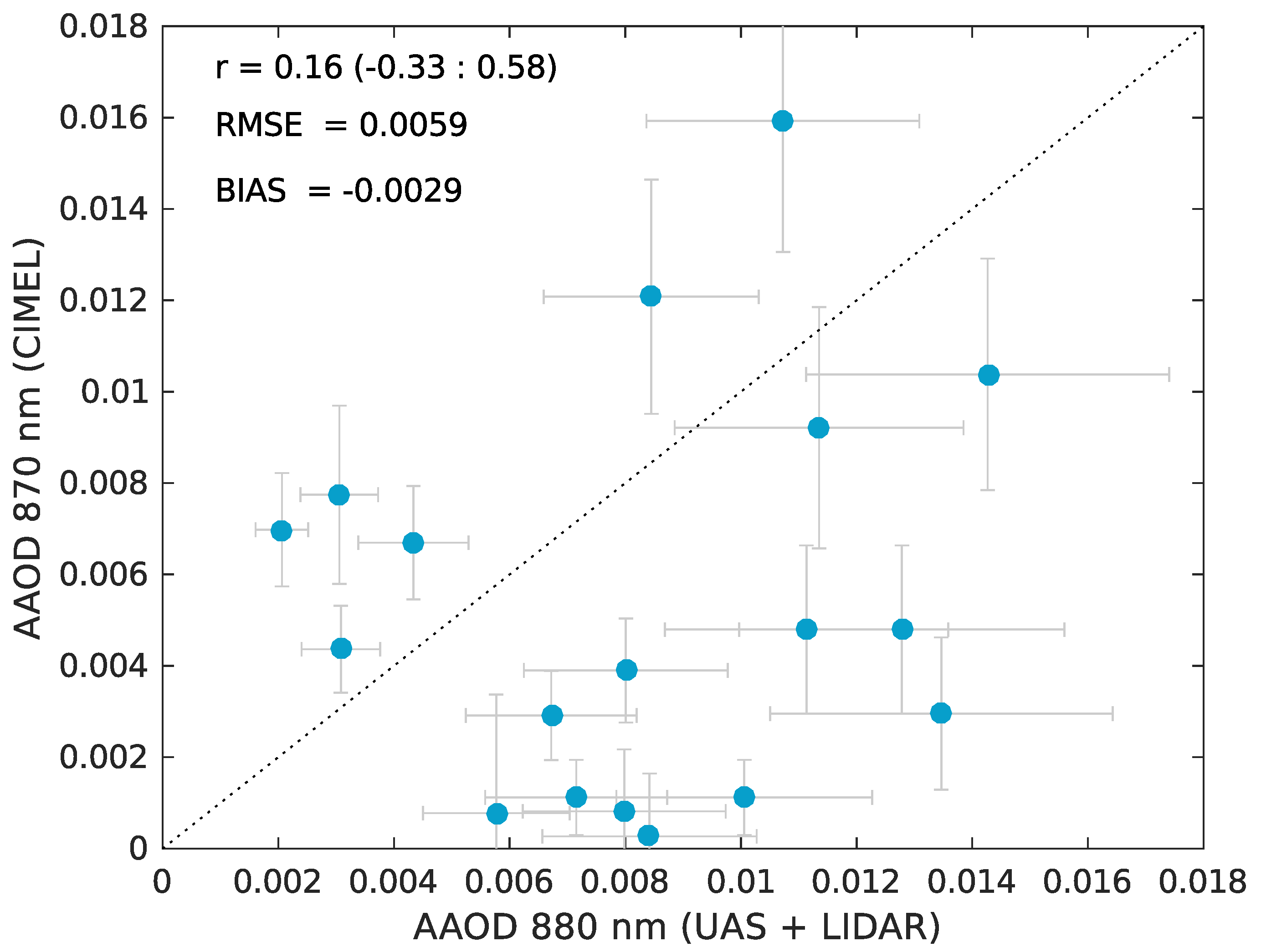
  • AAOD reported by AERONET was higher than measured from UAS (in the lowermost 1–1.5 km layer of the troposphere), which was expected due to a comparison of the whole atmosphere AAOD with one only in the lowest layer. There was no statistical correlation between measurements, however due to limited availability of data from AERONET estimations are insignificant. There were cases when AAOD measured in PBL was higher than reported by AERONET, which suggest possible underestimation of absorption in photometric measurements, under particular conditions. Based on lidar observations contribution of aerosols located in PBL to total AAOD was estimated to ≈37%.
  • AAOD measurements from drone correlating with ground-based measurements of absorption showed highest correlations (r ≈ 0.70) during daytime (06–18 UTC). Night time correlation was slightly lower (r ≈ 0.63). Results fit well into expectations, when during convective day conditions, mixing in PBL is stronger and difference between ground and PBL smaller. During night, especially if temperature inversion occurs, layered and inhomogeneous conditions are possible in PBL, which result in lower correlation with ground measurements.
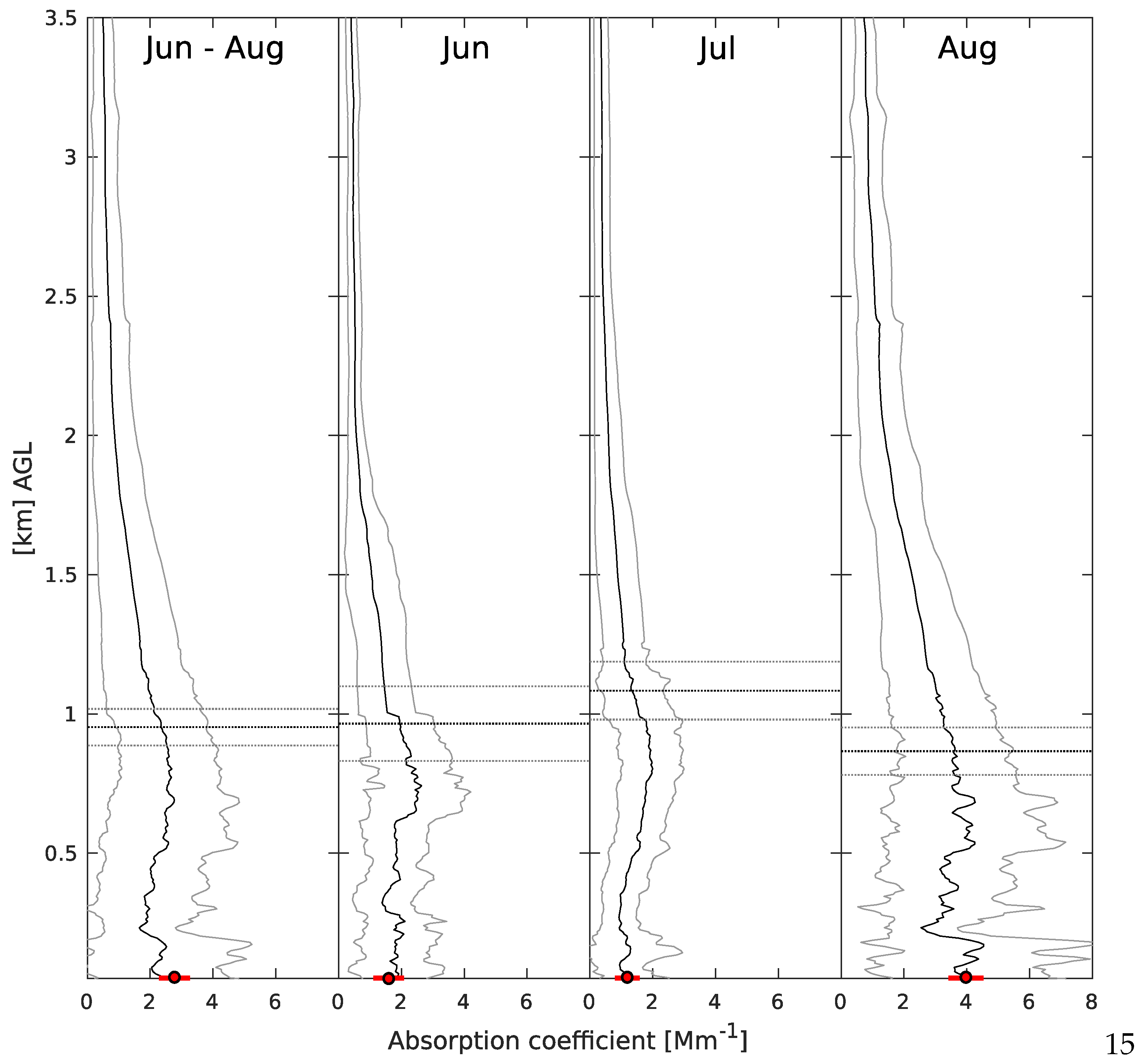
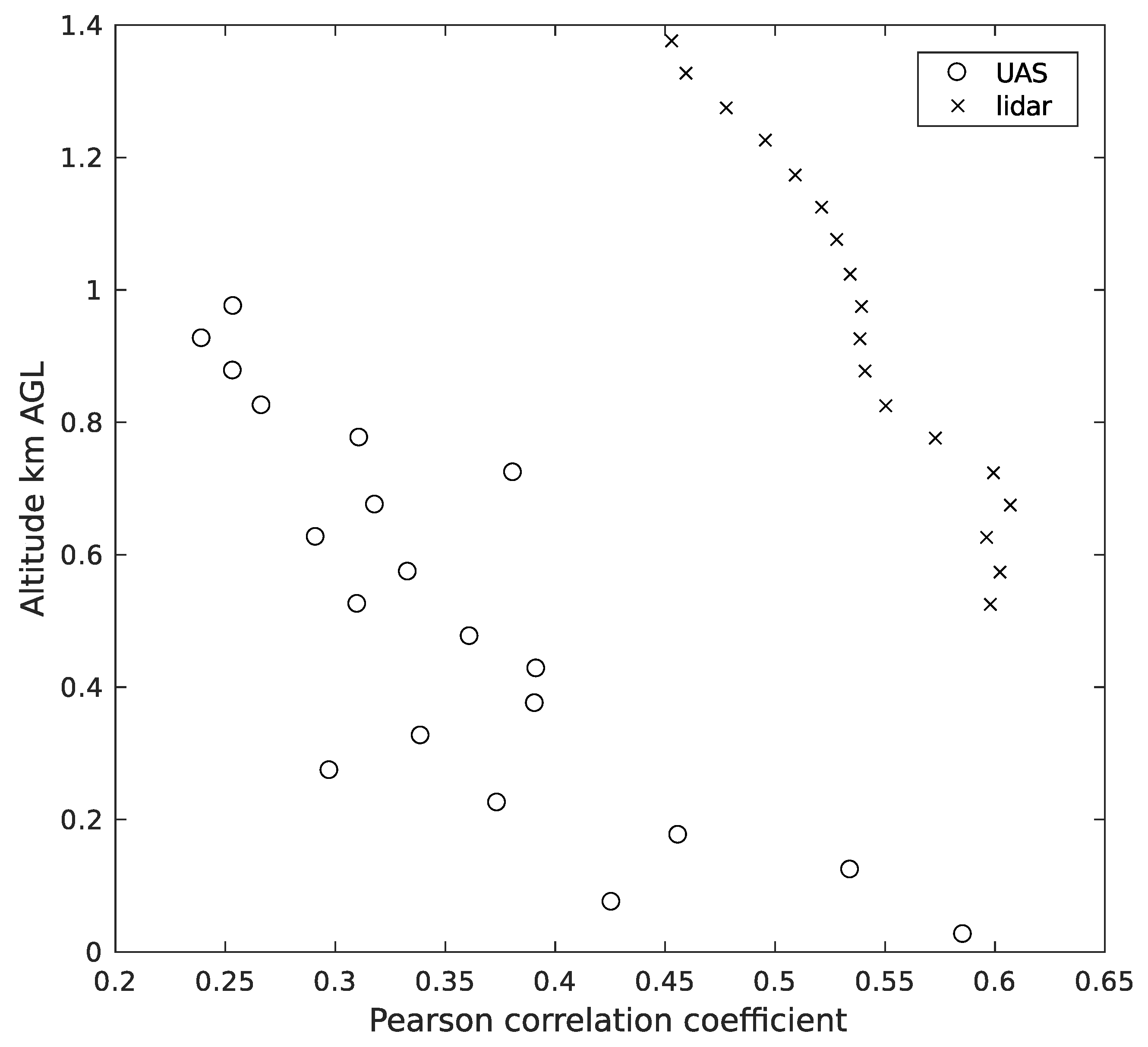
  • Correlation for the lower 500 m of profile (r ≈ 0.77 ± 0.10) with ground measurements was according to expectations much higher than correlation for layer above 500 m above ground (r ≈ 0.49 ± 0.18). Correlation of ground measurement with absorption in a layers decrease with altitude, which was checked for 21 layers in the range of UAS flight.
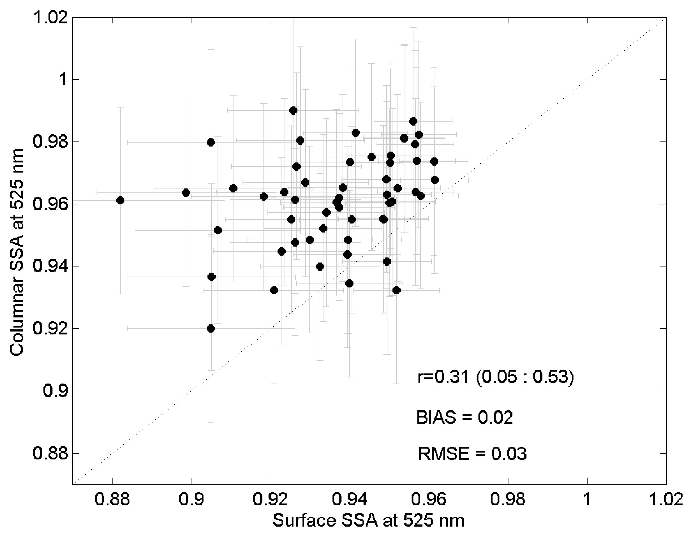
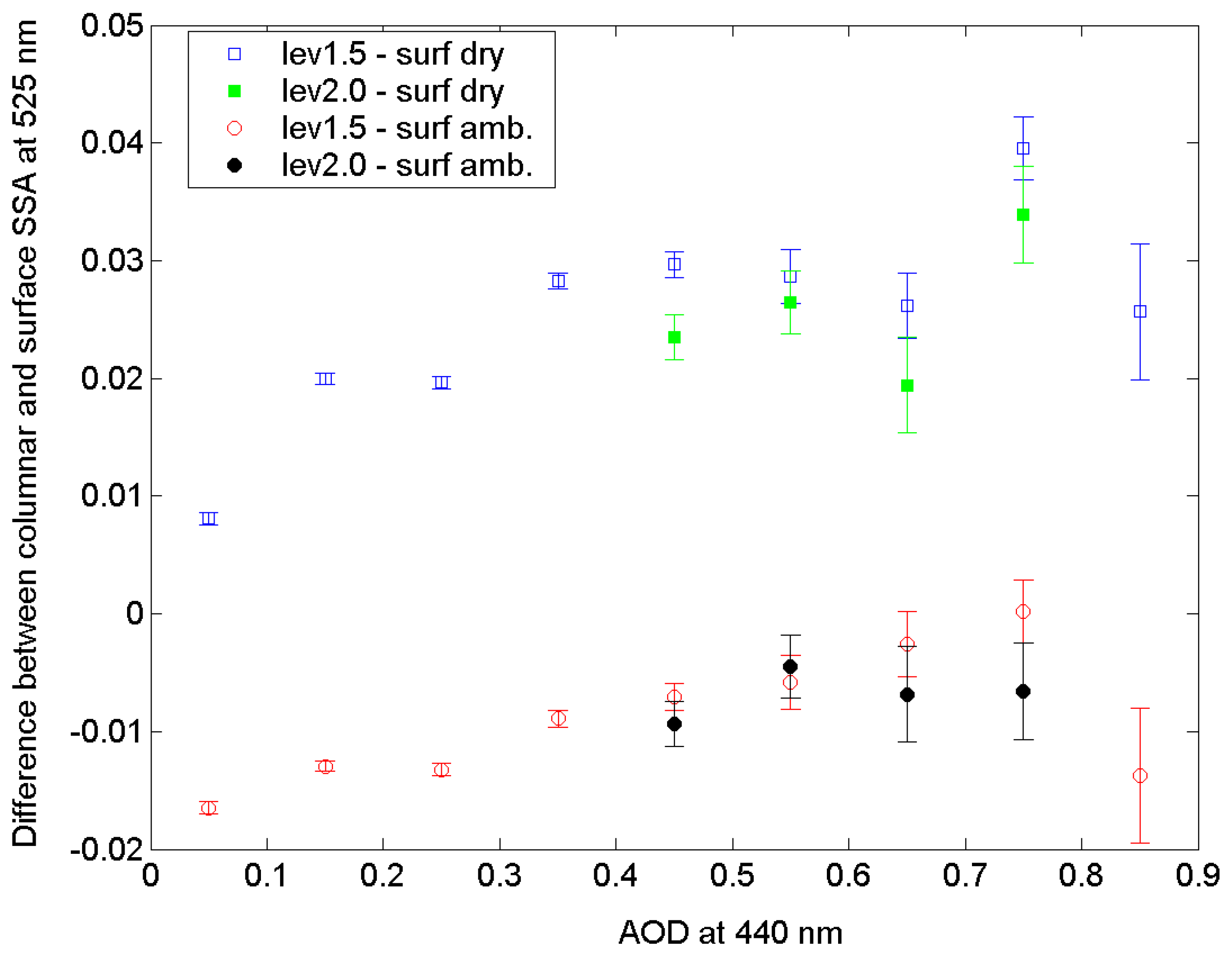
  • Comparison of SSA level 2.0 data from AERONET and surface in-situ SSA on 525 nm shows weak correlation and higher values of columnar data by ≈0.02, which mainly could be explained by hygroscopic effects. Ground measurements were done in dry conditions, while columnar data represent ambient conditions. For such reason correction for ambient condition with mean hygroscopic growth factor was applied. Correction reduced difference between both types of data. Difference is the smallest for AOD@441nm higher than 0.35 (≈0.005). This result confirms validity of using correction for ambient conditions.
  • Ground-based in-situ SSA measurements (aethalometer + nephelometer) and vertical in-situ SSA profiles (aethalometer on a drone + lidar) were juxtaposed with AERONET retrieval. Both in-situ methods with aethalometer gave quite similar mean values (≈0.92 ± 0.01 on ground and ≈0.92±0.02 in profile), with two times wider confidence interval for drone measurements. For the same period AERONET reported SSA at level ≈0.97 ± <0.01, which confirmed smaller contribution of absorption in AERONET retrieval in comparison to in-situ measurements.
  • Very limited availability of AERONET AAOD measurements was the reason for verification of simple methods for estimation of AAOD. Proposed methods base on AOD scaling by SSA retrieved from different methods (ground measurements, drone profiles and lidar/ceilometer data).
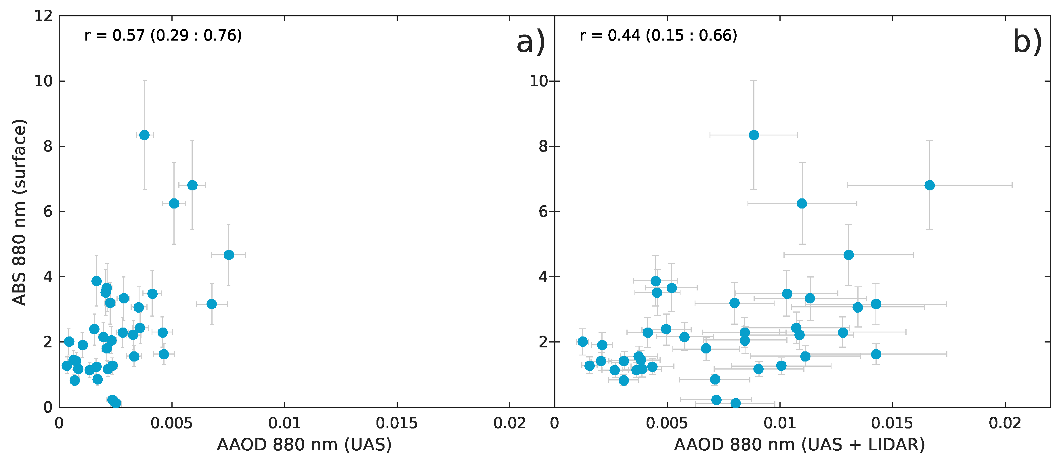
  • Obtained values of AAOD were correlated with AAOD delivered by AERONET and from combined drone and lidar measurement, but receiving statistically significant correlations for it was difficult due to small sample of AERONET data. Significant correlations were achieved for all estimations with AAOD measured from drone and lidar. The best correlation was achieved for AAOD estimated as AOD scaled by L SSA from lidar (r ≈ 0.94 ± 0.04) with lowest RMSE (0.0022). The weakest correlations were observed for methods with the integration of the absorption coefficient measured on the ground up to PBL/ABL (almost the same for both) with r ≈ 0.39 ± 0.27 and RMSE ≈ 0.0063. All AERONET correlations were insignificant, but it could be mentioned that the highest correlation coefficient was found for the integration of the absorption up to the PBL top (r ≈ 0.32).
Presented research show considerations on absorption coefficient profiles, AAOD and SSA retrievals with ground drones, lidars and ground measurements as solution for obtaining those values in case of insufficient amount of data from AERONET. Results confirms usability of remotely piloted aerial systems in aerosols research, especially in case of remote in-situ measurements of absorbing aerosols. Thanks to low UAS operation costs they could be used for more systematic observations of profiles, which could deliver valuable data for statistical analysis and verification of inter/in seasonal variability. Technological progress will improve range of UAS operations together with even better lidars systems for near field observations, which will make it possible to measure SSA profiles longer with less noise. In case of synchronized semi-automated systems it would be possible to make coordinated nearby flights, which will allow investigation of profiles spatial variability. Miniaturization of measurement devices could lead to development of micro-nephelometer, which will allow direct in-situ measurements of absorption and scattering coefficients vertical distribution (and SSA) from drones.
Despite that the measurement campaign took place in a very good measurement period (rainless, low fraction of cloud) AERONET AAOD data availability was very limited. For data from 2013–2017, AAOD data from level 2.0 is available only in 3% of cases, when AAOD 1.5 level data is available. Only 56 measurements were available at 2.0 level at SolarAOT station for 5 years of data collection. This AAOD level 2.0 data availability problem could be partially solved by data from level 1.5, when corresponding AOD for level 2.0 is defined.
The main conclusions on using AERONET absorption data are following:
  • For clean atmosphere there are high systematic uncertainties of AAOD and SSA on level 1.5 and there are no data for level 2.0. Therefore, for clean atmosphere (AOD below 0.2) there is overestimation of absorption on level 1.5, which results in the underestimation of SSA (0.946 on lev. 1.5 and 0.966 on lev. 2.0)
  • In five years, analysis mean AAOD from level 2.0 is overestimated due to threshold, whose filter cases with smaller amount of aerosols. For AAOD@441nm at SolarAOT station, values from level 2.0 (0.0182) are twice as high than for level 1.5 (0.0089).
  • Both levels are weakly correlated with in-situ measurements (ground and drone based). Additionally, results delivered by AERONET show, under particular conditions, possible underestimation of aerosols absorption. It was especially visible in cases where directly measured AAOD in PBL was higher than AAOD reported by AERONET. The mentioned issue is a premise for further investigation on the subject and further development of absorbing aerosols vertical profiling research, together with their results verification with collocated AERONET data.

Author Contributions

Conceptualization, M.T.C. and K.M.M.; data curation, M.T.C. and J.L. and O.Z.; funding acquisition, K.M.M. and I.S.S. (MULTIPLY project); investigation, M.T.C. and J.L. and P.M.; resources, I.S.S. (development of the lidar instrument NARLa); software, M.T.C.; supervision, K.M.M.; visualization, M.T.C. and J.L. and O.Z.; writing—original draft preparation, M.T.C.; writing—review and editing, I.S.S. and O.Z.

Funding

This research has been made within Polish Grant No. 2012/05/E/ST10/01578 of the National Science Centre coordinated by Institute of Geophysics, Faculty of Physics, University of Warsaw (IGFUW). The development of the algorithms used in this research were partly done in the frame of the POLIMOS project funded by the European Space Agency (ESA-ESTEC) uder Contract No. 4000119961/16/NL/FF/mg.

Acknowledgments

We would like to mention the support of AERONET-EUROPE/ACTRIS with calibration of the CIMEL at the SolarAOT station. The Near-range Aerosol Raman Lidar receiver (NARLa) was developed in the frame of scientific collaboration of IGFUW with Leibniz Institute for Tropospheric Research. Laboratory of Image-based information, Faculty of Biology, University of Warsaw helped with maintenance and preparation of UAS.

Conflicts of Interest

The authors declare no conflict of interest.

References

  1. IPCC. Climate Change 2013: The Physical Science Basis. Contribution of Working Group I to the Fifth Assessment Report of the Intergovernmental Panel on Climate Change; Cambridge University Press: Cambridge, UK; New York, NY, USA, 2013; p. 1535. [Google Scholar]
  2. Koch, D.; Del Genio, A.D. Black carbon semi-direct effects on cloud cover: Review and synthesis. Atmos. Chem. Phys. 2010, 10, 7685–7696. [Google Scholar] [CrossRef]
  3. Ramanathan, V.; Carmichael, G. Global and regional climate changes due to black carbon. Nat. Geosci. 2008, 1, 221–227. [Google Scholar] [CrossRef]
  4. Bond, T.C.; Doherty, S.J.; Fahey, D.W.; Forster, P.M.; Berntsen, T.; DeAngelo, B.J.; Flanner, M.G.; Ghan, S.; Karcher, B.; Koch, D.; et al. Bounding the role of black carbon in the climate system: A scientific assessment. J. Geophys. Res.-Atmos. 2013, 118, 5380–5552. [Google Scholar] [CrossRef]
  5. Samset, B.H.; Myhre, G.; Schulz, M.; Balkanski, Y.; Bauer, S.; Berntsen, T.K.; Bian, H.; Bellouin, N.; Diehl, T.; Easter, R.C.; et al. Black carbon vertical profiles strongly affect its radiative forcing uncertainty. Atmos. Chem. Phys. 2013, 13, 2423–2434. [Google Scholar] [CrossRef] [Green Version]
  6. Cook, J.; Highwood, E.J. Climate response to tropospheric absorbing aerosols in an intermediate general-circulation model. Q. J. R. Meteorol. Soc. 2004, 130, 175–191. [Google Scholar] [CrossRef] [Green Version]
  7. Choi, J.O.; Chung, C.E. Sensitivity of aerosol direct radiative forcing to aerosol vertical profile. Tellus Ser. B-Chem. Phys. Meteorol. 2014, 66. [Google Scholar] [CrossRef]
  8. Ban-Weiss, G.A.; Cao, L.; Bala, G.; Caldeira, K. Dependence of climate forcing and response on the altitude of black carbon aerosols. Clim. Dyn. 2012, 38, 897–911. [Google Scholar] [CrossRef]
  9. Meloni, D.; di Sarra, A.; Di Iorio, T.; Fiocco, G. Influence of the vertical profile of Saharan dust on the visible direct radiative forcing. J. Quant. Spectrosc. Radiat. Transf. 2005, 93, 397–413. [Google Scholar] [CrossRef]
  10. Johnson, B.T.; Heese, B.; McFarlane, S.A.; Chazette, P.; Jones, A.; Bellouin, N. Vertical distribution and radiative effects of mineral dust and biomass burning aerosol over West Africa during DABEX. J. Geophys. Res.-Atmos. 2008, 113. [Google Scholar] [CrossRef]
  11. Gomez-Amo, J.L.; di Sarra, A.; Meloni, D.; Cacciani, M.; Utrillas, M.P. Sensitivity of shortwave radiative fluxes to the vertical distribution of aerosol single scattering albedo in the presence of a desert dust layer. Atmos. Environ. 2010, 44, 2787–2791. [Google Scholar] [CrossRef]
  12. Holben, B.N.; Eck, T.F.; Slutsker, I.; Tanre, D.; Buis, J.P.; Setzer, A.; Vermote, E.; Reagan, J.A.; Kaufman, Y.J.; Nakajima, T.; et al. AERONET–A federated instrument network and data archive for aerosol characterization. Remote Sens. Environ. 1998, 66, 1–16. [Google Scholar] [CrossRef]
  13. Dubovik, O.; King, M.D. A flexible inversion algorithm for retrieval of aerosol optical properties from Sun and sky radiance measurements. J. Geophys. Res.-Atmos. 2000, 105, 20673–20696. [Google Scholar] [CrossRef] [Green Version]
  14. Andrews, E.; Ogren, J.A.; Kinne, S.; Samset, B. Comparison of AOD, AAOD and column single scattering albedo from AERONET retrievals and in situ profiling measurements. Atmos. Chem. Phys. 2017, 17, 6041–6072. [Google Scholar] [CrossRef] [Green Version]
  15. Schafer, J.S.; Eck, T.F.; Holben, B.N.; Thornhill, K.L.; Anderson, B.E.; Sinyuk, A.; Giles, D.M.; Winstead, E.L.; Ziemba, L.D.; Beyersdorf, A.J.; et al. Intercomparison of aerosol single-scattering albedo derived from AERONET surface radiometers and LARGE in situ aircraft profiles during the 2011 DRAGON-MD and DISCOVER-AQ experiments. J. Geophys. Res.-Atmos. 2014, 119, 7439–7452. [Google Scholar] [CrossRef] [Green Version]
  16. Saturno, J.; Pohlker, C.; Massabo, D.; Brito, J.; Carbone, S.; Cheng, Y.F.; Chi, X.G.; Ditas, F.; de Angelis, I.H.; Moran-Zuloaga, D.; et al. Comparison of different Aethalometer correction schemes and a reference multi-wavelength absorption technique for ambient aerosol data. Atmos. Meas. Tech. 2017, 10, 2837–2850. [Google Scholar] [CrossRef] [Green Version]
  17. Weingartner, E.; Saathoff, H.; Schnaiter, M.; Streit, N.; Bitnar, B.; Baltensperger, U. Absorption of light by soot particles: determination of the absorption coefficient by means of aethalometers. J. Aerosol Sci. 2003, 34, 1445–1463. [Google Scholar] [CrossRef]
  18. Schmid, O.; Artaxo, P.; Arnott, W.P.; Chand, D.; Gatti, L.V.; Frank, G.P.; Hoffer, A.; Schnaiter, M.; Andreae, M.O. Spectral light absorption by ambient aerosols influenced by biomass burning in the Amazon Basin. I: Comparison and field calibration of absorption measurement techniques. Atmos. Chem. Phys. 2006, 6, 3443–3462. [Google Scholar] [CrossRef] [Green Version]
  19. White, W.H.; Trzepla, K.; Hyslop, N.P.; Schichtel, B.A. A critical review of filter transmittance measurements for aerosol light absorption, and de novo calibration for a decade of monitoring on PTFE membranes. Aerosol Sci. Technol. 2016, 50, 984–1002. [Google Scholar] [CrossRef]
  20. Coen, M.C.; Weingartner, E.; Apituley, A.; Ceburnis, D.; Fierz-Schmidhauser, R.; Flentje, H.; Henzing, J.S.; Jennings, S.G.; Moerman, M.; Petzold, A.; et al. Minimizing light absorption measurement artifacts of the Aethalometer: Evaluation of five correction algorithms. Atmos. Meas. Tech. 2010, 3, 457–474. [Google Scholar] [CrossRef]
  21. Bueno, P.A.; Havey, D.K.; Mulholland, G.W.; Hodges, J.T.; Gillis, K.A.; Dickerson, R.R.; Zachariah, M.R. Photoacoustic Measurements of Amplification of the Absorption Cross Section for Coated Soot Aerosols. Aerosol Sci. Technol. 2011, 45, 1217–1230. [Google Scholar] [CrossRef]
  22. Markowicz, K.M.; Ritter, C.; Lisok, J.; Makuch, P.; Stachlewska, I.S.; Cappelletti, D.; Mazzola, M.; Chilinski, M.T. Vertical variability of aerosol single-scattering albedo and equivalent black carbon concentration based on in-situ and remote sensing techniques during the iAREA campaigns in Ny-Alesund. Atmos. Environ. 2017, 164, 431–447. [Google Scholar] [CrossRef]
  23. Ferrero, L.; Cappelletti, D.; Busetto, M.; Mazzola, M.; Lupi, A.; Lanconelli, C.; Becagli, S.; Traversi, R.; Caiazzo, L.; Giardi, F.; et al. Vertical profiles of aerosol and black carbon in the Arctic: A seasonal phenomenology along 2 years (2011-2012) of field campaigns. Atmos. Chem. Phys. 2016, 16, 12601–12629. [Google Scholar] [CrossRef]
  24. Villa, T.F.; Gonzalez, F.; Miljievic, B.; Ristovski, Z.D.; Morawska, L. An Overview of Small Unmanned Aerial Vehicles for Air Quality Measurements: Present Applications and Future Prospectives. Sensors 2016, 16. [Google Scholar] [CrossRef] [PubMed]
  25. Corrigan, C.E.; Roberts, G.C.; Ramana, M.V.; Kim, D.; Ramanathan, V. Capturing vertical profiles of aerosols and black carbon over the Indian Ocean using autonomous unmanned aerial vehicles. Atmos. Chem. Phys. 2008, 8, 737–747. [Google Scholar] [CrossRef] [Green Version]
  26. Chilinski, M.T.; Markowicz, K.M.; Markowicz, J. Observation of vertical variability of black carbon concentration in lower troposphere on campaigns in Poland. Atmos. Environ. 2016, 137, 155–170. [Google Scholar] [CrossRef]
  27. Chiliński, M.T.; Markowicz, K.M.; Kubicki, M. UAS as a Support for Atmospheric Aerosols Research: Case Study. Pure Appl. Geophys. 2018. [Google Scholar] [CrossRef]
  28. Muller, D.; Wandinger, U.; Ansmann, A. Microphysical particle parameters from extinction and backscatter lidar data by inversion with regularization: theory. Appl. Opt. 1999, 38, 2346–2357. [Google Scholar] [CrossRef] [PubMed]
  29. Veselovskii, I.; Kolgotin, A.; Griaznov, V.; Muller, D.; Wandinger, U.; Whiteman, D.N. Inversion with regularization for the retrieval of tropospheric aerosol parameters from multiwavelength lidar sounding. Appl. Opt. 2002, 41, 3685–3699. [Google Scholar] [CrossRef] [PubMed] [Green Version]
  30. Veselovskii, I.; Kolgotin, A.; Griaznov, V.; Muller, D.; Franke, K.; Whiteman, D.N. Inversion of multiwavelength Raman lidar data for retrieval of bimodal aerosol size distribution. Appl. Opt. 2004, 43, 1180–1195. [Google Scholar] [CrossRef]
  31. Kolgotin, A.; Muller, D. Theory of inversion with two-dimensional regularization: Profiles of microphysical particle properties derived from multiwavelength lidar measurements. Appl. Opt. 2008, 47, 4472–4490. [Google Scholar] [CrossRef]
  32. Chaikovsky, A.; Dubovik, O.; Holben, B.; Bril, A.; Goloub, P.; Tanre, D.; Pappalardo, G.; Wandinger, U.; Chaikovskaya, L.; Denisov, S.; et al. Lidar-Radiometer Inversion Code (LIRIC) for the retrieval of vertical aerosol properties from combined lidar/radiometer data: Development and distribution in EARLINET. Atmos. Meas. Tech. 2016, 9, 1181–1205. [Google Scholar] [CrossRef]
  33. Tsekeri, A.; Amiridis, V.; Lopatin, A.; Marinou, E.; Giannakaki, E.; Pikridas, M.; Sciare, J.; Liakakou, E.; Gerasopoulos, E.; Duesing, S.; et al. Aerosol absorption profiling from the synergy of lidar and sun-photometry: The ACTRIS-2 campaigns in Germany, Greece and Cyprus. EPJ Web Conf. 2018, 176, 08005. [Google Scholar] [CrossRef]
  34. Hansen, A.D.A.; Rosen, H.; Novakov, T. The aethalometer–an instrument for the real-time measurement of optical-absorption by aerosol-particles. Sci. Total Environ. 1984, 36, 191–196. [Google Scholar] [CrossRef]
  35. Segura, S.; Estelles, V.; Titos, G.; Lyamani, H.; Utrillas, M.P.; Zotter, P.; Prevot, A.S.H.; Mocnik, G.; Alados-Arboledas, L.; Martinez-Lozano, J.A. Determination and analysis of in situ spectral aerosol optical properties by a multi-instrumental approach. Atmos. Meas. Tech. 2014, 7, 2373–2387. [Google Scholar] [CrossRef] [Green Version]
  36. Chamberlain-Ward, S.; Sharp, F. Advances in Nephelometry through the Ecotech Aurora Nephelometer. Sci. World J. 2011, 11, 2530–2535. [Google Scholar] [CrossRef] [PubMed]
  37. Muller, T.; Laborde, M.; Kassell, G.; Wiedensohler, A. Design and performance of a three-wavelength LED-based total scatter and backscatter integrating nephelometer. Atmos. Meas. Tech. 2011, 4, 1291–1303. [Google Scholar] [CrossRef] [Green Version]
  38. Anderson, T.L.; Ogren, J.A. Determining Aerosol Radiative Properties Using the TSI 3563 Integrating Nephelometer. Aerosol Sci. Technol. 1998, 29, 57–69. [Google Scholar] [CrossRef] [Green Version]
  39. Truex, T.J.; Anderson, J.E. Mass monitoring of carbonaceous aerosols with a spectrophone. Atmos. Environ. 1979, 13, 507–509. [Google Scholar] [CrossRef]
  40. Stachlewska, I.S.; Markowicz, K.M.; Ritter, C.; Neuber, R.; Heese, B.; Engelmann, R.; Linne, H. Near-range receiver unit of next generation pollyxt used with koldeway aerosol raman lidar in arctic. EPJ Web Conf. 2016, 119, 06015. [Google Scholar] [CrossRef]
  41. Engelmann, R.; Kanitz, T.; Baars, H.; Heese, B.; Althausen, D.; Skupin, A.; Wandinger, U.; Komppula, M.; Stachlewska, I.S.; Amiridis, V.; et al. The automated multiwavelength Raman polarization and water-vapor lidar Polly(XT): The neXT generation. Atmos. Meas. Tech. 2016, 9, 1767–1784. [Google Scholar] [CrossRef]
  42. Klett, J.D. Stable analytical inversion solution for processing lidar returns. Appl. Opt. 1981, 20, 211–220. [Google Scholar] [CrossRef] [Green Version]
  43. Klett, J.D. Lidar inversion with variable backscatter extinction ratios. Appl. Opt. 1985, 24, 1638–1643. [Google Scholar] [CrossRef]
  44. Fernald, F.G. Analysis of atmospheric lidar observations - some comments. Appl. Opt. 1984, 23, 652–653. [Google Scholar] [CrossRef]
  45. Stachlewska, I.S.; Piadlowski, M.; Migacz, S.; Szkop, A.; Zielinska, A.J.; Swaczyna, P.L. Ceilometer Observations of the Boundary Layer over Warsaw, Poland. Acta Geophys. 2012, 60, 1386–1412. [Google Scholar] [CrossRef]
  46. Markowicz, K.M.; Chilinski, M.T.; Lisok, J.; Zawadzka, O.; Stachlewska, I.S.; Janicka, L.; Rozwadowska, A.; Makuch, P.; Pakszys, P.; Zielinski, T.; et al. Study of aerosol optical properties during long-range transport of biomass burning from Canada to Central Europe in July 2013. J. Aerosol Sci. 2016, 101, 156–173. [Google Scholar] [CrossRef]
  47. Giles, D.M.; Sinyuk, A.; Sorokin, M.G.; Schafer, J.S.; Smirnov, A.; Slutsker, I.; Eck, T.F.; Holben, B.N.; Lewis, J.R.; Campbell, J.R.; et al. Advancements in the Aerosol Robotic Network (AERONET) Version 3 database–automated near-real-time quality control algorithm with improved cloud screening for Sun photometer aerosol optical depth (AOD) measurements. Atmos. Meas. Tech. 2019, 12, 169–2019. [Google Scholar] [CrossRef]
  48. Hagler, G.S.W.; Yelverton, T.L.B.; Vedantham, R.; Hansen, A.D.A.; Turner, J.R. Post-processing Method to Reduce Noise while Preserving High Time Resolution in Aethalometer Real-time Black Carbon Data. Aerosol Air Qual. Res. 2011, 11, 539–546. [Google Scholar] [CrossRef] [Green Version]
  49. Arnott, W.P.; Hamasha, K.; Moosmuller, H.; Sheridan, P.J.; Ogren, J.A. Towards aerosol light-absorption measurements with a 7-wavelength Aethalometer: Evaluation with a photoacoustic instrument and 3-wavelength nephelometer. Aerosol Sci. Technol. 2005, 39, 17–29. [Google Scholar] [CrossRef]
  50. Ferrero, L.; Mocnik, G.; Ferrini, B.S.; Perrone, M.G.; Sangiorgi, G.; Bolzacchini, E. Vertical profiles of aerosol absorption coefficient from micro-Aethalometer data and Mie calculation over Milan. Sci. Total Environ. 2011, 409, 2824–2837. [Google Scholar] [CrossRef]
  51. Ran, L.; Deng, Z.Z.; Xu, X.B.; Yan, P.; Lin, W.L.; Wang, Y.; Tian, P.; Wang, P.C.; Pan, W.L.; Lu, D.R. Vertical profiles of black carbon measured by a micro-aethalometer in summer in the North China Plain. Atmos. Chem. Phys. 2016, 16, 10441–10454. [Google Scholar] [CrossRef] [Green Version]
  52. Janicka, L.; Stachlewska, I.S. Properties of biomass burning aerosol mixtures derived at fine temporal and spatial scales from Raman lidar measurements: Part I optical properties. Atmos. Chem. Phys. Discuss. 2019, 1–46. [Google Scholar] [CrossRef]
  53. Janicka, L.; Stachlewska, I.S.; Veselovskii, I.; Baars, H. Temporal variations in optical and microphysical properties of mineral dust and biomass burning aerosol derived from daytime Raman lidar observations over Warsaw, Poland. Atmos. Environ. 2017, 169, 162–174. [Google Scholar] [CrossRef]
  54. Stachlewska, I.S.; Costa-Surós, M.; Althausen, D. Raman lidar water vapor profiling over Warsaw, Poland. Atmos. Res. 2017, 194, 258–267. [Google Scholar] [CrossRef]
  55. Brooks, I.M. Finding boundary layer top: Application of a wavelet covariance transform to lidar backscatter profiles. J. Atmos. Ocean. Technol. 2003, 20, 1092–1105. [Google Scholar] [CrossRef]
  56. Baars, H.; Ansmann, A.; Engelmann, R.; Althausen, D. Continuous monitoring of the boundary-layer top with lidar. Atmos. Chem. Phys. 2008, 8, 7281–7296. [Google Scholar] [CrossRef] [Green Version]
  57. Seibert, P.; Beyrich, F.; Gryning, S.E.; Joffre, S.; Rasmussen, A.; Tercier, P. Review and intercomparison of operational methods for the determination of the mixing height. Atmos. Environ. 2000, 34, 1001–1027. [Google Scholar] [CrossRef]
  58. Zhang, L.; Henze, D.K.; Grell, G.A.; Torres, O.; Jethva, H.; Lamsal, L.N. What factors control the trend of increasing AAOD over the United States in the last decade? J. Geophys. Res. Atmos. 2017, 122, 1797–1810. [Google Scholar] [CrossRef]
  59. Konovalov, I.B.; Lvova, D.A.; Beekmann, M.; Jethva, H.; Mikhailov, E.F.; Paris, J.D.; Belan, B.D.; Kozlov, V.S.; Ciais, P.; Andreae, M.O. Estimation of black carbon emissions from Siberian fires using satellite observations of absorption and extinction optical depths. Atmos. Chem. Phys. 2018, 18, 14889–14924. [Google Scholar] [CrossRef] [Green Version]
  60. Szczepanik, D.; Markowicz, K.M. The relation between columnar and surface aerosol optical properties in a background environment. Atmos. Pollut. Res. 2018, 9, 246–256. [Google Scholar] [CrossRef]
  61. Zawadzka, O.; Markowicz, K.; Pietruczuk, A.; Zielinski, T.; Jaroslawski, J. Impact of urban pollution emitted in Warsaw on aerosol properties. Atmos. Environ. 2013, 69, 15–28. [Google Scholar] [CrossRef]
Figure 1. Location of the Poland-AOD (network) station in Strzyżów
Atmosphere 10 00446 g001
Figure 2. Versa X6 multicopter with scientific payload (AE-51 aethalometer and radiosonde RS92-SGP).
Atmosphere 10 00446 g002
Figure 3. Comparison of AE-51 attenuation coefficient at 880 nm and aerosol absorption coefficient at 870 nm from photoacoustic extinctiometer (PAX) obtained between 29 June and 1 July of 2016. Black dots represent one-hour average data while the solid line is a linear fit.
Atmosphere 10 00446 g003
Figure 4. Comparison of (a) the attenuation and (b) absorption coefficients obtained from AE-31 and AE-51 during field campaign at SolarAOT in 2015. Solid line indicates linear fit and dotted line shows perfect agreement.
Atmosphere 10 00446 g004
Figure 5. Changes in signal-to-noise ratio (SNR) for channels 532 nm and 607 nm of near-range aerosol Raman lidar (NARLa) at 1 km height on 03/08/2015 at SolarAOT site.
Atmosphere 10 00446 g005
Figure 6. Difference between AOD measurement made by CIMEL-318 before sunset and after sunrise on SolarAOT site (AERONET data 2013–2017).
Atmosphere 10 00446 g006
Figure 7. Fraction of absorbing aerosol optical depth (AAOD) in layers. Estimation based on unmanned aerial system (UAS) measurements scaled with lidar derived extinction and measured SSA. Profiles acquired during June–August 2015 at SolarAOT site. MFA—maximum flight altitude of UAS.
Atmosphere 10 00446 g007
Figure 8. Comparison of (a) Aerosol Robotic Network (AERONET) Level 1.5 (317 cases) and (b) 2.0 (33 cases) AAOD and AOD, (c) surface absorption (aethalometer) and scattering (nephelometer) coefficient, (d) surface extinction (aethalometer + nephelometer) and columnar AOD, (e) AERONET level 1.5 and (f) 2.0 AAOD with surface absorption (aethalometer) coefficient measured between June and August 2015 at SolarAOT site.
Atmosphere 10 00446 g008
Figure 9. Comparison of columnar (Level 2.0 AERONET) and surface single scattering albedo (SSA) (aethalometer + nephelometer) at 525 nm. Grey error bars show uncertainties. Dashed line (x = y) only for a reference.
Atmosphere 10 00446 g009
Figure 10. Difference between columnar and surface SSA (aethalometer + nephelometer) at 525 nm as a function of AOD at 440 nm for Level 1.5 AERONET data at dry (blues squares) and ambient conditions (red circles) as well as for Level 2.0 AERONET data and at dry (green solid squares) and ambient conditions (black dotted). The error bars marks the uncertainties related to number of measurements (0.01/ N ).
Atmosphere 10 00446 g010
Figure 11. Comparison of the AAOD@870 nm obtained from level 1.5 AERONET data against AAOD@880 nm measured by UAS profiling during June–August 2015 at SolatAOT site [18 cases]. Grey error bars show uncertainties. Dashed line (x = y) only for a reference.
Atmosphere 10 00446 g011
Figure 12. Comparison of the AAOD@870 nm obtained from the Level 1.5 AERONET data against AAOD@880 nm from UAS profiles extended with lidar observations during June–August 2015 at SolatAOT site (18 cases). Grey error bars show uncertainties. Dashed line (x = y) only for a reference.
Atmosphere 10 00446 g012
Figure 13. Scatter plot for surface absorption (aethalometer) coefficient at 880 nm and AAOD@880nm estimated from (a) UAS profiles and (b) UAS profiles extended by lidar measurements in June–August 2015 at SolarAOT site.
Atmosphere 10 00446 g013
Figure 14. Averaged absorption coefficient profiles measured from UAS during summer campaign at SolarAOT site in 2015. Vertical grey lines indicate 95% confidence intervals for mean. Dotted lines represent PBL height with corresponding 95% confidence intervals. Ground values measured by aethalometer AE-31 are marked by red dots on axis with red lines as confidence interval.
Atmosphere 10 00446 g014
Figure 15. Change of Pearson correlation coefficient with altitude for 1) absorption coefficient measured on ground by AE-31 and absorption coefficient measured by AE-51 on the UAS, 2) extinction coefficient retrieved from lidar measurements.
Atmosphere 10 00446 g015
Figure 16. AAOD approximated by different methods.
Atmosphere 10 00446 g016
Table 1. Mean aerosol optical properties between June and August 2015 at SolarAOT station for in-situ (aethalometer + nephelometer) and Aerosol Robotic Network (AERONET) level 1.5 and 2.0 and four wavelengths (440, 525, 675, and 870 nm). A O D d i r e c t and A O D r e t corresponds to direct and inversion product, absorbing aerosol optical depth (AAOD) and single scattering albedo (SSA) are AERONET retrievals while S S A s u r f ( R H d r y ), S S A s u r f ( R H a m b i e n t ), S S A s u r f (<RH>) are surface SSA for dry, ambient and mean RH in the aerosol mixing layer, respectively.
AERONET Level 1.5AERONET Level 2.0
[nm]440525675870440525675870
AOD d i r e c t ----0.2800.2160.1340.086
AOD r e t 0.2880.2130.1390.090.5710.4210.2730.168
AAOD0.0110.010.0080.0070.0180.0150.0120.01
SSA0.9550.9470.9340.9140.9670.9620.9540.939
SSA s u r f [RH d r y ]0.9380.9390.9320.9280.9420.9420.9340.929
SSA s u r f [RH a m b i e n t ]0.9470.9480.9420.9380.9530.9530.9460.942
SSA s u r f [<RH>]0.9650.9660.9620.9590.9700.9710.9660.964
Table 2. Absorption coefficient measured on ground (AE-31), in profiles (AE-51 on unmanned aerial system (UAS)) and AOD during June–August 2015. For AOD and ground measurements monthly anomaly is calculated. Mean values for profiles are presented with confidence intervals and in brackets with Pearson correlation coefficient to ground measurements.
Absorption Coefficient on Ground + Anomaly (2013–2017)
Absorption [Mm 1 ]June–AugustJuneJulyAugust
ABS@520 nm3.803.002.605.80
dABS@520 nm+0.70+0.43−0.04+1.72
ABS@870 nm2.011.411.413.04
dABS@870 nm+0.32+0.11−0.05+0.89
AERONET AOD@500 nm + 2013–2017 + Anomaly
AODJune–AugustJuneJulyAugust
2013–20170.1860.1800.1790.196
20150.2330.2020.1890.282
dAOD+0.05+0.02+0.01+0.09
Absorption Coefficient during Flights in 2015
Absorption [Mm 1 ]All ProfilesJuneJulyAugust
on ground2.74 ± 0.42 [1.00]1.73 ± 0.33 [1.00]1.25 ± 0.14 [1.00]3.95 ± 0.58 [1.00]
profile mean2.78 ± 0.33 [0.67 ± 0.13]1.80 ± 0.58 [—]1.51 ± 0.27 [ — ]3.78 ± 0.34 [0.73 ± 0.11]
lower 500 m2.62 ± 0.35 [0.77 ± 0.10]1.62 ± 0.53 [—]1.15 ± 0.24 [ — ]3.74 ± 0.34 [0.79 ± 0.09]
upper 500 m3.01 ± 0.35 [0.49 ± 0.18]2.26 ± 0.79 [—]1.86 ± 0.33 [ — ]3.85 ± 0.44 [0.65 ± 0.13]
Table 3. Single scattering albedo measured/retrieved by different methods. Mean value with confidence intervals and standard deviations are presented. L Single scattering albedo (SSA) values are obtained with described in Section 3.2 method with extinction coefficient retrieved from different remote sensing systems (lidar, ceilometer).
Source of SSA MeasurementMean SSAstd
Aethelomter + nephelometer on ground0.923 ± 0.0060.020
UAS (AE-51) + Lidar0.917 ± 0.0160.056
L SSA Lidar0.869 ± 0.0250.085
L SSA Ceilometer0.840 ± 0.0340.115
AERONET0.974 ± 0.0020.003
Table 4. Correlation coefficient between AERONET AAOD or AAOD approximated from UAS + lidar measurements and different AAOD approximation methods. 95% confidence intervals for correlation are presented in square brackets. Significant Pearson correlation coefficients are presented in bold. Root mean squared error (RMSE) and bias for linear fit with relation to the mean value shown in brackets (in blue when values are below 40% of the mean value).
Only Common Points of AERONET
AERONETUAS + LIDAR
rRMSEbiasrRMSEbias
Surface SSA0.42 [−0.06:0.74]0.0041 (0.75)0.0011 (0.21)0.34 [−0.15:0.7]0.0053 (0.64)0.004 (0.49)
Surface SSA w e t 0.42 [−0.06:0.74]0.0043 (0.81)0.002 (0.37)0.19 [−0.3:0.61]0.0061 (0.74)0.0049 (0.59)
Drone SSA−0.05 [−0.51:0.43]0.0072 (1.33)−0.0043 (−0.81)0.77 [0.48:0.91]0.0028 (0.34)−0.0014 (−0.17)
Drone SSA w e t −0.05 [−0.51:0.43]0.0058 (1.08)−0.0026 (−0.48)0.67 [0.3:0.87]0.0027 (0.32)0.0003 (0.04)
L SSA Lidar0.25 [−0.25:0.64]0.0071 (1.32)−0.0038 (−0.70)0.9 [0.74:0.96]0.0029 (0.35)−0.0009 (0.04)
L SSA Ceilometer0.006 [−0.42:51]0.0106 (1.98)−0.0063 (−1.16)0.79 [0.51:0.92]0.0063 (0.77)−0.0034 (−0.41)
ABS to PBL0.36 [−0.13:0.71]0.0056 (1.04)0.0038 (0.70)0.22 [−0.28:0.62]0.0075 (0.91)0.0067 (0.81)
ABS to ABL−0.01 [−0.48:0.46]0.0005 (0.99)0.0028 (0.53)0.28 [−0.22:0.66]0.0067 (0.81)0.00057 (0.69)
UAS + Ceilometer0.36 [−0.13:0.71]0.0040 (0.75)0.0008 (0.14)0.66 [0.27:0.86]0.0046 (0.55)0.0037 (0.44)
All Data Points
AERONETUAS + LIDAR
rRMSEBIASrRMSEBIAS
Surface SSA0.09 [−0.34:0.48]0.0051 (0.96)0.0004 (0.07)0.55 [0.29:0.74]0.0043 (0.58)0.0025 (0.34)
Surface SSA w e t 0.07 [−0.35:0.47]0.0045 (0.96)0.0012 (0.23)0.49 [0.21:0.7]0.005 (0.67)0.0035 (0.47)
Drone SSA−0.15 [−0.53:0.28]0.0071 (1.35)0.0038 (−0.73)0.86 [0.74:0.92]0.0026 (0.34)−0.0012 (−0.16)
Drone SSA w e t −0.16 [−0.54:0.27]0.006 (1.31)−0.0023 (−0.44)0.8 [0.65:0.89]0.0025 (0.33)0.0004 (0.06)
L SSA Lidar0.17 [−0.26:0.54]0.0069 (1.31)−0.0031 (−0.58)0.94 [0.89:0.97]0.0022 (0.29)−0.0007 (−0.09)
L SSA Ceilometer0.04 [−0.38:0.45]0.0098 (1.86)−0.005 (−0.95)0.89 [0.8:0.94]0.0054 (0.73)−0.0028 (−0.38)
ABS to PBL0.32 [−0.11:0.65]0.0056 (1.07)0.0037 (0.70)0.4 [0.1:0.63]0.0037 (0.88)0.0053 (0.72)
ABS to ABL0.05 [−0.37:0.45]0.0052 (0.99)0.0027 (0.51)0.38 [0.08:0.62]0.0061 (0.82)0.0031 (0.42)
UAS + Ceilometer0.08 [−0.35:0.48]0.0048 (0.91)0.0003 (0.06)0.76 [0.58:0.86]0.0036 (0.49)0.0024 (0.33)

