Comparison of Different Impact Factors and Spatial Scales in PM_2.5 Variation

Abstract

PM_2.5 particles with an aerodynamic diameter of less than 2.5 μm are receiving increasing attention in China. Understanding how complex factors affect PM_2.5 particles is crucial for the prevention of air pollution. This study investigated the influence of meteorological factors and land use on the dynamics of PM_2.5 concentrations in four urban agglomerations of China at different scales from 2010 to 2020, using the Durbin spatial domain model (SDM) at five different grid scales. The results showed that the average annual PM_2.5 concentration in four core urban agglomerations in China generally had a downward trend, and the meteorological factors and land use types were closely related to the PM_2.5 concentration. The impact of temperature on PM_2.5 changed significantly with an increase in grid scale, while other factors did not lead to obvious changes. The direct and spillover effects of different factors on PM_2.5 in inland and coastal urban agglomerations were not entirely consistent. The influence of wind speed on coastal urban clusters (the Pearl River urban agglomeration (PRD) and Yangtze River urban agglomeration (YRD)) was not significant among the meteorological factors, but it had a significant impact on inland urban clusters (the Beijing–Tianjin–Hebei urban agglomeration (BTH) and Chengdu–Chongqing urban agglomeration (CC)). The direct effect of land use type factors showed an obvious U-shaped change with an increase in the research scale in the YRD, and the direct effect of land use type factors was almost twice as large as the spillover effect. Among land use type factors, human factors (impermeable surfaces) were found to have a greater impact in inland urban agglomerations, while natural factors (forests) had a greater impact in coastal urban agglomerations. Therefore, targeted policies to alleviate PM_2.5 should be formulated in inland and coastal urban agglomerations, combined with local climate measures such as artificial precipitation, and urban land planning should be carried out under the consideration of known impacts.

1. Introduction

Fine particulate matter (PM_2.5) particles have become the primary pollutants in the air in most cities in China, and the PM_2.5 concentration is an important index reflecting the degree of air pollution. The deterioration of air quality poses a serious threat to human health [1]. Between 2002 and 2017, the number of PM_2.5-related deaths in China increased by 390,000 (23%) [2]. It is necessary to review the long-term evolution of air pollution in China and the impact of different factors on the annual average PM_2.5 concentration.

Research on PM_2.5 has increased in recent years. In terms of influencing factors, several studies have shown that natural factors [3,4] and socio-economic [5,6] factors have an impact on the PM_2.5 concentration. Among the natural factors, air temperature, precipitation, and wind speed all impact the concentration of PM_2.5 [7]. Urbanization is a notable cause of the increase in the PM_2.5 concentration among the social and economic factors, and industrial emissions [8], traffic pollution, and population growth due to urbanization are among the most important influencing indicators of the increasing PM_2.5 concentration. Land use type factors also affect the value and distribution of the PM_2.5 concentration. The spatial and temporal distribution of PM_2.5 in the central urban area is closely related to the neighborhood land use structure, and 60.4% of the risk inherent to PM_2.5 can be explained by this factor [9]. A study of the impact of land use distribution on the four seasons’ PM_2.5 concentration distribution found that the dominant factor affecting PM_2.5 in spring and summer is grassland, and that in autumn and winter is forests [10]. One article reported that the proportions of forest, garden, and industrial land had more significant impacts on PM_2.5 than other land use types [11].

Multiple regression methods have been studied for factors related to PM_2.5 in various studies. Ordinary linear regression (OLS) was used to determine the linear relationship between influencing factors and PM_2.5. Due to the fact that simple OLS cannot accurately explore the relationship between various factors and PM_2.5, scholars have started to use methods such as logistic regression [12] and multiple linear regression [13,14]. With the deepening of research, it has been found that the spatial distribution of various factors can also affect the concentration of PM_2.5, so Geographically Weighted Regression (GWR) has been introduced. Among the numerous influencing factors, people have gradually realized that the impact of land use factors on PM_2.5 cannot be underestimated. Therefore, the land use regression model [15] has been introduced for research. PM_2.5 has the property of easy diffusion in space, but previous simple regression methods could not simulate this characteristic well. Therefore, scholars have introduced spatial econometric methods [16] in further studies. But now, spatial econometric methods mainly focus on studying the impact of economic factors on PM_2.5 [17].

However, recent studies have had some shortcomings. (1) Regarding the influence of various factors on PM_2.5, different analytical cells may lead to significantly different results. However, the current research did not focus on the gradient effects that influencing factors may have on PM_2.5 at different scales. (2) In order to solve the problem of traditional models being unable to capture the spatial autocorrelation of PM_2.5 [18], some studies have attempted to introduce spatial lag models [19] or spatial error models [20]. However, both of these models mainly focus on spatial static panel data, failing to capture the autocorrelation of dynamic panel data (such as various factors across different years). (3) The impact of different influencing factors on PM_2.5 varies in different regions, and differences between north and south, as well as differences between land and sea, were not compared in previous studies.

This study explored the spatial distribution of PM_2.5 in the four major urban agglomerations in China from 2010 to 2020. The SDM was used to quantify the impact of meteorological and land use factors on each urban agglomeration at different grid scales. At the research scale of cities or counties, PM_2.5 concentration can generate significant differences between urban boundaries. Using grids can effectively blur the specific boundaries of towns and reduce differences between boundary lines. Due to the uniform variation in the research scale, it can effectively reflect the gradient effect of various influencing factors. The distribution patterns and potential influencing factors of PM_2.5 were investigated, providing suggestions for alleviating PM_2.5 pollution in urban agglomerations. The distribution patterns and potential influencing factors of PM_2.5 were investigated, providing suggestions for alleviating PM_2.5 pollution in urban agglomerations. The three meteorological factors included in the research were annual precipitation, annual average temperature, and annual average wind speed. The four land use type factors included cropland, forests, water bodies, and impermeable surfaces. A hierarchy grid, with cell sizes ranging from 6 km to 18 km, was used to integrate the data. The four core regions included the Chengdu–Chongqing urban agglomeration (an emerging urban agglomeration), the Beijing–Tianjin–Hebei urban agglomeration, the Pearl River Delta urban agglomeration, and the Yangtze River Delta urban agglomeration.

2. Study Area and Data Source

2.1. The Four Core Urban Agglomerations in China

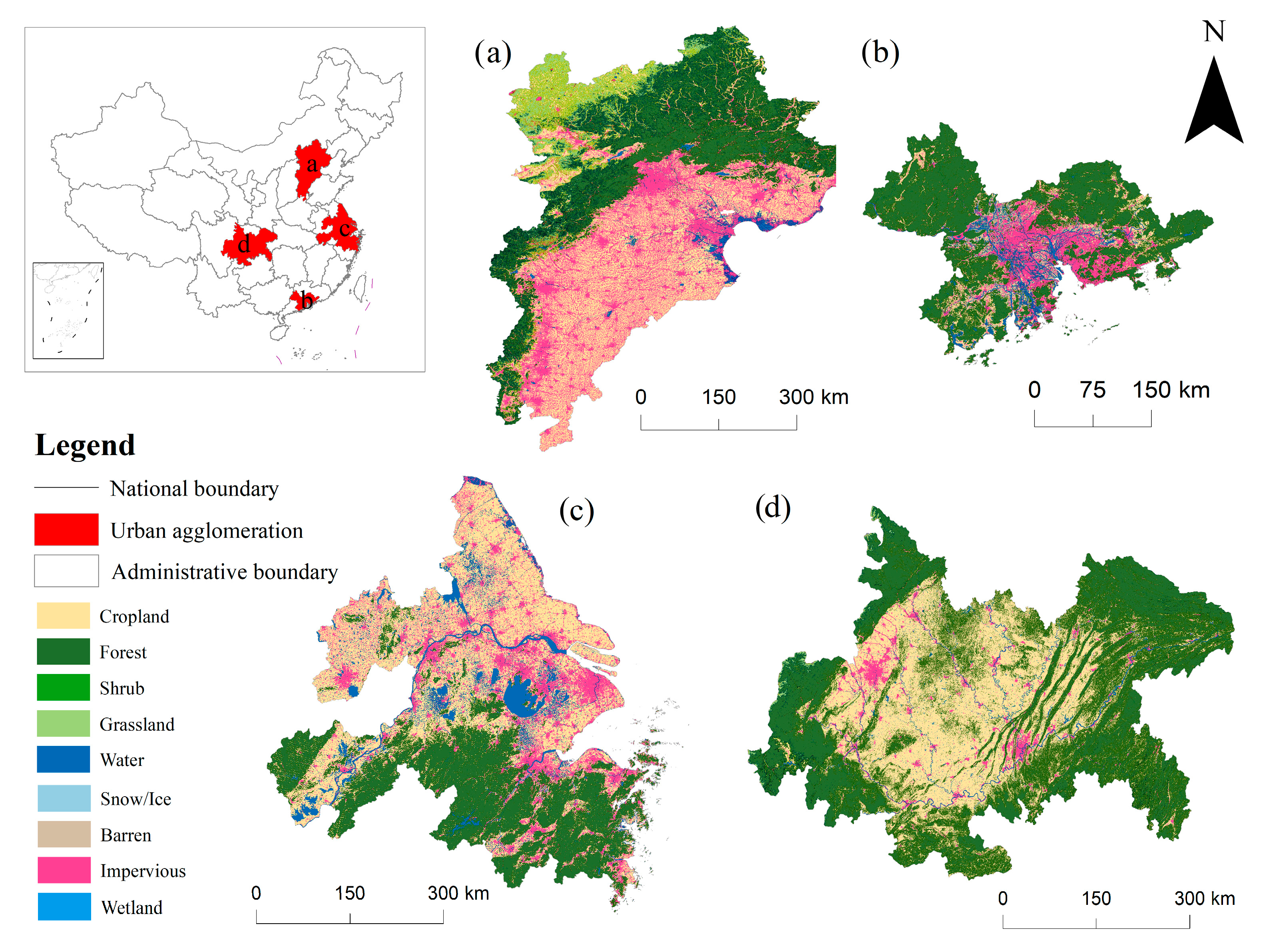
With the rapid economic development of China, the construction of many regions began to focus on the formation of urban agglomerations and megalopolises. The operational development between urban agglomerations will gradually replace the development of single cities. To date, a consensus on how to define an urban agglomeration has not been reached, although scholars agree that an urban agglomeration comprises multiple cities that are highly integrated. There is a clear difference between urban agglomerations and town agglomerations. Specifically, the cluster structure of an urban agglomeration requires a hierarchical structure with large, medium, and small-sized cities and towns, whereas a town agglomeration is essentially a cluster of small towns that does not necessarily have any meaningful hierarchical structure [21]. At present, China has formed four major urban agglomerations, namely the Beijing–Tianjin–Hebei urban agglomeration (BTH), the Pearl River Delta urban agglomeration (PRD), the Yangtze River Delta urban agglomeration (YRD), and the Chengdu–Chongqing urban agglomeration (CC). The geographical locations of the four core urban agglomerations are shown in Figure 1.

The BTH is China’s “Capital Economic Circle”. The PRD is developing together with the two special administrative regions of Hong Kong and Macao to build the Guangdong–Hong Kong–Macao Greater Bay Area. The YRD is an important intersection of the “Belt and Road” and the Yangtze River Economic Belt, and it plays a pivotal strategic role in the overall situation of China’s national modernization and opening up. The CC is an important platform for the development of Western China, a strategic support for the Yangtze River Economic Belt, and an important demonstration area for China to promote new urbanization.

2.2. Data Sources and Grid Design

2.2.1. Data Sources

The annual average PM_2.5 concentration grid of 0.01° × 0.01° (approximately 1 km × 1 km) from 1998 to 2021 was obtained from the Atmospheric Composition Analysis Organization (ACAG) (https://sites.wustl.edu/acag/datasets/surface-pm2-5/, accessed on 24 February 2024), which integrates data from remote sensing monitoring and site measurements. The annual precipitation data, the annual average temperature data, and the annual average wind speed data were derived from the National Earth System Science Data Center (http://www.geodata.cn/https://sites.wustl.edu/acag/datasets/surface-pm2-5/, accessed on 24 February 2024), which provided the annual precipitation data (2001–2020), the monthly average temperature data from 1901 to 2021, and the monthly average wind speed data (2001–2020) for China with a resolution of 1 km. The spatial resolution of the original data was 0.1°, and the precipitation unit, temperature unit, and wind speed unit were 0.1 mm, 0.1 °C, and m/s, respectively.

The land use data were derived from the national land cover dataset of Wuhan University, which has a spatial resolution of 30 m.

When processing PM_2.5 and meteorological data, regional statistical tools in ArcGIS can be used. The principle is to assign the pixel values of the pixels covered by a grid to the grid by summing them. Due to the time resolution of temperature and wind speed data being one month, we calculated the annual mean of the two types of data as the corresponding statistical data. The area indicator tool in ArcGIS was used to calculate the area of different land type attributes in each grid, and the statistical data were linked to the corresponding grid.

2.2.2. Grid Design

Compared with coarser atmospheric particles, PM_2.5 has a smaller particle size, meaning they can stay in the atmosphere for a long time and can be transported to distant locations. Currently, research on PM_2.5 is mostly based on cities and towns. Therefore, in order to better understand the relationship between different factors and the annual average PM_2.5 concentration in urban agglomerations, more scale information was needed. The division of grids at different scales can affect the results, so it was also necessary to conduct multiscale research. Because some researchers have applied a multiscale polygon grid-based analysis to the study of the urban heat island effect in the Beijing–Tianjin–Hebei region, these grid partitioning methods could be used for reference [18]. We set up a gradient of different sizes of grid for subsequent comparative analysis, taking 6, 9, 12, 15, and 18 km as the analysis scales. All of the grid sizes were designed to be an integer multiple of the pixel size of the thematic data (1 km for the PM_2.5 concentration, temperature, precipitation, and wind speed, and 30 m for land cover). This ensured that the data values of each pixel in the thematic data could be effectively linked to the grid. Figure 2 shows the annual precipitation in 2020 under different grid scales.

When conducting spatial regression analysis at different levels using panel data, all meteorological indicators were averaged within corresponding grid boundaries from 2010 to 2020. We used the regional statistical method to calculate the mean meteorological data for each grid. For the temperature and wind speed data, we calculated the annual average data through the monthly average data to ensure that the time scale of all data was the same.

3. Methodology

3.1. Spatiotemporal Pattern Analysis

Before conducting spatial econometric analysis to explore the impact of various factors on PM_2.5, it was necessary to verify whether the spatial distribution of PM_2.5 conformed to spatial autocorrelation. Only when it was determined that the spatial distribution of PM_2.5 had spatial autocorrelation characteristics could spatial measurements be carried out. Spatial statistical analysis is based on spatial connections, and it is divided into global autocorrelation and local autocorrelation. The estimation of global spatial autocorrelation describes the spatial features of geographical phenomena or attributes from an overall region, while local autocorrelation describes the spatial features of geographical phenomena or attributes from partial regions. In this paper, we chose Global Moran’s I to verify the spatial autocorrelation in PM_2.5. The calculation formula is:

$$I=\frac{n\sum _i\sum _j{W}_{ij}(x_i-\overline{x})(x_j-\overline{x})}{\sum _i\sum _j{W}_{ij}\sum _i{(x_i-\overline{x})}^2}=\frac{\sum _i\sum _j{W}_{ij}(x_i-\overline{x})(x_j-\overline{x})}{S^2\left(\sum _i\sum _j{W}_{ij}\right)}(i,j=\mathrm{1,2},\dots ,n)$$

(1)

where I is the value of Global Moran’s I; $S^2=\frac{1}{n}\sum _i{(x_i-\overline{x})}^2$; $\overline{x}=\frac{1}{n}\sum _i{x}_i$; $W_{ij}$ is the element in the spatial weight matrix that represents the impact between region $i$ and region $j$; $x_i$ and $x_j$ are the values of the PM_2.5 concentration in regions $i$ and $j$; $x_i$ is the mean value of the PM_2.5 concentration; and $n$ is the number of samples. In this study, the Queen adjacency matrix W was used as the spatial weight matrix.

$$\mathrm{W}=\left(\begin{array}{cccc}{W}_{11}& W_{12}& \dots & W_{1n}\\ W_{21}& W_{22}& \dots & W_{2n}\\ ⋮& ⋮& \ddots & ⋮\\ W_{n1}& W_{n2}& \dots & W_{nn}\end{array}\right)$$

(2)

$${\mathrm{W}}_{ij}=\left\{\begin{array}{c}1,\mathrm{g}\mathrm{r}\mathrm{i}\mathrm{d} \mathrm{i} \mathrm{i}\mathrm{s} \mathrm{a}\mathrm{d}\mathrm{j}\mathrm{a}\mathrm{c}\mathrm{e}\mathrm{n}\mathrm{t} \mathrm{t}\mathrm{o} \mathrm{g}\mathrm{r}\mathrm{i}\mathrm{d} \mathrm{j}\\ 0,\mathrm{g}\mathrm{r}\mathrm{i}\mathrm{d} \mathrm{i} \mathrm{i}\mathrm{s} \mathrm{n}\mathrm{o}\mathrm{t} \mathrm{a}\mathrm{d}\mathrm{j}\mathrm{a}\mathrm{c}\mathrm{e}\mathrm{n}\mathrm{t} \mathrm{t}\mathrm{o} \mathrm{g}\mathrm{r}\mathrm{i}\mathrm{d} \mathrm{j}\end{array}\right.$$

(3)

The range of Moran’s index lies between +1 and −1. When I is equal to +1, it suggests that the pattern observed is clustered spatially. On the other hand, when I is equal to −1, it suggests scattering or dispersion. An I value close or equal to zero points to the absence of autocorrelation.

3.2. Spatial Regression Model

Spatial regression analysis usually utilizes the linear regression model. Because PM_2.5 is likely to diffuse across regions, the OLS (Ordinary Least Square Model) estimations of the non-spatial panel model may be biased and inconsistent [22]. Thus, considering the evidence for spatial effects, the SDM (spatial Durbin model) was introduced in this research. Considering both endogenous spatial dependence in the dependent variable (Y) and exogenous spatial dependence in the explanatory variables (X), the SDM was written as:

$$\mathrm{Y}=\lambda WY+{\beta }_1{X}_1+{\beta }_{2}W{X}_1+{\beta }_3{X}_2+{\beta }_{4}W{X}_2+\dots +{\beta }_{13}{X}_7+{\beta }_{14}{X}_7+\epsilon ,\epsilon ~N(0,{\sigma }^2{I}_n)$$

(4)

where Y is a vector of the average annual PM_2.5 concentration; X is a matrix of the influencing factors of selection; W is the spatial weight matrix; WY is a vector of the spatial lag-dependent variable that denotes the endogenous interaction effects among Y; and WX is a vector of a spatial lag-independent variable that denotes the exogenous interaction effects among X. The coefficients ${\beta }_i$ ($i$ = 1, 2, …, 14) are the regression parameters, and λ is an additional parameter representing the spatial regression coefficient of WY. The term ε is a normally distributed disturbance term with a diagonal covariance matrix.

To determine the suitability of the SDM, several tests, such as the Hausman test, Lagrange multiplier test, robustness Lagrange multiplier test, likelihood ratio test, and Wald test, can be used. Firstly, the Hausman test was used on the constructed panel data, and it was found that the statistical values of both the spatially and temporally fixed models were significant at a 1% confidence level, indicating that the model had a fixed cross-section and a fixed time effect. Secondly, the necessity of extending the OLS model to spatial regression models was investigated using the Lagrangian multiplier (LM) test and the robust Lagrangian multiplier (RLM) test of SLM or SEM. There were two situations in the LM test in this article, and the following adjustments were made for the two different test results: (1) The test values of SLM-LM, SEM-LM, SEM-RLM, and SLM-RLM were all significant at a 1% confidence level, indicating that adding spatial dependencies in the spatial regression was necessary. Therefore, the SDM was used for regression. (2) In the LM test, there were test values that were not significant at a 1% confidence level, so we introduced spatial dependence items in spatial regression and used the spatial Durbin model (SDM) for regression. After regression, we performed the LR and WALD tests on SEM and SLM, and the results showed that the SDM cannot degenerate into SEM or SLM. This article adopted a more robust SDM with nested spatiotemporal bidirectional fixed effects for the analysis.

The spatial weight matrix used in the regression process was the same as the matrix used in the spatial spatiotemporal pattern analysis, which was an inverse distance matrix. Data for a time interval of 11 years were used to form panel data for regression. Spatial regression analysis was conducted using Elhorst’s Spatial Regression MATLAB 2022a toolbox [23]. In order to propose appropriate and feasible policy recommendations based on the fitting results, a normalization process was not applied in this study. Here, direct effects refer to the study of the impact of factors in the local grid on the PM_2.5 concentration, while spillover effects refer to the impact of all factors in the surrounding grid on the PM_2.5 concentration. Both direct and indirect effects can be calculated by the SDM. The total impact effect of the region was the sum of its direct effects and the indirect effects of the surrounding area.

Based on natural environmental changes and human activity, we classified the factors that affected the PM_2.5 concentration. In terms of natural environmental changes, precipitation (mm), temperature (°C), wind speed (m/s), forest (km²), and water area (km²) were selected as the independent variables. Cropland (km²) and impermeable surfaces (km²) were chosen as further independent variables. The PM_2.5 concentration was selected as the dependent variable. The independent variables were defined as follows:

• PRE: annual precipitation;
• TMP: annual average temperature;
• WND: annual average wind speed;
• CPL: the land use of cropland;
• FOREST: the land use of forests;
• WATER: the land use of water;
• IPS: the land use of impermeable surfaces.

4. Results and Analyses

4.1. Spatiotemporal Patterns of the PM_2.5 Concentration

The spatial patterns of the PM_2.5 concentration in the four core urban agglomerations in China from 2010 to 2020 are shown in Figure 3. The annual average PM_2.5 concentration in the BTH showed a trend of increasing first and then decreasing. The concentration in the southern region was significantly higher than that in the northern region. The areas with high concentrations were concentrated in the plains of the south. The annual average PM_2.5 concentration in the PRD appeared to have a declining trend and was relatively consistent in the whole region. The concentration in the Chengdu–Chongqing urban agglomeration showed a gradual decreasing trend from the center of the urban agglomeration outward, and the concentration in the western region was higher than that in the eastern region. The areas with high PM_2.5 concentrations were mainly distributed in the southern region of Sichuan, with Chongqing and Chengdu as the line of demarcation. In general, the concentration in the BTH was significantly higher than that of the other three urban clusters, with the PRD having the lowest concentration.

This paper used MATLAB tools to construct a spatial weight matrix and calculated Moran’s I based on the above Formula (1).

Table 1. The value of Moran’s I in the four core urban agglomerations in China in 2020.

Grid	BTH	PRD	YRD	CC
6 km	0.992 ***	0.944 ***	0.976 ***	0.970 ***
9 km	0.986 ***	0.897 ***	0.958 ***	0.957 ***
12 km	0.980 ***	0.858 ***	0.940 ***	0.943 ***
15 km	0.972 ***	0.791 ***	0.917 ***	0.926 ***
18 km	0.966 ***	0.719 ***	0.904 ***	0.903 ***

Notes: *, **, *** represent significance at the 10%, 5%, and 1% levels, respectively.

shows the value of Moran’s I in the four core urban agglomerations in 2020. According to the value of Moran’s I, the spatial distribution of PM_2.5 showed a significant spatial autocorrelation effect in the four major urban agglomerations, and all were positive.

4.2. Spatial Econometric Testing of the Influencing Factors of PM_2.5

4.2.1. Regression Model Identification

Considering the spatial autocorrelation of the PM_2.5 concentration described in Section 4.1, a spatial regression model was used to further explore the impact of different factors on the PM_2.5 concentration in different regions at different scales.

Table 2. Necessary tests for the experiments.

Name	Tests	Grid
		6 km	9 km	12 km	15 km	18 km
BHT	SLM-LM	13,696.97 ***	4398.65 ***	1921.41 ***	930.39 ***	568.19 ***
	SLM-RLM	37.16 **	17.04 ***	10.43 ***	5.77 **	3.94 **
	SEM-LM	167,629.41 ***	69,599.45 ***	36,460.26 ***	22,019.29 ***	14,062.00 ***
	SEM-RLM	153,969.60 ***	65,217.84 ***	34,549.28 ***	21,094.67 ***	13,497.75 ***
PRD	SLM-LM	397.82 ***	66.95 ***	7.89 **	23.10 ***	2.91 **
	SLM-RLM	0.38	0.05	0.02	0.24	0.05
	SEM-LM	32,409.20 ***	12,464.77 ***	5544.46 ***	2913.49 ***	1462.80 ***
	SEM-RLM	32,011.76 ***	12,397.86 ***	5536.59 ***	2890.63 ***	1461.93 ***
	SLM-LR	9045.75 ***	5829.31 ***	3076.38 ***	1884.30 ***	1073.15 ***
	SLM-WALD	13,374.82 ***	8000.14 ***	4701.32 ***	2365.86 ***	1553.49 ***
	SEM-LR	23,330.29 ***	11,935.92 ***	5968.71 ***	3304.76 ***	1864.52 ***
	SEM-WALD	1520.89 ***	561.71 ***	270.97 ***	153.28 ***	121.49 ***
YRD	SLM-LM	753.00 ***	222.23 ***	58.66 ***	36.85 ***	8.53 ***
	SLM-RLM	0.12	0.03	0.01	0.02	0.01
	SEM-LM	90,850.35 ***	56,947.38 ***	28,886.59 ***	15,586.31 ***	9970.70 ***
	SEM-RLM	90,097.48 ***	56,725.17 ***	28,827.95 ***	15,549.49 ***	9962.17 ***
	SLM-LR	6952.62 ***	3624.49 ***	1397.80 ***	334.66 ***	556.32 ***
	SLM-WALD	11,522.59 ***	5336.92 ***	3265.22 ***	1098.44 ***	1212.28 ***
	SEM-LR	35,987.88 ***	15,160.72 ***	8066.07 ***	3919.46 ***	3087.32 ***
	SEM-WALD	1150.83 ***	460.00 ***	325.07 ***	426.96 ***	157.50 ***
CC	SLM-LM	66,599.01 ***	14,155.22 ***	3195.68 ***	1401.74 ***	377.44 ***
	SLM-RLM	43.62 **	16.37 ***	5.99 **	4.25 ***	1.57
	SEM-LM	195,228.22 ***	81,183.65 ***	42,028.11 ***	25,138.77 ***	16,026.24 ***
	SEM-RLM	128,672.84 ***	67,044.80 ***	38,838.42 ***	23,741.27 ***	15,650.37 ***
	SLM-LR	-	-	-	-	519.88 ***
	SLM-WALD	-	-	-	-	898.87 ***
	SEM-LR	-	-	-	-	2417.39 ***
	SLM-WALD	-	-	-	-	114.48 ***

Notes: (1) *, **, *** represent significance at the 10%, 5%, and 1% levels, respectively; (2) spatial lag model (SLM), spatial error model (SEM), spatial Durbin model (SDM), Lagrangian multiplier (LM), robust Lagrangian multiplier (RLM), likelihood ratio (LR), Wald test (WALD).

shows the results of each test.

4.2.2. Regression Results

The results indicated that precipitation, temperature, cropland, and impermeable surfaces have a stable and significant negative impact on the PM_2.5 concentration in the BTH. In the PRD, precipitation has a stable and significant negative impact. In the YRD, precipitation and temperature have a stable and significant negative impact. In the CC, precipitation, temperature, cropland, forests, water bodies, and impermeable surfaces have a significant negative impact, while wind speed has a positive impact.

The data in

Table 3. Spatial regression estimation of the PM_2.5 concentration in the four urban agglomerations at different scales from 2010 to 2020.

Name	Variables	Grid
		6 km	9 km	12 km	15 km	18 km
BHT	PRE	−0.031 ***	−0.029 ***	−0.033 ***	−0.036 ***	−0.031 ***
	TMP	−5.646 ***	−6.758 ***	−7.404 ***	−9.902 ***	−8.951 ***
	WND	−0.188 ***	0.031	0.272	−0.541 *	0.513
	CPL	−0.031 ***	−0.024 ***	−0.022 ***	−0.016 **	−0.016 **
	FOREST	−0.046 ***	−0.017	−0.000	−0.007	0.028 ***
	WATER	0.012	−0.014	−0.063 ***	−0.038 **	−0.128 ***
	IPS	−0.115 ***	−0.088 ***	−0.096 ***	−0.068 ***	−0.060 ***
	W*PRE	0.005 ***	0.005 ***	0.006 ***	0.006 ***	0.005 ***
	W*TMP	0.964 ***	1.153 ***	1.250 ***	1.663 ***	1.532 ***
	W*WND	−0.003	−0.074 **	−0.149 ***	−0.036	−0.199 *
	W*CPL	0.012 ***	0.009 ***	0.008 ***	0.009 ***	0.009 ***
	W*FPREST	0.021 ***	0.013 ***	0.009 ***	0.010 ***	0.001
	W*WATER	−0.009 **	−0.012 ***	−0.006	0.001 ***	0.007
	W*IPS	0.026 ***	0.017 ***	0.017 ***	0.011 ***	0.012 ***
	W*(PM2.5)	0.165 ***	0.164 ***	0.163 ***	0.161 ***	0.163 ***
	R2	0.9993	0.9990	0.9987	0.9981	0.9802
PRD	PRE	0.000 **	0.001 ***	0.001 **	0.001	0.000
	TMP	−5.806 ***	−7.342 ***	−8.288 ***	−8.153 ***	−9.171 ***
	WND	0.021	−0.017	−0.104	−0.398 *	0.325
	CPL	0.010	−0.225 *	0.071	0.059	−0.022
	FOREST	0.073	−0.162	0.109	0.091	−0.012
	WATER	0.091	−0.137	0.138	0.099	0.001
	IPS	−0.079	−0.264 **	0.074	0.042	−0.034
	W*PRE	−0.000	−0.000 ***	−0.000 ***	−0.000 **	−0.000 **
	W*TMP	1.514 ***	1.710 ***	1.829 ***	1.710 ***	1.863 ***
	W*WND	−0.039 *	−0.043	0.003	0.106	0.087
	W*CPL	0.004	0.054	0.079 *	0.011	0.122 *
	W*FPREST	−0.013	0.038	0.067	−0.002	0.117 *
	W*WATER	0.010	0.049	0.076 *	0.014	0.132 **
	W*IPS	0.001	0.055	0.074 *	0.015	0.123 *
	W*(PM2.5)	0.138 ***	0.139 ***	0.140 ***	0.135 ***	0.130 ***
	R2	0.9966	0.9964	0.9961	0.9955	0.9946
YRD	PRE	−0.006 ***	−0.006 ***	−0.005 ***	−0.005 ***	−0.005 ***
	TMP	−5.873 ***	−6.610 ***	−7.059 ***	−1.576 ***	−6.422 ***
	WND	0.146 **	−0.165 *	−0.160	−0.363	−0.014
	CPL	0.281	−0.010	−0.217	0.187	0.216
	FOREST	0.303	0.002	−0.211	0.217	0.234
	WATER	0.337	0.063	−0.162	0.157	0.221
	IPS	0.282	−0.020	−0.231	0.147	0.188
	W*PRE	0.001 ***	0.001 ***	0.001 ***	0.001 ***	0.001 ***
	W*TMP	1.200 ***	1.317 ***	1.468 **	0.879 ***	1.395 ***
	W*WND	−0.033 **	0.054 *	0.118 ***	0.282 ***	0.331 ***
	W*CPL	0.182 **	0.219 ***	0.299 ***	0.151 *	0.153 **
	W*FPREST	0.195 ***	0.230 ***	0.308 ***	0.154 *	0.159 **
	W*WATER	0.172 **	0.202 **	0.283 ***	0.151 *	0.148 *
	W*IPS	0.179 **	0.217 ***	0.296 ***	0.155 **	0.152 *
	W*(PM2.5)	0.152 ***	0.149 ***	0.147 ***	0.139 ***	0.134 ***
	R2	0.9963	0.9950	0.9941	0.9916	0.9904
CC	PRE	−0.018 ***	−0.019 ***	−0.020 ***	−0.017 ***	−0.014 ***
	TMP	−0.665 ***	−1.909 ***	−3.191 ***	−4.369 ***	−6.133 ***
	WND	0.735 ***	0.523 ***	0.377 ***	0.388 *	0.446 *
	CPL	−0.234 ***	−0.264 ***	−0.184 ***	−0.181 ***	−0.267 ***
	FOREST	−0.229 ***	−0.263 ***	−0.182 ***	−0.176 ***	−0.265 ***
	WATER	−0.209 ***	−0.295 ***	−0.169 **	−0.207 ***	−0.324 ***
	IPS	−0.217 ***	−0.266 ***	−0.202 ***	−0.210 ***	−0.297 ***
	W*PRE	0.003 ***	0.003 ***	0.003 ***	0.003 ***	0.002 ***
	W*TMP	0.132 ***	0.337 ***	0.547 ***	0.729 ***	1.011 ***
	W*WND	−0.227 ***	−0.216 ***	−0.273 ***	−0.322 ***	−0.342 ***
	W*CPL	0.061 ***	0.064 ***	0.037 ***	0.047 ***	0.057 ***
	W*FPREST	0.062 ***	0.065 ***	0.038 ***	0.048 ***	0.058 ***
	W*WATER	0.115 ***	0.101 ***	0.083 ***	0.091 ***	0.085 ***
	W*IPS	0.038 ***	0.053 ***	0.032 ***	0.045 ***	0.057 ***
	W*(PM2.5)	0.159 ***	0.159 ***	0.157 ***	0.155 ***	0.157 ***
	R2	0.9978	0.9973	0.9962	0.9947	0.9951

Notes: (1) *, **, *** represent significance at the 10%, 5%, and 1% levels, respectively; (2) variable names are explained in Section 3.2; (3) W*PRE was the spatial lagged terms of the PRE. The same convention was used for all other variables.

showed that the estimates of W*(PM_2.5) were significant at the 99th percentile confidence interval in the SDM models, indicating that for BTH, the PM_2.5 concentrations of the grid within the agglomeration increased by more than 0.16 μg/m³ for every 1 μg/m³ increase in the average PM_2.5 of neighboring grids. Similarly, in the PRD, YRD, and CC, the value was estimated to be 0.10 μg/m³, 0.13 μg/m³, and 0.15 μg/m³, respectively. Considering that the influencing mechanisms of different indicators were complex and varied at different temporal scales (e.g., day, month, and year) and spatial scales (e.g., grid, city, region, and country), not every indicator passed the significance test in the models.

In order to better study the marginal effects of various indicators selected in this article on the PM_2.5 concentration, the spatial effects were separated, and the spatial interaction effects were tested with consideration of two aspects: direct effects and spillover effects.

Table 4. Direct effects, spillover effects, and total effects of different factors on PM_2.5 in the Beijing–Tianjin–Hebei urban agglomeration (BTH).

Grid	Impact	Variable
		PRE	TMP	WND	CPL	FOREST	WATER	IPS
6 km (N = 6340)	Direct	−0.030 ***	−5.392 ***	−0.440 ***	0.017	0.052 ***	−0.040	−0.063 ***
	Spillover	−0.000 ***	−0.214 ***	0.207 ***	−0.040 ***	−0.083 ***	0.043 **	−0.044 ***
	Total	−0.030 ***	−5.606 ***	−0.232 ***	−0.023 **	−0.031 **	0.003	−0.107 ***
9 km (N = 2485)	Direct	−0.028 ***	−6.470 ***	−0.404 **	−0.010	0.051 ***	−0.102 ***	−0.071 ***
	Spillover	−0.000 *	−0.235 ***	0.349 ***	−0.027 ***	−0.055 ***	0.072 ***	−0.014
	Total	−0.029 ***	−6.705 ***	−0.054	−0.017 **	−0.004	−0.030 *	−0.084 ***
12 km (N = 1354)	Direct	−0.033 ***	−7.185 ***	−0.237	0.001	0.042 ***	−0.143 ***	−0.091 ***
	Spillover	−0.001 ***	−0.162 ***	0.386 ***	−0.017 ***	−0.032 ***	0.061 ***	−0.004
	Total	−0.033 ***	−7.347 ***	0.148	−0.016 **	0.011	−0.083 ***	−0.095 ***
15 km (N = 849)	Direct	−0.035 ***	−9.583 ***	−1.082 ***	0.010	0.032 ***	−0.060 *	−0.067 ***
	Spillover	−0.001 ***	−0.228 *	0.383 *	−0.019 ***	−0.028 ***	0.016	−0.001
	Total	−0.035 ***	−9.810 ***	−0.698 **	−0.009	0.004	−0.044 **	−0.067 ***
18 km (N = 565)	Direct	−0.030 ***	−8.584 ***	−0.065	0.014 *	0.055 ***	−0.197 ***	−0.048 ***
	Spillover	−0.001 **	−0.280 ***	0.439 ***	−0.023 ***	−0.021 ***	0.052 **	−0.009
	Total	−0.031 ***	−8.864 ***	0.374 ***	−0.009	0.035 ***	−0.144 ***	−0.058 ***

Notes: *, **, *** represent significance at the 10%, 5%, and 1% levels, respectively.

presents the direct and spillover effects of various influencing factors on the BTH,

Table 5. Direct effects, spillover effects, and total effects of different factors on PM_2.5 in the Pearl River urban agglomeration (PRD).

Grid	Impact	Variable
		PRE	TMP	WND	CPL	FOREST	WATER	IPS
6 km (N = 1210)	Direct	0.001 ***	−4.508 ***	−0.041	0.018	0.065	0.130	−0.098
	Spillover	−0.000 ***	−0.468 ***	−0.024 ***	0.003	0.003	−0.014	0.007
	Total	0.000 ***	−4.976 ***	−0.017	0.015	0.068	0.116	−0.091
9 km (N = 499)	Direct	0.001 ***	−6.091 ***	−0.101	−0.189	−0.139	−0.087	−0.237
	Spillover	0.000	−0.447 ***	0.030	−0.015	−0.010	−0.019	−0.012
	Total	0.001 ***	−6.538 ***	−0.071	−0.204	−0.149	−0.107	−0.249 *
12 km (N = 251)	Direct	0.001 *	−7.062 ***	−0.127	0.225	0.252	0.305 *	0.220
	Spillover	0.000 *	−0.451 ***	0.007	−0.060 **	−0.055 *	−0.064 **	−0.057 **
	Total	0.001 *	−7.513 ***	−0.120	0.166	0.197	0.241 *	0.163
15 km (N = 152)	Direct	0.000	−7.169 ***	−0.322	0.085	0.104	0.138	0.072
	Spillover	0.000 **	−0.275 ***	−0.023	−0.008	−0.004	−0.012	−0.009
	Total	0.000	−7.444 ***	−0.346	0.077	0.100	0.126	0.063
18 km (N = 96)	Direct	−0.000 ***	−8.168 ***	0.528	0.158	0.164	0.200	0.145
	Spillover	0.000 **	−0.227 ***	−0.046	−0.041	−0.040	−0.046 *	−0.041
	Total	−0.000	−8.395 ***	0.482	0.117	0.124	0.155	0.104

Notes: *, **, *** represent significance at the 10%, 5%, and 1% levels, respectively.

the PRD,

Table 6. Direct effects, spillover effects, and total effects of different factors on PM_2.5 in the Yangtze River urban agglomeration (YRD).

Grid	Impact	Variable
		PRE	TMP	WND	CPL	FOREST	WATER	IPS
6 km (N = 4663)	Direct	−0.006 ***	−5.018 ***	0.116 *	0.896 ***	0.963 ***	0.947 ***	0.889 ***
	Spillover	−0.000 ***	−0.488 ***	0.017	−0.359 ***	−0.385 ***	−0.356 ***	−0.354 ***
	Total	−0.006 ***	−5.506 ***	0.132 **	0.537 *	0.578 **	0.590 **	0.535 *
9 km (N = 1942)	Direct	−0.005 ***	−5.779 ***	−0.090	0.541 *	0.586 *	0.598 ***	0.523 *
	Spillover	−0.000 ***	−0.441 ***	−0.039	−0.292 ***	−0.309 ***	−0.283 ***	−0.287 ***
	Total	−0.005 ***	−6.220 ***	−0.129	0.250	0.277	0.314	0.236
12 km (N = 1034)	Direct	−0.005 ***	−6.061 ***	0.060	0.406	0.435	0.441 *	0.381
	Spillover	−0.000 ***	−0.498 ***	−0.107 **	−0.309 ***	−0.320 ***	−0.299 ***	−0.303 ***
	Total	−0.005 ***	−6.559 ***	0.048	0.097	0.114	0.142	0.078
15 km (N = 600)	Direct	−0.004 ***	−0.357 **	0.071	0.510 *	0.553 **	0.472 *	0.467 *
	Spillover	−0.000 ***	−0.459 ***	−0.161 ***	−0.121 **	−0.126 **	−0.118 **	−0.120 **
	Total	−0.005 ***	−0.817 ***	−0.090	0.389 *	0.427 *	0.354	0.348
18 km (N = 403)	Direct	−0.005 ***	−5.532 ***	0.526	0.525 **	0.556 **	0.522 ***	0.488 *
	Spillover	−0.000 ***	−0.278 ***	−0.169 ***	−0.097 **	−0.101 **	−0.094 **	−0.094 **
	Total	−0.005 ***	−5.810 ***	0.356	0.428 *	0.455 *	0.427 *	0.394 *

Notes: *, **, *** represent significance at the 10%, 5%, and 1% levels, respectively.

the YRD, and

Table 7. Direct effects, spillover effects, and total effects of different factors on PM_2.5 in the Chengdu–Chongqing urban agglomeration (CC).

Grid	Impact	Variable
		PRE	TMP	WND	CPL	FOREST	WATER	IPS
6 km (N = 6353)	Direct	−0.018 ***	−0.521 ***	0.132 **	−0.104 ***	−0.088 **	0.235 ***	−0.199 ***
	Spillover	−0.000 ***	−0.112 ***	0.474 ***	−0.102 ***	−0.111 ***	−0.349 ***	−0.015
	Total	−0.018 ***	−0.633 ***	0.606 ***	−0.206 ***	−0.199 ***	−0.114 **	−0.214 ***
9 km (N = 2739)	Direct	−0.018 ***	−1.779 ***	0.007	−0.178 ***	−0.172 ***	−0.085	−0.226 ***
	Spillover	−0.000 ***	−0.089 ***	0.357 ***	−0.060 ***	−0.063 ***	−0.144 ***	−0.028 ***
	Total	−0.018 ***	−1.868 ***	0.364 ***	−0.238 ***	−0.235 ***	−0.229 ***	−0.254 ***
12 km (N = 1478)	Direct	−0.019 ***	−3.043 ***	−0.318 **	−0.155 ***	−0.149 ***	0.017	−0.202 ***
	Spillover	−0.000 ***	−0.099 ***	0.448 ***	−0.019 ***	−0.021 ***	−0.119 ***	−0.001
	Total	−0.020 ***	−3.142 ***	0.130	−0.174 ***	−0.170 ***	−0.102 *	−0.203 ***
15 km (N = 927)	Direct	−0.017 ***	−4.197 ***	−0.435 *	−0.120 ***	−0.109 ***	−0.023	−0.169 ***
	Spillover	−0.000 ***	−0.100 **	0.515 ***	−0.038 ***	−0.041 ***	−0.116 ***	−0.025 ***
	Total	−0.017 ***	−4.298 ***	0.080	−0.158 ***	−0.150 ***	−0.139 **	−0.194 ***
18 km (N = 623)	Direct	−0.014 ***	−5.985 ***	−0.463	−0.217 ***	−0.211 ***	−0.212 ***	−0.263 ***
	Spillover	−0.000 ***	−0.101 *	0.579 ***	−0.032 ***	−0.035 ***	−0.071 **	−0.022 ***
	Total	−0.014 ***	−6.086 ***	0.116	−0.249 ***	−0.246 ***	−0.283 ***	−0.286 ***

Notes: *, **, *** represent significance at the 10%, 5%, and 1% levels, respectively.

the CC.

The results in Table 4 showed that the estimated direct and spillover effects of PRE and TMP on PM_2.5 emissions were highly significant at the 1% level in the BTH at full scale, and their signs were negative, as expected. The effect of a 1 mm increase in annual precipitation will thus lead to a more than 0.03 μg/m³ decrease in PM_2.5 emissions, with other variables held constant. Similarly, for average annual temperature, the value was estimated to be 5.39 μg/m³. The spillover effect of precipitation was significant and the value was 0, indicating that the impact of annual precipitation in surrounding areas on the annual PM_2.5 can be ignored. Moreover, for temperature, the adjacent area had an average annual temperature increase of 1 °C, and the PM_2.5 in the study area decreased by about 0.20 μg/m³. In contrast, the direct impact of the average annual wind speed on PM_2.5 was negative and significant. Only under a grid of 12 km was the direct effect of this factor found not to be significant. The spillover effect was significantly positively correlated with PM_2.5, suggesting that the ambient wind speed conditions play a crucial role in the local PM_2.5. Interestingly, the direct effects of cropland were not significant under most scales, while forests were significantly positive. The spillover effect of both factors was significantly negative. The direct and spillover effects of water on the BTH varied between significant and insignificant. The direct effects of impermeable surfaces were significantly negative, while the spillover effect was not significant. This means that increasing the impermeable areas in adjacent areas does not have a significant impact on the local PM_2.5.

The direct effect of precipitation was significantly positive in the PRD, but its spillover effect was not significant and tended towards zero. This means that the influence of precipitation in the surrounding areas on the local PM_2.5 can be ignored. There was a negative correlation between the local temperature and PM_2.5, while the correlation between the temperature in neighboring areas and local PM_2.5 was not significant. The influence of wind speed on PM_2.5 in the PRD can be ignored. The direct effect of cropland and forests on PM_2.5 in the PRD was significantly negative, while the spillover effect was not significant. The impact of water bodies and impermeable surfaces on PM_2.5 in the PRD was not significant.

The direct and spillover effects of precipitation in the YRD were significantly negative, with small fluctuations in the direct effects and negligible spillover effects. The direct and spillover effects of the temperature were also significantly negative. It is worth noting that under a 15 km grid, the direct and spillover effects of temperature were similar in size. The adjustment effect of land use factors was similar, with local factors positively correlated with the local PM_2.5, while neighboring factors negatively correlated with the local PM_2.5, and the direct effect was about twice as large as the spillover effect.

The precipitation of the CC was negatively correlated with PM_2.5, and the spillover effect can be ignored. Temperature was negatively correlated with PM_2.5, and as the research scale increased, the direct influence of temperature increased. The wind speed spillover effect was larger, but contrary to expectations, an increase in wind speed in adjacent areas will actually lead to an increase in local PM_2.5. The direct effect and spillover effect of the two green indicators for cropland and forest were similar and showed a significant negative correlation with PM_2.5. The magnitude of the direct effect and spillover effect was also similar. The indirect impact of water bodies was significantly negative, and their direct impact was not significant at some scales. Furthermore, the direct effect under the conditions of the smallest and largest research units showed the opposite. It is worth noting that there was a negative relationship between impermeable surfaces and PM_2.5.

5. Discussion

5.1. The Relationship between Impacts and Scales

In previous studies that used counties or cities as research units, there was a clear demarcation between data from neighboring counties or cities. The significance of the different grid scales in this research was to reduce the deviation of data between each county or city and to better align the research results with the actual transmission characteristics of PM_2.5. The results showed that as the research scale increased, spatial Moran’s index I of the average annual PM_2.5 and the fitting index R² of the SDM gradually decreased. This was similar to the finding of Wang et al., where the model fitting results had gradient effects at different research scales, consistent with the first law of geography [18]. For the YRD, as the research scale increased, the importance of the direct and spillover effects of land use type factors decreased. This means that as the scale of research increases, the influence of land use type on PM_2.5 becomes correspondingly weaker. For the PRD, the direct and spillover effects of several factors were not significant. However, at a grid scale of 6 km, the fitting effect was better than at other scales, indicating that for the PRD, reducing the research scale and increasing the number of samples may make the adjustment effect more obvious.

5.2. Potential Causes of the Direct and Spillover Effects

5.2.1. Precipitation

Under different humidity conditions, the influence of precipitation on the PM_2.5 concentration was inconsistent. In the drier BTH, precipitation helps wash fine particulate matter out of the air, so the direct effect of precipitation is significantly negative [24]. Research has shown that under clean conditions, different amounts of precipitation can lead to an increase in PM_2.5. Compared to other urban agglomerations, PM_2.5 in the PRD was naturally lower and the urban agglomeration structure is closer to the coast, resulting in higher humidity. This led to a positive correlation between precipitation and PM_2.5 [24,25]. However, for the YRD, its direct effect was significantly negative due to the large sample size and the fact that multiple cities are not located near the coast. The direct and indirect effects were small, such that precipitation in the YRD only had a minor influence. In the CC, the concentration is influenced by the unique terrain and climatic conditions, where the surface wind speed is low, the proportion of calm is high, the air humidity is high, and the diffusion of atmospheric pollutants is slow. The decrease in PM_2.5 may have been related to frequent precipitation in the subtropical monsoon climate [26].

5.2.2. Temperature

The higher the temperature, the faster the rate of diffusion of a gas, the greater the temperature difference in the vertical direction, the stronger the upward movement, and the easier convection occurs, accelerating the transport and dilution of particles. High temperatures may lead to intense vertical dispersion of pollutants, leading to both direct and indirect effects of temperature that were negative in the BTH [27]. Due to the subtropical monsoon climate, temperature changes in the PRD were found to be much lower than in high-latitude areas, with an average annual temperature of about 22 °C. The higher the temperature, the stronger the air convection at the bottom, which promotes the upward transport of certain substances and thus reduces particulate matter (PM_2.5) [4]. Under high temperatures and strong solar radiation, the degradation rate of PM_2.5 is usually faster in the YRD [28]. For the Chengdu–Chongqing urban agglomeration, the average annual temperature is about 15 °C, and high-temperature weather favors the formation of convective weather. This is one of the reasons for the increased diffusion of pollutants.

5.2.3. Wind Speed

As the research scale increased, the direct benefits of wind speed in the BTH were shown to be not significant, while the spillover benefits of wind speed always showed a strong positive correlation. The impact of increasing wind speed in different directions on PM_2.5 was also different [29]; it can be inferred that the low-wind-speed conditions in the BTH do not support the diffusion of PM_2.5 [30]. A poor correlation between the PM_2.5 concentration and wind speed was found in the PRD and YRD. In these two urban agglomerations, the influence of wind speed on PM_2.5 was more complex [31]. Conditions in the CC are more conducive to the transmission of pollutants due to the flat terrain. Therefore, some of the pollutants generated in the northern and central regions of China are transported to the central region by the wind, which partly causes the increase in PM_2.5 in the region [32].

5.2.4. Cropland

The BTH is located in the northern part of China and the climate is dry. Soil wind erosion, farmland dust, and post-harvest biomass burning in fields have led to an increase in the PM_2.5 concentration due to the expansion of farmland area in the BTH [33]. As a vegetation type, arable land reduces sand and dust pollution through root anchoring and wind protection, thereby reducing the PM_2.5 concentration [34]. Fortunately, the total impact of agricultural land in the BTH showed a significant negative effect. In the YRD, although burning straw has been strictly prohibited, air pollution caused by biomass burning is still one of the main reasons for the increase in the PM_2.5 concentration [35]. However, as a type of vegetation, cropland reduces PM_2.5 concentrations through sedimentation. The CC has a subtropical humid monsoon climate. It is warm and humid all year round, with unique agricultural conditions and a large yield of green agricultural products [36]. Therefore, the direct and indirect effects of cropland in the region are significantly negative.

5.2.5. Forests

For the BTH, there has been a significant positive relationship between the direct impact of forests and PM_2.5 over a long period of time. This is due to the fact that particulate matter is more suspended at lower altitudes [37], and due to the low forest cover, the presence of forests does not lead to a reduction in PM_2.5. On the other hand, the spillover effect is that forests can prevent an influx of PM_2.5 by reducing wind speed or changing wind direction, resulting in the dry deposition of pollutant particles [38]. Although forests density is low, it has some indirect effects on the local PM_2.5. In the PRD, forests have a significant negative impact on the PM_2.5 concentration. The main component of fine particulate matter is metal elements. When humidity or rainfall increases, fine particles enter the soil through moisture deposition in forests. Under humid conditions, they promote the absorption of metal components by the soil and thus reduce the concentration of PM_2.5. Wildlife plays an important role in influencing PM_2.5 exposure in the YRD region. Biomass burning in forests and smoke emitted by wildlife contribute to the increase in PM_2.5 caused by forests [39]. Similar to cropland, forests, as a vegetation type, reduce the concentration of PM_2.5 in the air through sedimentation and adsorption in the climate of the CC [40].

5.2.6. Water Bodies

In the BTH, the impact of water on PM_2.5 has two outcomes. On the one hand, the evaporation of water increases the humidity in local areas, which is not conducive to the deliquescence and diffusion of PM_2.5, and this explains why the direct effect of water bodies in the region is positive. On the other hand, water has the ability to absorb atmospheric pollutants, leading to a negative indirect effect [10]. The YRD is located on the lower reaches of the Yangtze River and has well-developed waterways. Low-quality fuel is one of the sources of PM_2.5 [41]. Multiple studies have also shown that PM_2.5 concentrations are higher near bodies of water than in areas without bodies of water. From a landscape perspective, the “source” effect of bodies of water becomes apparent as the surface area increases. Water bodies promote the hygroscopic growth of PM_2.5, which leads to an increase in PM_2.5 near the water body [35]. This is one of the reasons why the direct effect of water bodies in the CC is positive, while the spillover effect is negative.

5.2.7. Impermeable Surfaces

A more compact urban layout often reduces the urban traffic volume, improves industrial efficiency, reduces pollutant emissions, and thus reduces PM_2.5 [42]. The expansion speed of BTH and CC has gradually slowed down in the past decade, with more emphasis on adapting the urban structure. Therefore, it is reasonable that an increase in impermeable surfaces will lead to significant negative direct and indirect impacts. The YRD has always had a high number of areas with high population mobility. The continuous urban expansion and the increase in road network density contribute to the increase in PM_2.5 [3]. At the same time, the increase in household pollution emissions caused by the population gathering and mobility caused by urban expansion is also one of the reasons for the significant positive total effect [43].

5.3. The Impacts of Factors Vary with Scales

A significant gradient effect was found for various factors in different urban agglomerations at different research scales. The impact of precipitation on PM_2.5 in the PRD showed an inverted U-shape with the change in research scale, while in other urban agglomerations, the influence of precipitation on PM_2.5 remained essentially unchanged (Figure 4a). The PRD should consider air quality after heavy rainfall. The influence of temperature on the BTH and CC increased, while the influence on the YRD decreased, as the research scale increased. The change in impact on the PRD was relatively small (Figure 4b). The impact of wind speed on inland urban agglomerations was more significant, and the influence of wind speed gradually increased (Figure 4c). This may have been because, as the research scale increased, the change in wind speed was more obvious, resulting in better dilution of PM_2.5. However, if inland urban agglomerations are affected by typhoons, outdoor activities should be reduced as much as possible in the short period after the typhoon weather ends.

Compared with other land use type factors, the influence of water bodies on the BTH changed relatively clearly with the increasing research scale, showing an inverted U-shape (Figure 4f), which may have been related to the design of urban water networks. The impact of cropland and forests on the PRD was more significant compared to other land use type factors, but the influence of the changes was not obvious (Figure 4d,e). This means that reclaiming more cropland and increasing forest cover may not have an optimal impact on PM_2.5. What is more important is the sensible consideration of the spatial arrangement of different types of vegetation. In the YRD, the influence of land use type factors on PM_2.5 changed gradually with the change in the research scale, and the amplitude of the change was obvious, showing a clear U-shape. Since the direct effect of each factor was positive, it can be roughly inferred that the effect of each influencing factor reached the minimum in the range of about 15 km. Therefore, the planning area of approximately 15 km must be taken into account when adjusting the city layout. As with the BTH, which is also an inland urban agglomeration, the effects of water bodies on the CC varied more with the scope of the research than with other factors. The design of water networks and artificial lakes in parks in inland urban agglomerations is very important. The spillover effect of land use factors on the BTH and CC showed a flat linear pattern with the increase in the research scale, which means that the impact of land use factors on the BTH and CC will not change significantly with the increase in the research scale.

The results (Section 4.2.2) indicate that the SDM model captures the nonlinear contribution rates of various influencing factors to the PM_2.5 concentration at different grid scales. Understanding these impact mechanisms may be of great significance for balancing urban planning, artificial weather assistance, and the joint prevention and control of PM_2.5 among urban agglomerations. For instance, in previous studies, there was a negative correlation between forest coverage and PM_2.5 concentration. However, this study found that the direct impact of forest coverage in urban agglomerations such as the BTH and the YRD would lead to an increase in PM_2.5 concentration. In other aspects, this study captured the influence curves of the direct effects of various influencing factors (Figure 4). After comprehensive consideration, it was found that the impact of various factors on BTH at the 18 km grid scale were generally optimal in reducing the PM_2.5 concentration. The impact on coastal urban clusters was good at a 6 km grid scale. The impact on the CC was optimal at the grid scales of 12 km and 15 km.

5.4. Relevant Policy Recommendations and Limitations

Due to the different geographical locations and natural climate conditions of major urban agglomerations, as well as the different development methods and directions of each urban agglomeration, policies for collaborative control of PM_2.5 should be formulated based on the inherent conditions of different urban agglomerations. Firstly, in response to the significant alleviation of PM_2.5 caused by precipitation in the BTH, relevant departments could consider increasing the frequency of artificial precipitation enhancement. Secondly, carbon emissions are one of the main causes of global warming, and the significant increase in population and the large amount of greenhouse gases generated by human activities after the Industrial Revolution are the main causes of global warming [44]. Due to the accumulation of PM_2.5 caused by the rise in temperature, relevant departments at all levels should diligently implement the “dual-carbon” policy. Thirdly, although the contribution of agricultural modernization to air pollution in agricultural production is negligible compared to industrial production, it is still necessary to encourage farmers to use agricultural machinery judiciously, and to use gentle soil cultivation methods such as covering with straw and digging less to extract less soil in suitable areas [45]. Fourthly, the ship emission control policy should continue to be implemented [21] in the PRD and YRD, and more air pollution-related policies should be added to the new fuel policy to reduce PM_2.5 generated by water navigation. Finally, the minimum scale in this article was equivalent to the district- or township-level scale, and the maximum scale was equivalent to the city level or half the actual scale. Villagers at the community level should be encouraged to actively report and expose straw-burning behavior or polluting companies and thereby address PM_2.5 issues on a small scale. All municipal units should be encouraged to jointly develop ideas and find ways to strengthen the management of relevant units at all levels of government and also take effective measures on a large scale.

From a research-scale perspective, we still discovered several interesting phenomena. As the grid scale increases, the spatial autocorrelation of PM_2.5 gradually weakens and shows a gradient decreasing trend. However, from the perspective of the total effects of various factors, it seems that their impact on PM_2.5 does not increase with the increase in grid scale. For example, in BTH, land use factors showed the highest impact at an 18 km grid scale, while meteorological factors showed the highest impact at a 6 km grid scale. This means that the optimal impact scale of meteorological factors and land use factors is inconsistent. The SDM can be used as a prediction model as follows: consider the land use plan and climate conditions for a given area, involving, for instance, (1) developing a reasonable watering plan for sprinkler trucks, (2) improving the distribution of vegetable gardens in rural homesteads, (3) the reasonable planning of urban water networks, (4) expanding urban roads. However, after implementing the plan, it is necessary to use the SDM for fitting predictions and continuously optimize policy guidelines to alleviate PM_2.5. It should also be clarified that the grid scale that can maximize the impact on PM_2.5 mentioned in this article may not be the optimal scale for prediction, and more detailed grid division is needed in different regions.

This study found that precipitation and temperature have a significant impact on the PM_2.5 concentration in different urban agglomerations, but the impact of wind speed on coastal urban agglomerations is not very significant. This may be because the impact of wind on PM_2.5 is relatively complex, and a more detailed small-scale analysis should be carried out based on wind direction and other factors.

6. Conclusions

This study analyzed the spatial dependence of the average annual PM_2.5 in the four core urban agglomerations in China and quantified the direct and spillover effects of various meteorological factors and land use types in neighboring cities, which complemented the analysis of the influence of various factors on PM_2.5 under different scales. The results are as follows.

• The average annual PM_2.5 concentration in the four core urban agglomerations in China generally showed a downward trend and was lower in the PRD than in the other three urban agglomerations.
• The PM_2.5 concentrations showed obvious spatial autocorrelation. After the LM test, Wald test, and LR test, we found that spatial econometric models can be introduced when studying the spatial distribution and influencing factors of PM_2.5.
• Overall, in the direct effects, meteorological factors were found to have a significant negative impact on the BTH, significantly positive effect on forests, and significantly negative effect on water bodies and impermeable surfaces. In the PRD, the influence of temperature was significantly negative. In the YRD, the impact of precipitation and temperature was significantly negative, while the impact on land use factors was significantly positive. The impact of precipitation, temperature, cropland, forests, and impermeable surfaces in the CC was significantly negative.
• On the whole, in the BTH, the indirect effects of precipitation, temperature, cropland, forests, and impermeable surfaces were found to be significantly negative, while their effects on wind speed and water bodies were significantly positive. The impact of temperature in the PRD was significantly negative. The impact of precipitation, temperature, and land use factors in the YRD was significantly negative. In the CC, the impact of precipitation, temperature, and land use factors was significantly negative, while the impact of wind speed was significantly positive.
• The influence of wind speed on coastal urban clusters was not significant among the meteorological factors, but it had a significant impact on inland urban clusters. The direct effect of land use factors showed a significant U-shaped change with the change in research scale in the YRD, and the direct effect was more than twice as large as the spillover effect.
• Among the land use factors, human factors (impermeable surfaces) in inland urban agglomerations were found to have a greater influence than natural factors in inland urban agglomerations, while natural factors (forests) were found to have a greater influence in coastal urban agglomerations.
• Targeted prevention and control measures should be utilized according to different regions and scales in different urban agglomerations.

References

- Fang, C.; Yu, D. Urban agglomeration: An evolving concept of an emerging phenomenon. Landsc. Urban Plan. 2017, 162, 126–136. [Google Scholar] [CrossRef]
- Geng, G.; Zheng, Y.; Zhang, Q.; Xue, T.; Zhao, H.; Tong, D.; Zheng, B.; Li, M.; Liu, F.; Hong, C.; et al. Drivers of (PM2.5) air pollution deaths in China 2002–2017. Nat. Geosci. 2021, 14, 645–650. [Google Scholar] [CrossRef]
- Chen, Z.; Chen, D.; Zhao, C.; Kwan, M.P.; Cai, J.; Zhuang, Y.; Zhao, B.; Wang, X.; Chen, B.; Yang, J.; et al. Influence of meteorological conditions on PM (2.5) concentrations across China: A review of methodology and mechanism. Environ. Int. 2020, 139, 105558. [Google Scholar] [CrossRef] [PubMed]
- Li, X.; Feng, Y.J.; Liang, H.Y. The Impact of Meteorological Factors on (PM2.5) Variations in Hong Kong. In IOP Conference Series: Earth and Environmental Science; IOP Publishing: Bristol, UK, 2017; Volume 78. [Google Scholar]
- Wu, W.; Zhang, M.; Ding, Y. Exploring the effect of economic and environment factors on (PM2.5) concentration: A case study of the Beijing-Tianjin-Hebei region. J. Environ. Manag. 2020, 268, 110703. [Google Scholar] [CrossRef] [PubMed]
- Kodaka, A.; Leelawat, N.; Tang, J.; Onda, Y.; Kohtake, N. Status of Industrial Complex Activity Explained by Air Quality: Central Thailand. In Proceedings of the 2023 Third International Symposium on Instrumentation, Control, Artificial Intelligence, and Robotics (ICA-SYMP), Bangkok, Thailand, 18–20 January 2023; pp. 123–126. [Google Scholar]
- Wang, Y.; Liu, C.; Wang, Q.; Qin, Q.; Ren, H.; Cao, J. Impacts of natural and socioeconomic factors on PM(2.5) from 2014 to 2017. J. Environ. Manag. 2021, 284, 112071. [Google Scholar] [CrossRef] [PubMed]
- Veronesi, G.; De Matteis, S.; Calori, G.; Pepe, N.; Ferrario, M.M. Long-term exposure to air pollution and COVID-19 incidence: A prospective study of residents in the city of Varese, Northern Italy. Occup. Environ. Med. 2022, 79, 192–199. [Google Scholar] [CrossRef] [PubMed]
- Song, J.; Zhou, S.; Peng, Y.; Xu, J.; Lin, R. Relationship between neighborhood land use structure and the spatiotemporal pattern of (PM2.5) at the microscale: Evidence from the central area of Guangzhou, China. Environ. Plan. B Urban Anal. City Sci. 2021, 49, 485–500. [Google Scholar] [CrossRef]
- Li, C.; Zhang, K.; Dai, Z.; Ma, Z.; Liu, X. Investigation of the Impact of Land-Use Distribution on PM(2.5) in Weifang: Seasonal Variations. Int. J. Environ. Res. Public Health 2020, 17, 5135. [Google Scholar] [CrossRef]
- Lin, Y.; Yuan, X.; Zhai, T.; Wang, J. Effects of land-use patterns on PM(2.5) in China’s developed coastal region: Exploration and solutions. Sci. Total Environ. 2020, 703, 135602. [Google Scholar] [CrossRef]
- Czechowski, P.O.; Romanowska, A.; Czermański, E.; Oniszczuk-Jastrząbek, A.; Wanagos, M. An Attempt to Determine the Relationship between Air Pollution and the Real Estate Market in 2010–2020 in Gdańsk Using GLM and GRM Statistical Models. Sustainability 2023, 15, 2471. [Google Scholar] [CrossRef]
- Rincon, G.; Morantes, G.; Roa-López, H.; Cornejo-Rodriguez, M.d.P.; Jones, B.; Cremades, L.V. Spatio-temporal statistical analysis of PM1 and PM2.5 concentrations and their key influencing factors at Guayaquil city, Ecuador. Stoch. Environ. Res. Risk Assess. 2022, 37, 1093–1117. [Google Scholar] [CrossRef]
- Kazi, Z.; Filip, S.; Kazi, L. Predicting PM2.5, PM10, SO2, NO2, NO and CO Air Pollutant Values with Linear Regression in R Language. Appl. Sci. 2023, 13, 3617. [Google Scholar] [CrossRef]
- Lee, U.-J.; Kim, M.-J.; Kim, E.-J.; Lee, D.-W.; Lee, S.-D. Spatial Distribution Characteristics and Analysis of PM2.5 in South Korea: A Geographically Weighted Regression Analysis. Atmosphere 2024, 15, 69. [Google Scholar] [CrossRef]
- Eeftens, M.; Beelen, R.; de Hoogh, K.; Bellander, T.; Cesaroni, G.; Cirach, M.; Declercq, C.; Dedele, A.; Dons, E.; de Nazelle, A.; et al. Development of Land Use Regression models for PM(2.5), PM(2.5) absorbance, PM(10) and PM(coarse) in 20 European study areas; results of the ESCAPE project. Environ. Sci. Technol. 2012, 46, 11195–11205. [Google Scholar] [CrossRef]
- Wu, J.; Abban, O.J.; Boadi, A.D.; Charles, O. The effects of energy price, spatial spillover of CO(2) emissions, and economic freedom on CO(2) emissions in Europe: A spatial econometrics approach. Environ. Sci. Pollut. Res. 2022, 29, 63782–63798. [Google Scholar] [CrossRef] [PubMed]
- Wang, Y.; Xu, M.; Li, J.; Jiang, N.; Wang, D.; Yao, L.; Xu, Y. The Gradient Effect on the Relationship between the Underlying Factor and Land Surface Temperature in Large Urbanized Region. Land 2020, 10, 20. [Google Scholar] [CrossRef]
- Ding, Y.; Zhang, M.; Chen, S.; Wang, W.; Nie, R. The environmental Kuznets curve for (PM2.5) pollution in Beijing-Tianjin-Hebei region of China: A spatial panel data approach. J. Clean. Prod. 2019, 220, 984–994. [Google Scholar] [CrossRef]
- Dai, Z.; Guldmann, J.M.; Hu, Y. Spatial regression models of park and land-use impacts on the urban heat island in central Beijing. Sci. Total Environ. 2018, 626, 1136–1147. [Google Scholar] [CrossRef]
- Zhang, X.; Zhang, Y.; Liu, Y.; Zhao, J.; Zhou, Y.; Wang, X.; Yang, X.; Zou, Z.; Zhang, C.; Fu, Q.; et al. Changes in the SO(2) Level and PM(2.5) Components in Shanghai Driven by Implementing the Ship Emission Control Policy. Environ. Sci. Technol. 2019, 53, 11580–11587. [Google Scholar] [CrossRef]
- Zeng, J.; Liu, T.; Feiock, R.; Li, F. The impacts of China’s provincial energy policies on major air pollutants: A spatial econometric analysis. Energy Policy 2019, 132, 392–403. [Google Scholar] [CrossRef]
- Elhorst, J.P. Spatial Econometrics: From Cross-Sectional Data to Spatial Panels; Springer: Berlin/Heidelberg, Germany, 2014. [Google Scholar]
- Zhou, Y.; Yue, Y.; Bai, Y.; Zhang, L. Effects of Rainfall on (PM2.5) and PM10 in the Middle Reaches of the Yangtze River. Adv. Meteorol. 2020, 2020, 2398146. [Google Scholar] [CrossRef]
- Zhao, X.; Sun, Y.; Zhao, C.; Jiang, H. Impact of Precipitation with Different Intensity on (PM2.5) over Typical Regions of China. Atmosphere 2020, 11, 906. [Google Scholar] [CrossRef]
- Cao, Y.; Liu, W.; Wang, C.; Zhao, X.; Sun, X.; Yang, J. Analysis of the removal effect of precipitation on atmospheric pollutants in Chengdu. Environ. Sci. Res. China 2020, 33, 305–311. [Google Scholar]
- Zhao, H.; Che, H.; Zhang, X.; Ma, Y.; Wang, Y.; Wang, H.; Wang, Y. Characteristics of visibility and particulate matter (PM) in an urban area of Northeast China. Atmos. Pollut. Res. 2013, 4, 427–434. [Google Scholar] [CrossRef]
- Gu, Z.; Feng, J.; Han, W.; Li, L.; Wu, M.; Fu, J.; Sheng, G. Diurnal variations of polycyclic aromatic hydrocarbons associated with (PM2.5) in Shanghai, China. J. Environ. Sci. 2010, 22, 389–396. [Google Scholar] [CrossRef] [PubMed]
- Pu, W.-W.; Zhao, X.-J.; Zhang, X.-L.; Ma, Z.-Q. Effect of Meteorological Factors on (PM2.5) during July to September of Beijing. Procedia Earth Planet. Sci. 2011, 2, 272–277. [Google Scholar] [CrossRef]
- Xu, B.; Lin, W.; Taqi, S.A. The impact of wind and non-wind factors on (PM2.5) levels. Technol. Forecast. Soc. Chang. 2020, 154, 119960. [Google Scholar] [CrossRef]
- Yin, Q.; Wang, J.; Hu, M.; Wong, H. Estimation of daily PM(2.5) concentration and its relationship with meteorological conditions in Beijing. J. Environ. Sci. 2016, 48, 161–168. [Google Scholar] [CrossRef]
- Zhao, X.; Zhou, W.; Han, L.; Locke, D. Spatiotemporal variation in PM(2.5) concentrations and their relationship with socioeconomic factors in China’s major cities. Environ. Int 2019, 133 Pt A, 105145. [Google Scholar] [CrossRef]
- Yin, S.; Wang, X.; Xiao, Y.; Tani, H.; Zhong, G.; Sun, Z. Study on spatial distribution of crop residue burning and PM(2.5) change in China. Environ. Pollut. 2017, 220 Pt A, 204–221. [Google Scholar] [CrossRef]
- Wu, T.; Zhou, L.; Jiang, G.; Meadows, M.E.; Zhang, J.; Pu, L.; Wu, C.; Xie, X. Modelling Spatial Heterogeneity in the Effects of Natural and Socioeconomic Factors, and Their Interactions, on Atmospheric (PM2.5) Concentrations in China from 2000–2015. Remote Sens. 2021, 13, 2152. [Google Scholar] [CrossRef]
- Lu, D.; Mao, W.; Yang, D.; Zhao, J.; Xu, J. Effects of land use and landscape pattern on (PM2.5) in Yangtze River Delta, China. Atmos. Pollut. Res. 2018, 9, 705–713. [Google Scholar] [CrossRef]
- Bai, Y.; Tan, X. Research on Agricultural Green Productivity and Spatial Effects in Chengdu Chongqing Urban Agglomeration. Price Theory Pract. China 2021, 10, 164–167+196. [Google Scholar]
- Yun, G.; Zuo, S.; Dai, S.; Song, X.; Xu, C.; Liao, Y.; Zhao, P.; Chang, W.; Chen, Q.; Li, Y.; et al. Individual and Interactive Influences of Anthropogenic and Ecological Factors on Forest (PM2.5) Concentrations at an Urban Scale. Remote Sens. 2018, 10, 521. [Google Scholar] [CrossRef]
- Liu, J.; Zhu, L.; Wang, H.; Yang, Y.; Liu, J.; Qiu, D.; Ma, W.; Zhang, Z.; Liu, J. Dry deposition of particulate matter at an urban forest, wetland and lake surface in Beijing. Atmos. Environ. 2016, 125, 178–187. [Google Scholar] [CrossRef]
- Su, Z.; Lin, L.; Chen, Y.; Hu, H. Understanding the distribution and drivers of PM(2.5) concentrations in the Yangtze River Delta from 2015 to 2020 using Random Forest Regression. Environ. Monit. Assess. 2022, 194, 284. [Google Scholar] [CrossRef] [PubMed]
- Lee, A.; Jeong, S.; Joo, J.; Park, C.-R.; Kim, J.; Kim, S. Potential role of urban forest in removing (PM2.5): A case study in Seoul by deep learning with satellite data. Urban Clim. 2021, 36, 100795. [Google Scholar] [CrossRef]
- Liu, H.; Fu, M.; Jin, X.; Shang, Y.; Shindell, D.; Faluvegi, G.; Shindell, C.; He, K. Health and climate impacts of ocean-going vessels in East Asia. Nat. Clim. Chang. 2016, 6, 1037–1041. [Google Scholar] [CrossRef]
- She, Q.; Peng, X.; Xu, Q.; Long, L.; Wei, N.; Liu, M.; Jia, W.; Zhou, T.; Han, J.; Xiang, W. Air quality and its response to satellite-derived urban form in the Yangtze River Delta, China. Ecol. Indic. 2017, 75, 297–306. [Google Scholar] [CrossRef]
- Li, F.; Zhou, T. Effects of urban form on air quality in China: An analysis based on the spatial autoregressive model. Cities 2019, 89, 130–140. [Google Scholar] [CrossRef]
- Li, X.; Liu, J.; Ni, P. The Impact of the Digital Economy on CO2 Emissions: A Theoretical and Empirical Analysis. Sustainability 2021, 13, 7267. [Google Scholar] [CrossRef]
- Jia, L.; Zhou, X.; Wang, Q. Effects of Agricultural Machinery Operations on (PM2.5), PM10 and TSP in Farmland under Different Tillage Patterns. Agriculture 2023, 13, 930. [Google Scholar] [CrossRef]
Figure 1.
Location of the four core urban agglomerations in China. (a) Beijing–Tianjin–Hebei urban agglomeration, (b) Pearl River urban agglomeration, (c) Yangtze River urban agglomeration, (d) Chengdu–Chongqing urban agglomeration.
Figure 2.
Spatial distribution of precipitation in the four core urban agglomerations in China in 2020 at different grid scales: Beijing–Tianjin–Hebei urban agglomeration (BTH), Pearl River urban agglomeration (PRD), Yangtze River urban agglomeration (YRD), and Chengdu–Chongqing urban agglomeration (CC).
Figure 3.
The spatial distribution of the annual average PM2.5 concentration.
Figure 4.
The direct effects of different factors vary with the research scale. (a) PRE; (b) TMP; (c) WND; (d) CPL; (e) FOREST; (f) WATER; (g) IPS.