A Deep Learning-Based Downscaling Method Considering the Impact on Typhoons to Future Precipitation in Taiwan

Abstract

This study proposes a deep neural network (DNN)-based downscaling model incorporating kernel principal component analysis (KPCA) to investigate the precipitation uncertainty influenced by typhoons in Taiwan, which has a complex island topography. The best tracking data of tropical cyclones from the Joint Typhoon Warning Center (JTWC) are utilized to calculate typhoon and non-typhoon precipitation. KPCA is applied to extract nonlinear features of the BCC-CSM1-1 (Beijing Climate Center Climate System Model version 1.1) and CanESM2 (second-generation Canadian Earth System Model) GCM models. The length of the data used in the two GCM models span from January 1950 to December 2005 (historical data) and from January 2006 to December 2099 (scenario out data). The rainfall data are collected from the weather stations in Taichung and Hualien (cities of Taiwan) operated by the Central Weather Administration (CWA), Taiwan. The period of rainfall data in Taichung and in Hualien spans from January 1950 to December 2005. The proposed model is constructed with features extracted from the GCMs and historical monthly precipitation from Taichung and Hualien. The model we have built is used to estimate monthly precipitation and uncertainty in both Taichung and Hualien for future scenarios (rcp 4.5 and 8.5) of the GCMs. The results suggest that, in Taichung and Hualien, the summer precipitation is mostly within the normal range. The rainfall in the long term (January 2071 to December 2080) for both Taichung and Hualien typically fall between 100 mm and 200 mm. In the long term, the dry season (January to April, November, and December) precipitation for Taichung and that in the wet season (May to October) for Hualien are less and more affected by typhoons, respectively. The dry season precipitation is more affected by typhoons in Taichung than Hualien. In both Taichung and Hualien, the long-term probability of rainfall exceeding the historical average in the dry season is higher than that in the wet season.

1. Introduction

Since the Industrial Revolution, fossil fuels have been excessively used. Though industrial development has led to social, economic and technological improvements, the enormous amount of fossil fuel combustion has largely increased the emissions of greenhouse gases. This in turn has changed climatic features and brought about unprecedented impacts on the world in many aspects. According to the Fifth Assessment Report (AR5) released by the Intergovernmental Panel on Climate Change (IPCC), the global average temperature increased by 0.85 °C from 1880 to 2012 [1]. This increment is unprecedented in the previous decades, or even centuries. Regional climates are also under great stress. Taking Taiwan as an example, the annual temperature in Taiwan increased by 1.3 °C from 1900 to 2012. The increasing trend has accelerated in the last half-century, and more obviously, the last decade. In particular, climate disasters have been seen more frequently in recent years, posing a great threat to our living environment. As a result, climate change has been a hot topic in many countries around the world for years [1].

The general circulation model (GCM) is a scientific analysis tool that models future climate under various scenarios based on different greenhouse gas emissions. It has been widely used to analyze the impacts of climate change on natural processes, including precipitation. Kitoh et al. (2013), for example, analyzed the global monsoon precipitation variation phenomenon, and observed an increasing trend in extreme precipitation over the Asian area [2]. Prior studies have argued that climate change may possibly concentrate the precipitation, increase the precipitation intensity, increase the wet season precipitation, and decrease the dry season precipitation [3,4].

Taiwan is an island located at the junction of the tropics and subtropics, profoundly affected by tropical cyclones, typhoons, and their combined effects. Taiwan’s average annual rainfall is approximately 2500 mm, which is concentrated in the rainy and typhoon seasons from May to October. In addition, Taiwan has a special geographic layout; it is about 150 km wide from east to west and about 400 km long from south to north. The Central Mountain Range is mostly composed of high mountains with elevations generally higher than 1000 m. With steep sloped and rapid flowing rivers, Taiwan constantly encounters numerous challenges related to its water resources, and these challenges are expected to be magnified with the impact of climate change. It is therefore critical to quantify this impact, such that the water resources can be better managed. However, the commonly available grid size of the GCM output is about 0.75–2 degrees in the AR5 era. This is too coarse to be used to characterize the variability of the regional climate features of Taiwan. Similarly, the grid sizes of the original GCM models also make it impossible to resolve the features of typhoons. Therefore, it is difficult to quantify the effects of typhoons on precipitation based on the original GCM output [5,6]. A potential solution to this is to conduct downscaling to obtain higher resolution estimates. Statistical downscaling methods (SDMs) are commonly used for this purpose. Generally, SDMs use ground rainfall observations over a given region to calibrate the co-located GCM output such that the calibrated model can be used to predict future rainfall with the impact of climate change [7,8,9].

With advances in machine learning, recent developments in statistical downscaling methods have shifted from using traditional statistical methods to machine learning (or deep learning)-based methods in the past two decades [7,8,9,10]. In addition, in recent years, with improved hardware computing speed, machine learning has come to be widely applied in various fields [11,12]. Bai et al. (2016), for example, applied a deep neural network (DNN) to the prediction of the flow capacity of the Three Gorges Dam. Despite the widespread applications, deep learning methods are often subject to the noise caused by excessive input data or complicated input variables [13]. Consequently, its computing efficiency and output quality are affected. Relevant studies thus suggest applying data transformation methods or data feature extraction methods, such as principal component analysis (PCA), nonlinear principal component analysis (NLPCA) and kernel principal component analysis (KPCA), to extract high-dimensional features for model training, such that the noise interference and model complexity can be effectively reduced [14,15,16].

In view of the above, this study proposes a DNN-based statistical downscaling method that can be used to model the effects of typhoons on local rainfall variations under a changing climate. More specifically, this study aims to estimate the trends in future monthly precipitation and the associated uncertainty in Taiwan. KPCA is implemented to extract non-linear features of the original data, and then a DNN downscaling model is established to reduce the model’s complexity and the data noise. Two GCM models that are provided by the IPCC and are commonly used by the Water Resources Agency of Taiwan are selected. Our case study focuses on Taichung and Hualien, two regions located at two sides of the typhoon-prone area in the Western Pacific (i.e., two sides of the Central Mountain Range). The trend of the monthly precipitation and the uncertainty due to climate change associated with the effects of typhoons will be modeled and discussed.

2. Materials

2.1. Ground Observations

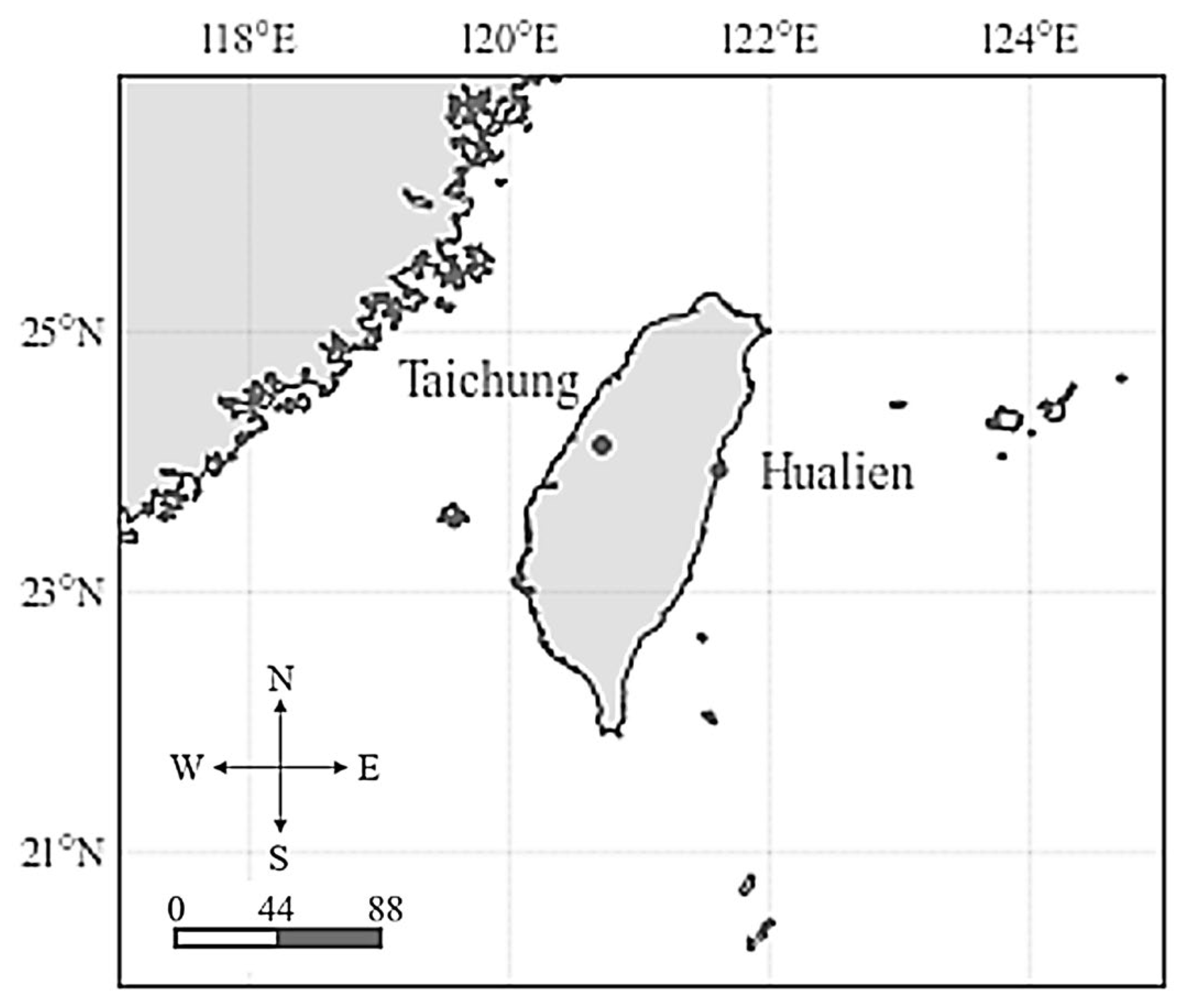
Rainfall records from two ground weather stations in the Taichung and Hualien cities of Taiwan are used (see locations of two stations in Figure 1). These two stations are operated and qualified by Taiwan’s CWA (https://www.cwa.gov.tw/V8/C/ (accessed on 15 March 2024)). A total of 672 monthly rainfall records are available from 1950 to 2005; these records are further divided 3:1:1 for training (January 1950 to December 1983), validation (January 1984 to December 1994) and test (January 1995 to December 2005) purposes.

2.2. GCM Data

GCM output variables from two models, BCC-CSM1.1 and CanESM2, are selected in this work. The backgrounds of these two models are summarized in

Table 1. Details of CANESM2 and BCC-CSM1.1.

Model	CanESM2	BCC-CSM1.1
Horizontal resolution $\left(\mathrm{k}\mathrm{m}\right)\times \left(\mathrm{k}\mathrm{m}\right)$	128 × 64	128 × 64
Output variable number	30	30
Length of historical data	January 1995–December 2005	January 1995–December 2005
Length of scenario data	January 2006–December 2099	January 2006–December 2099
Abbreviation	CAN	BCC

.

In this study, the duration of the historical scenario data is from January 1950 to December 2005, and that of the future scenario data (rcp4.5 and rcp8.5) is from January 2006 to December 2099. The features of AR5 GCMs selected in this study are listed in

Table 2. List of the selected variables used in this work.

Long Name	Output Variable Name
Total Cloud Fraction	clt
Air Pressure at Convective Cloud Base	ccb
Air Pressure at Convective Cloud Top	cct
Cloud Area Fraction	cl
Mass Fraction of Cloud Liquid Water	clw
Condensed Water Path	clwvi
Evaporation	evspsbl
Relative Humidity	hur
Specific Humidity	hus
Surface Upward Latent Heat Flux	hfls
Near-Surface Specific Humidity	huss
Near-Surface Relative Humidity	hurs
Precipitation	pr
Convective Precipitation	pre
Water Vapor Path	prw
Surface Air Pressure	ps
Sea Level Pressure	psl
Surface Downward Longwave Radiation	rlds
Surface Upwelling Longwave Radiation	rlus
Surface Downwelling Clear-Sky Longwave Radiation	rldsc
Surface Upwelling Shortwave Radiation	rsus
Surface Upwelling Clear-Sky Shortwave Radiation	rsuscs
Air Temperature	ta
Near-Surface Air Temperature	tas
Surface Temperature	ts
Eastward Wind	ua
Eastward Near-Surface Wind	uas
Northward Wind	va
Northward Near-Surface Wind	vas
Daily-Mean Near Surface Wind Speed	sfcWind

.

This study employed the method proposed by Li (2006) to separate typhoon-induced precipitation estimates from the total monthly observed precipitation [17]. The Tropical Cyclone Best Track Data from the Joint Tropical Warning Center (JTWC) (https://www.metoc.navy.mil/jtwc/jtwc.html?western-pacific, accessed on 31 January 2024) were collected for the period of 1950–2005. As suggested by Li (2006), the domain covering 117E–125E in longitude and 19N–28N in latitude is defined as the effective typhoon region [17]. The accumulated precipitation observations from the time when a given typhoon center entered this domain through the next six hours was deemed a typhoon; this is defined as an individual typhoon precipitation. The sum of individual typhoon precipitations of all typhoons in a month is thus defined as the monthly typhoon precipitation. Monthly non-typhoon precipitation can therefore be derived by subtracting monthly typhoon precipitation from the monthly precipitation totals.

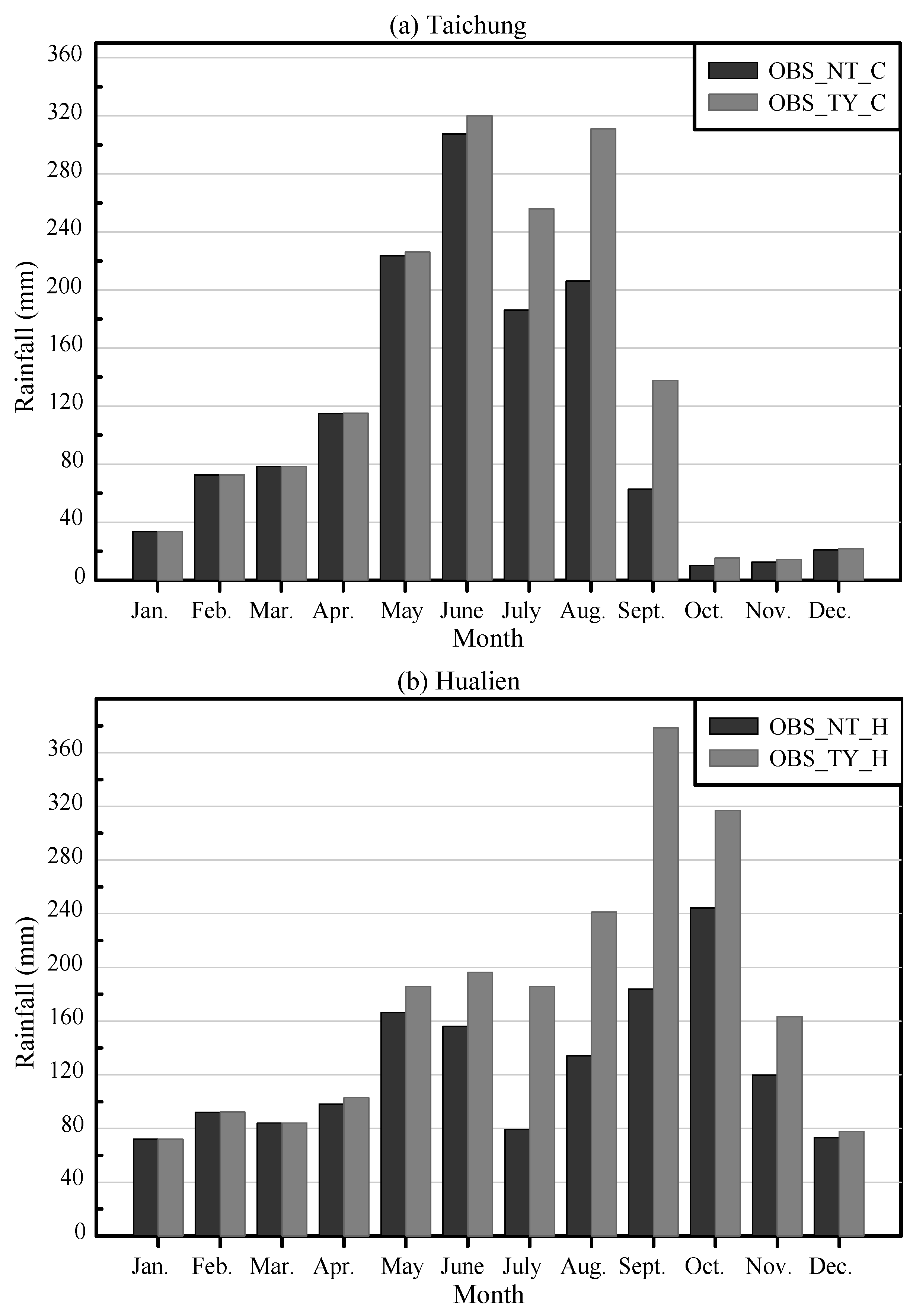
Figure 2 shows the averages of monthly typhoon precipitation (OBS_TY_C, OBS_TY_H) and monthly non-typhoon precipitation (OBS_NTY_C, OBS_NTY_H) calculated from the total monthly observed precipitation in Taichung and Hualien over the period of 1950–2005. As illustrated, in both Taichung and Hualien, the monthly precipitation is largely contributed by typhoons during the summer (from June to September).

3. Methodology

3.1. Overview

The proposed DNN-based downscaling model includes the following key steps:

a.

Application of KPCA to the identification of key input variables to the DNN model;

b.

DNN architecture design, which includes determining the number of hidden layers, the number of neurons in each hidden layer and the neuron activation function;

c.

Optimization of DNN model parameters.

Finally, the model will be assessed using five performance indicators. These are (as shown in Equations (1)–(5)): percentage of underestimation (PU), root mean square error (RMSE), mean absolute error (MeanAE), maximum absolute error (MaxAE) and bias ratio (BR).

$$\mathrm{P}\mathrm{U}=\frac{number of predicted values which are less than observed value}{number of samples}\times 100\mathrm{\%}$$

(1)

$$\mathrm{R}\mathrm{M}\mathrm{S}\mathrm{E}=\sqrt{\frac{\sum {(y_i-\widehat{y_i})}^2}{n}}$$

(2)

$$\mathrm{M}\mathrm{e}\mathrm{a}\mathrm{n}\mathrm{A}\mathrm{E}=\frac{\sum \left|(y_i{-\widehat{y}}_i\right|}{n}$$

(3)

$$\mathrm{M}\mathrm{a}\mathrm{x}\mathrm{A}\mathrm{E}=\mathrm{M}\mathrm{a}\mathrm{x}\left(\left|(y_i{-\widehat{y}}_i\right|\right)$$

(4)

$$\mathrm{B}\mathrm{R}=\frac{\mathrm{M}\mathrm{e}\mathrm{a}\mathrm{n}\mathrm{A}\mathrm{E}}{\mathrm{M}\mathrm{a}\mathrm{x}\mathrm{A}\mathrm{E}}$$

(5)

The details of each step, as well as the model assessment, will be explained in the following sections.

3.2. Identification of Input Variables

3.2.1. Kernel Principal Component Analysis

Kernel Principal Component Analysis (KPCA) is a variant of the widely used Principle Component Analysis (PCA) technique. As suggested by its name, the key difference lies in that a kernel function is introduced into PCA [18]. This study applied KPCA to extract non-linear data features. The basic idea is to first transform non-linear data into a high-dimensional space, so that the data can be converted into linear separable data in the high-dimensional space. Then, data noises are removed on the premise of maintaining data features. Lastly, the original data are replaced by those variables contributing a majority of variations to the original data. These variables are called kernel principal components. The kernel function K used in this study is a radial basis function (RBF) (as shown in Equation (6)). In Equation (6), the value of $\gamma$ determines the dimension of the projective space; ${\mathit{X}}^{\mathit{i}}$ and ${\mathit{X}}^{\mathit{j}}$ are any two sets of original data; ‖∙‖is the norm of the two sets of data and is generally termed the Euclidean distance.

$$K=\mathrm{e}\mathrm{x}\mathrm{p}{(-\gamma ‖{\mathit{X}}^{\mathit{i}}-{\mathit{X}}^{\mathit{j}}‖}^2), 1\le i, j\le n$$

(6)

In the implementation of KPCA, $\gamma$ and the number of kernel principal components (KPCs) are two key meta-parameters that need to be optimized. The value of $\gamma$ affects the projection of data to the corresponding high-dimensional space. To determine its value, this research adopts the automatic parameter selection (APS) method proposed by Li et al. (2010), whereby the gradient descent method was used to efficiently identify the optimal parameter for RBF [19]. In addition, this work determines the optimal number of KPCs based upon the accuracy measures resulting from k-nearest neighbors (KNN) classification [20]. The adopted accuracy measure is defined as follows:

$$\mathrm{A}\mathrm{c}\mathrm{c}\mathrm{u}\mathrm{r}\mathrm{a}\mathrm{c}\mathrm{y}=\frac{\mathrm{A}\mathrm{c}\mathrm{c}\mathrm{u}\mathrm{r}\mathrm{a}\mathrm{t}\mathrm{e}\mathrm{l}\mathrm{y} \mathrm{c}\mathrm{l}\mathrm{a}\mathrm{s}\mathrm{s}\mathrm{i}\mathrm{f}\mathrm{i}\mathrm{e}\mathrm{d} \mathrm{s}\mathrm{a}\mathrm{m}\mathrm{p}\mathrm{l}\mathrm{e}\mathrm{s}}{\mathrm{m}\mathrm{a}\mathrm{p}\mathrm{p}\mathrm{i}\mathrm{n}\mathrm{g} \mathrm{s}\mathrm{a}\mathrm{m}\mathrm{p}\mathrm{l}\mathrm{e}\mathrm{s}}$$

(7)

3.2.2. KPCA for Identifying Key Input Features

In this study, the original data of predictor variables are normalized (as shown in Equation (8)) to ensure that the upper and lower limits of each variable are consistent. After the data are normalized, the model’s iteration speed could be increased, reducing the time for gradient descent. In addition, the features between factors are maintained and scaled to improve the precision of the model. In Equation (8), Z is the normalized value; $\overline{X}$ is the average; $S_x$ is the standard deviation.

$$Z=\frac{X-\overline{X}}{S_x}$$

(8)

As aforementioned, the parameters that need to be optimized in KPCA are $\gamma$ and $n$ (number of kernel principal components). The former is automatically optimized as a kernel function parameter according to the APS. In the BCC model, for Taichung area, the value of $\gamma$ is 0.01894 for non-typhoon precipitation and 0.01931 for the total precipitation. For the Hualien area, the value of $\gamma$ is 0.05273 for non-typhoon precipitation and 0.03945 for total precipitation. In the CAN model, for the Taichung area, the value of $\gamma$ is 0.03339 for non-typhoon precipitation and 0.01872 for total precipitation. For the Hualien area, the value of $\gamma$ is 0.06675 for non-typhoon precipitation and 0.03630 for total precipitation.

After the parameter $\gamma$ is optimized, the original data are transformed using the corresponding kernel functions. The simulated values and actual values of transformed data are then assessed by applying KNN to obtain the accuracy measures (Equation (7)). The number of kernel principal components can then be determined from the value leading to the highest accuracy. A summary of the optimal parameters, resulting from BCC and CAN models and for Taichung and Hualien areas, respectively, is given in

Table 3. The accuracy of using KNN to determine the number of KPC.

Station	GCM Model	Source Of Rainfall Data	Accuracy (%)	KPC
Taichung	BCC	noTy	0.11	23
		Total	0.07	23
	CAN	noTy	0.25	25
		Total	0.10	6
Hualien	BCC	noTy	0.10	12
		Total	0.06	2
	CAN	noTy	0.11	10
		Total	0.36	10

.

3.3. Deep Neural Networks: Architecture Design

Deep learning is a branch of machine learning, and it aims to extract representative features of data through linear or non-linear transformation in multiple artificial neural (AN) processing layers. In addition, deep learning is more time-saving and easier than traditional feature engineering. Therefore, it has been widely applied in various fields. The deep neural networks (DNN) theory aims to implement multiple computing and training operations of different layers and architectures through a mathematical model that simulates the biological nervous system to identify the optimal and most effective deep learning model [21,22,23,24]. Figure 3 shows the concept, comprising the input layer, hidden layer, and output layer. First, n values (X₁, X₂,…, X_n, n ∈ N) are inputted into the input layer of the DNN model; then, multiple computing and training operations are executed through multiple neurons in one or more processing layers in the hidden layer; lastly, the output value (y) is obtained through computing in the output layer.

The basic components of the DNN downscaling model proposed in this study are input variables, neuron link weights, and neuron activation functions. Input values are weighted when passing through the neurons to better highlight the proportion of each weight in training. Therefore, a non-linear activation function should be used to transform the weights into the non-linear state by weight values. Common activation functions include the Sigmoid function (as shown in Equation (9)) and the tanh function (as shown in Equation (10)), where x is the input value of the activation function.

$$f\left(x\right)=\frac{1}{1+e^{-x}}$$

(9)

$$f\left(x\right)=\frac{e^x-e^{-x}}{e^x+e^{-x}}$$

(10)

Assuming M datasets, each of which has n features {($X_1$,$y_1$), ($X_2$,$y_2$), …, ($X_M$,$y_M$), $X_i$ ∈ $R^n$, $y_i$∈$R^1$}, the mapping function ${\Phi }_{DNN}$ ($X_i$) would map input samples $X_i$ to the output features $y_i$. Via the optimization process, the difference between the predicted ($\widehat{y_i}$) and the observed $y_i$ can be minimized, as shown in Equation (11).

$$\mathit{arg}\underset{\mathit{W}}{\mathit{min}}J\left(\mathit{W}\right)=arg \underset{\mathit{W}}{\mathit{min}}\sum _{i=1}^M{‖y_i-\widehat{y_i}‖}_2$$

(11)

Then, the weights ($\mathit{W}$) of transformed data ($X$) are optimized and updated through an optimizer. The optimizer adjusts the weights through the assessment of preliminarily trained values and tagging factors that are obtained through computing in an error function, so that the weight variables of the model can be continuously optimized. Finally, the weights that can minimize the errors of the output values and tagging factors of machine learning can be obtained. Stochastic gradient descent (SGD) is a commonly used parameter optimization method (as shown in Equation (12)), which controls the extent of weight modification by adjusting the learning rate. If the learning rate is higher, the extent of weight modification will be greater; if the learning rate is lower, the extent of weight modification will be smaller. Note that an overly high learning rate may mean that the most optimal solution is ignored, and non-convergence may even occur. An overly low learning rate may, however, lead to a prolonged learning duration.

$${\mathit{W}}_{t+1}={\mathit{W}}_t-lr\nabla J\left(\mathit{W}\right)$$

(12)

where ${\mathit{W}}_t$ is the original weight, ${\mathit{W}}_{t+1}$ is the updated weight, and lr is the learning rate. The value of lr affects the extent of weight modification. $\nabla J\left(\mathit{W}\right)$ is the gradient of the error function $J\left(\mathit{W}\right)$.

AdaGrad and Adam are two adaptive optimizers extended from SGD. AdaGrad is suitable for processing sparse data as it can adjust the value of the learning rate according to the assessed value obtained by modeling each time, and it can then automate weight modification according to the assessed value. At last, in the later stage of modeling, the learning rate will decrease gradually and eventually reach zero. Adam adds deviation correction based on AdaGrad to correct and resolve other learning problems in the later stage of modeling.

Batch size is a unit number of samples to be processed by a DNN for each weight update. It determines the efficiency of DNN model training. To prevent from overfitting, in each training iteration, a proportion of neurons in the hidden layers can be randomly removed, such that only some of the neurons get updated [25]. This process is called dropout.

The parameter optimization procedure in this study was designed with reference to the staged optimization practice in Bai et al. (2016, 2017) to obtain the local optimum [13,26]. In terms of the number of iterations, Bengio (2012) suggested that the minimal number of trainings should be 10,000 [27]. In this study, the number of iterations was set at 50,000. In terms of the number of hidden layers, Liu (2017) suggested the number of hidden layer(s) be one to two [28], while Bai et al. (2016, 2017) indicated that one to three hidden layer(s) should be designed, and parameters should be optimized in a progressive manner [13,26]. As mentioned by Coppola Jr. et al. (2005), if the input layer has n factors, the number of hidden layers and nodes should be 2N + 1 [29]. Therefore, this study started parameter optimization from one layer in a progressive manner, and set the number of nodes to be tested at 10 and 50. The procedure is as follows:

(1)

Choosing an optimizer (AdaGrad or Adam);

(2)

Determining the activation function (sigmoid or tanh);

(3)

Setting the learning rate (ranging from 0.01 to 0.0001);

(4)

Selecting the batch size (ranging from 16 to 64);

(5)

Determining the number of nodes (ranging from 10 to 100).

The following parameters are optimized: the optimizer options are Adagrad and Adam; the activation function options are sigmoid and tanh; the batch size option is 16; and the node number options are 10 and 50.

3.4. Optimization of Model Parameters

The parameter optimization procedure was designed based on the algorithm proposed in Bai et al. (2016, 2017) [13,26]. The optimizer, activation function, and learning rate are optimized. Then, the batch size is optimized after the preceding three are fixed. Lastly, the layer number and node number are optimized. We took the Taichung Weather Station monitoring no-typhoon precipitation in the BCC model as an example. Here, there are four combinations of optimizers and activation functions. The batch size is set at 16, the layer number is set at 1, and the node numbers are set at 10 and 50. The converging trend is determined according to different learning rates and the RMSE is calculated.

Table 4. Assessment results (normalized RMSE) of DNN downscaling models for four input variables.

n_Components = 4 $\mathit{\gamma }$ = 0.0189			Layer	Node	10			50
				Ir	0.01	0.001	0.0001	0.01	0.001	0.0001
C	Adagrad	sigmoid	1	RMSE	1.07403	1.02925	1.16097	1.16673	1.03443	1.16714
		tanh			1.32746	1.19892	0.99706	1.34455	1.02353	1.02408
	Adam	sigmoid	1	RMSE	1.34725	0.99238	1.03060	1.34434	1.16298	1.00758
		tanh			1.33056	1.33417	1.02146	1.32340	1.34432	1.21584
H	Adagrad	sigmoid	1	RMSE	0.85935	0.84993	0.82558	0.85779	0.84836	0.86098
		tanh			0.89153	0.84601	0.86170	0.89997	0.87658	0.86690
	Adam	sigmoid	1	RMSE	0.86541	0.86051	0.82198	0.92920	0.85073	0.81970
		tanh			0.88730	0.89611	0.85805	0.89033	0.89681	0.82764

describes the model optimization assessment. As seen, for the Taichung Weather Station with no-typhoon precipitation, we selected the parameter optimizer Adam, the activation function Sigmoid, a learning rate 0.001, 10 nodes, and one hidden layer.

3.5. Model Assessment

The DNN downscaling model proposed in this study uses two GCMs. Each GCM has two input factors (non-typhoon precipitation and original precipitation) and two weather stations, totaling eight models. The data are divided into 3:1:1 (training: (January 1950 to December 1983), validation (January 1984 to December 1994), and test (January 1995 to December 2005)) by the number of data sets. In the training phase, the aforementioned RMSE is used for assessment and the model is used as the selected model.

Table 5. Assessment results of DNN downscaling models.

GCM Model	Source of the Rainfall Data	Station	Output Variable Number	$\mathit{\gamma }$	Optimizer	Activation Function	Learning Rate	Node	RMSE
BCC	Total	C	23	0.01931	Adagrad	tanh	0.0001	10	1.09106
		H	4	0.03945	Adagrad	tanh	0.001	10	1.12866
	No_typhoon	C	4	0.01894	Adam	sigmoid	0.001	10	0.99238
		H	12	0.05273	Adam	sigmoid	0.0001	50	0.81970
CAN	Total	C	6	0.01872	Adam	sigmoid	0.01	10	0.82479
		H	10	0.03630	Adam	tanh	0.001	10	1.04221
	No_typhoon	C	25	0.03339	Adagrad	sigmoid	0.01	10	0.82064
		H	10	0.06675	Adam	tanh	0.0001	10	0.80403

lists the final optimized parameters for the Taichung (C) and Hualien (H) DNN models, as well the optimal DNN architecture and parameters in view of the original total monthly precipitation (total) and non-typhoon precipitation (no_typhoon) in the BCC and CAN models. From the perspective of dimensionless RMSE, both the Taichung and Hualien DNN models show that non-typhoon precipitation is superior to original total precipitation, the number of nodes is mostly 10, and the number of hidden layers is one. As listed in the Tab., the optimizer is mostly Adam, the activation function is half sigmoid and half tanh, the learning rate is from 0.001 to 0.0001, the number of nodes is mostly 10, and the value of dimensionless RMSE is small.

The associated performance measures are summarized in

Table 6. Performance assessment of the proposed DNN-based downscaling models for BCC and CAN under historical scenarios.

Models	PU (%)	BR
Hualien_BCC_noTy	33	6.31
Hualien_BCC_Total	36	12.33
Hualien_CAN_noTy	31	2.24
Hualien_CAN_Total	37	2.25
Taichung_BCC_noTy	48	5.10
Taichung_BCC_Total	37	7.47
Taichung_CAN_noTy	32	5.69
Taichung_CAN_Total	42	8.58

. As can be seen, in terms of PU, the difference between total and non-typhoon precipitation in Hualien is much smaller than that in Taichung. This confirms the observation summarized in Figure 2 that a larger proportion of precipitation is contributed by typhoons in Hualien. The fact that the BR values resulting from non-typhoon precipitation are generally lower than those from total precipitation also confirms that the proposed method used to separate non-typhoon precipitation from total precipitation is effective.

4. Future Precipitation Assessment

This study further utilizes the proposed DNN-based downscaling model to predict the future precipitation trend and uncertainty for the Taichung and Hualien areas with or without the effect of typhoons. Future scenario data of the BCC and CAN models were input into the DNN model for analysis and assessment. The data duration is from January 2006 to December 2099 (scenarios used are rcp 4.5 and rcp 8.5). Future precipitation analysis is conducted in three parts: (1) three-classification analysis of future scenario precipitation of the weather stations; (2) probability analysis of monthly precipitation; and (3) classification of future scenario data into mid-term (January 2051 to December 2060) and long-term (January 2071 to December 2080), and analysis of monthly precipitation averages and box plots to assess the trend and uncertainty.

4.1. Three-Classification and Range Analysis of Future Scenario Precipitation

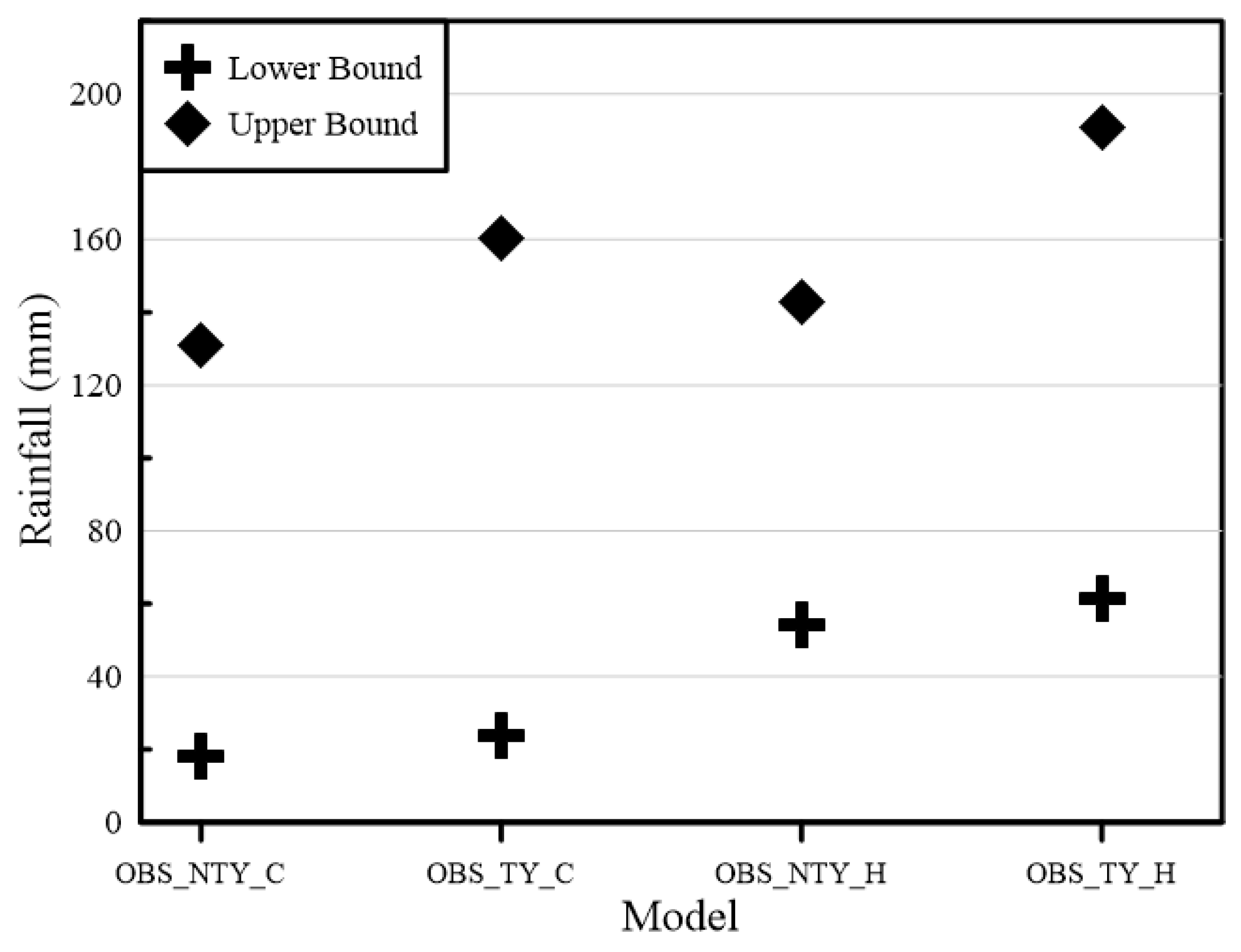
This study applied the climatic forecast three-classification analysis method proposed by the Central Weather Bureau of Taiwan to analyze the future precipitation trend in the BCC and CAN models. In terms of the precipitation three-classification analysis result, 30% and 70% of the precipitation were used as the lower and upper limits of the normal precipitation range. The “normal” category includes the precipitation that falls within the range between the upper and lower limits. The “low” category includes the precipitation that falls below the lower limit. The “heavy” category includes the precipitation that is above the upper limit. Figure 4 shows the upper and lower limits of the historical precipitation three-classification analysis for Taichung and Hualien.

According to the three-classification upper and lower limits of historical precipitation, precipitation classification could be implemented for two scenarios and two models at the Taichung and Hualien weather stations. The model naming rules were GCM_with/without the effect of typhoons_future scenario. For example, BCC_NTY_rcp8.5 denotes that the GCM model is BCC, excluding the effect of typhoons, and the future scenario is rcp 8.5. Similarly, BCC_TY_rcp8.5 denotes that the effect of typhoons is included, and the precipitation properties of the wet season (May to October) precipitation and the dry season (January to April, November, and December) are included, as shown in Figure 5 and Figure 6. Figure 5 shows the three-classification analysis result of future wet and dry season precipitation for the Taichung area. As shown in Figure 5, the wet and dry season precipitation in two scenarios (rcp 4.5 and rcp 8.5) is affected by typhoons. Each DNN model presents roughly the same trend: the wet season precipitation is less significantly affected by typhoons. The BCC model shows that in any scenario, the wet season precipitation is too much, whereas the dry season precipitation is too low. The CAN model shows a small wet-to-dry season precipitation variation. Figure 6 shows the three-classification analysis result of future wet and dry season precipitation for Hualien. As seen, each DNN downscaling model has nearly the same trend: the wet season precipitation is less significantly affected by typhoons, whereas the dry season precipitation in the rcp 8.5 scenario is more significantly affected by typhoons than that in the rcp4.5 scenario. Overall, the summer precipitation is mostly within the normal range for both Taichung and Hualien weather stations, and the winter precipitation is mostly too much for Taichung, and is half normal and half too much for Hualien.

Figure 7 shows the precipitation range prediction results, including the results with and without the effects of typhoons. The mid-term precipitation is mostly within 100 mm to 200 mm for both Taichung and Hualien. The long-term precipitation is mostly within 100 mm to 200 mm for Taichung and generally within 0 mm to 100 mm and 100 mm to 200 mm for Hualien.

4.2. Future Scenario Precipitation Assessment

Figure 8 shows the future monthly precipitation prediction for Taichung and Hualien. The model naming rules are: mid-term/long-term or observation (obs)_with or without typhoons_station. M/L represents mid-term/long-term, Ty/nTy denotes with/without typhoons, and C/H denotes Taichung Weather Station/Hualien Weather Station. According to the mid-term precipitation prediction for Taichung shown in the Figure 8, the wet season precipitation in the two models is below the historical average, whereas the dry season precipitation in the two models is above the historical average, and the dry season variation is great. According to the long-term precipitation prediction for Taichung, the wet season precipitation variation is small, whereas the dry season precipitation variation is great. The dry season precipitation is less significantly affected by typhoons and the long-term wet season precipitation is more significantly affected by typhoons than the mid-term wet season precipitation. According to the mid-term precipitation prediction for Hualien, the dry season precipitation variation is greater than the wet season precipitation variation. The model without the effect of typhoons shows a precipitation trend that is more approximate to the historical precipitation trend. According to the mid- and long-term precipitation predictions for Hualien, the dry season precipitation variation is greater than the wet season precipitation variation, and the long-term wet season precipitation is more significantly affected by typhoons. Overall, the mid-term dry season precipitation variation is greater than the mid-term wet season precipitation variation for both Taichung and Hualien, and the long-term precipitation variation is greater than the mid-term precipitation variation.

Figure 9 shows the probability of the long-term monthly precipitation prediction exceeding the historical average for the two weather stations. As shown in the figure for the Taichung area, the mid-term/long-term precipitation is below the historical average in May, June, and August, and above the historical average in July. This indicates that the probability of falling below the historical average of future wet season precipitation for Taichung is high. The dry season monthly precipitation is above the historical average, and typhoon precipitation is higher than no-typhoon precipitation, indicating that for the Taichung area, the future precipitation has a higher probability of being affected by typhoons due to climate change. The precipitation trend for Hualien is the same as that for the Taichung area, except for the fact that the dry season monthly precipitation for Hualien is less significantly affected by typhoons. Overall, for both Taichung and Hualien areas, the mid-term/long-term dry season precipitation has a much higher probability of exceeding the historical average than the wet season precipitation. The dry season precipitation for Taichung is more significantly affected by typhoons than that for Hualien.

5. Conclusions

This study applied KPCA to extract non-linear features of high-dimensional data as inputs of the DNN model, so as to reduce the model complexity and data noise. A DNN-based downscaling model was designed for monthly precipitation. This study selected the BCC-CSM1.1 model and CanESM2 model from the IPCC AR5 models, and conducted a case study of Taichung and Hualien. The following conclusions were drawn:

• For both Taichung and Hualien DNN downscaling models, the number of hidden layers is 1, the learning rate ranges from 0.001 to 0.0001, and the number of nodes is mostly 10;
• The DNN downscaling models were BCC and CAN models. Dimensionless RMSE shows opposite trends for Taichung and Hualien. Specifically, for the Hualien area, the performance of the BCC model is superior to that of the CAN model, and for the Taichung area, the performance of the CAN model is superior to that of the BCC model;
• According to the three-classification analysis of future scenario precipitation predictions, the summer precipitation for both Taichung and Hualien weather stations is mostly within the normal range, whereas the winter precipitation for Taichung is mostly too much, and the winter precipitation for Hualien is half normal and half too much;
• According to the analysis of future precipitation ranges, the mid-term precipitation for both Taichung and Hualien is mostly within 100 mm to 200 mm, while the long-term precipitation is mostly within 100 mm to 200 mm for Taichung and is generally within 0 mm to 100 mm and 100 mm to 200 mm for Hualien;
• According to the analysis of future monthly precipitation, the wet season precipitation is below the historical average and the dry season precipitation is above the historical average. For both Taichung and Hualien areas, the dry season precipitation variation is greater than the wet season precipitation variation and the long-term precipitation variation is greater than the mid-term precipitation variation. For the Taichung area, the long-term dry season precipitation is less significantly affected by typhoons and the long-term wet season precipitation is more significantly affected by typhoons. For Hualien mid-term precipitation, the model without the effect of typhoons shows a mid-term precipitation trend closer to the historical precipitation trend and the long-term wet season precipitation is more significantly affected by typhoons;
• According to the analysis of the probability of the future monthly precipitation exceeding the historical monthly average precipitation, for both the Taichung and Hualien areas, the mid-term/long-term dry season precipitation has a much higher probability of exceeding the historical average than the wet season precipitation, and the dry season precipitation for Taichung is more significantly affected by typhoons than that in Hualien.

References

- Field, C.B.; Barros, V.R. (Eds.) Climate Change 2014—Impacts, Adaptation and Vulnerability: Regional Aspects; Cambridge University Press: Cambridge, UK, 2014. [Google Scholar]
- Kitoh, A.; Endo, H.; Krishna Kumar, K.; Cavalcanti, I.F.; Goswami, P.; Zhou, T. Monsoons in a changing world: A regional perspective in a global context. J. Geophys. Res. Atmos. 2013, 118, 3053–3065. [Google Scholar] [CrossRef]
- Chou, C.; Liu, S.C. Observations of Global Climate Changes. Atmos. Sci. 2012, 40, 185–213. Available online: https://www.airitilibrary.com/Article/Detail?DocID=02540002-201209-201303010037-201303010037-185-213 (accessed on 11 March 2024).
- Huang, W.C.; Chiang, Y.; Wu, R.Y.; Lee, J.L.; Lin, S.H. The impact of climate change on rainfall frequency in Taiwan. Terr. Atmos. Ocean. Sci. 2012, 23, 553–564. [Google Scholar] [CrossRef]
- Giorgi, F.; Mearns, L.O. Approaches to the simulation of regional climate change: A review. Rev. Geophys. 1991, 29, 191–216. [Google Scholar] [CrossRef]
- Wilby, R.L.; Dawson, C.W.; Barrow, E.M. SDSM—A decision support tool for the assessment of regional climate change impacts. Environ. Model. Softw. 2002, 17, 145–157. [Google Scholar] [CrossRef]
- Lin, S.S.; Hu, Y.L.; Zhu, K.Y. Downscaling model for rainfall based on the influence of typhoon under climate change. J. Water Clim. Change 2022, 13, 2443–2458. [Google Scholar] [CrossRef]
- Li, C.Y.; Lin, S.S.; Chuang, C.M.; Hu, Y.L. Assessing future rainfall uncertainties of climate change in Taiwan with a bootstrapped neural network-based downscaling model. Water Environ. J. 2020, 34, 77–92. [Google Scholar] [CrossRef]
- Maraun, D. Bias correction, quantile mapping, and downscaling: Revisiting the inflation issue. J. Clim. 2013, 26, 2137–2143. [Google Scholar] [CrossRef]
- Li, C.Y.; Lin, S.S.; Lin, Y.F.; Kan, P.S. A bootstrap regional model for assessing the long-term impacts of climate change on river discharge. Int. J. Hydrol. Sci. Technol. 2019, 9, 84–108. [Google Scholar] [CrossRef]
- Aswin, S.; Geetha, P.; Vinayakumar, R. Deep learning models for the prediction of rainfall. In Proceedings of the 2018 International Conference on Communication and Signal Processing (ICCSP), Chennai, India, 3–5 April 2018; IEEE: Piscataway, NJ, USA; pp. 0657–0661. [Google Scholar] [CrossRef]
- Basha, C.Z.; Bhavana, N.; Bhavya, P.; Sowmya, V. Rainfall prediction using machine learning & deep learning techniques. In Proceedings of the 2020 International Conference on Electronics and Sustainable Communication Systems (ICESC), Coimbatore, India, 2–4 July 2020; IEEE: Piscataway, NJ, USA; pp. 92–97. [Google Scholar] [CrossRef]
- Bai, Y.; Chen, Z.; Xie, J.; Li, C. Daily reservoir inflow forecasting using multiscale deep feature learning with hybrid models. J. Hydrol. 2016, 532, 193–206. [Google Scholar] [CrossRef]
- Hinton, G.E.; Salakhutdinov, R.R. Reducing the dimensionality of data with neural networks. Science 2006, 313, 504–507. [Google Scholar] [CrossRef]
- Debruyne, M.; Hubert, M.; Van Horebeek, J. Detecting influential observations in Kernel PCA. Comput. Stat. Data Anal. 2010, 54, 3007–3019. [Google Scholar] [CrossRef]
- Jolliffe, I.T.; Cadima, J. Principal component analysis: A review and recent developments. Philos. Trans. R. Soc. A Math. Phys. Eng. Sci. 2016, 374, 20150202. [Google Scholar] [CrossRef] [PubMed]
- Li, Y.C. The Analysis of Climatological Characteristics of Non-Typhoon Rainfall in Taiwan. Master’s Thesis, National Taiwan University, Taipei, Taiwan, 2006. [Google Scholar] [CrossRef]
- Schölkopf, B.; Smola, A.; Müller, K.R. Nonlinear component analysis as a kernel eigenvalue problem. Neural Comput. 1998, 10, 1299–1319. [Google Scholar] [CrossRef]
- Li, C.H.; Lin, C.T.; Kuo, B.C.; Chu, H.S. An automatic method for selecting the parameter of the RBF kernel function to support vector machines. In Proceedings of the 2010 IEEE International Geoscience and Remote Sensing Symposium, Honolulu, HI, USA, 25–30 July 2010; IEEE: Piscataway, NJ, USA; pp. 836–839. [Google Scholar] [CrossRef]
- Fix, E.; Hodges, J.L. Discriminatory analysis. Nonparametric discrimination: Consistency properties. Int. Stat. Rev. Rev. Int. Stat. 1989, 57, 238–247. [Google Scholar] [CrossRef]
- Rumelhart, D.E.; Hinton, G.E.; Williams, R.J. Learning representations by back-propagating errors. Nature 1986, 323, 533–536. [Google Scholar] [CrossRef]
- Schmidhuber, J. Deep learning. Scholarpedia 2015, 10, 32832. [Google Scholar] [CrossRef]
- LeCun, Y.; Bengio, Y.; Hinton, G. Deep learning. Nature 2015, 521, 436–444. [Google Scholar] [CrossRef]
- Goodfellow, I.; Bengio, Y.; Courville, A. Deep Learning; MIT Press: Cambridge, MA, USA, 2016. [Google Scholar]
- Hawkins, D.M. The problem of overfitting. J. Chem. Inf. Comput. Sci. 2004, 44, 1–12. [Google Scholar] [CrossRef]
- Bai, Y.; Sun, Z.; Zeng, B.; Deng, J.; Li, C. A multi-pattern deep fusion model for short-term bus passenger flow forecasting. Appl. Soft Comput. 2017, 58, 669–680. [Google Scholar] [CrossRef]
- Bengio, Y. Practical recommendations for gradient-based training of deep architectures. In Neural Networks: Tricks of the Trade: Second Edition; Springer: Berlin/Heidelberg, Germany, 2012; pp. 437–478. [Google Scholar] [CrossRef]
- Liu, F.; Xu, F.; Yang, S. A flood forecasting model based on deep learning algorithm via integrating stacked autoencoders with BP neural network. In Proceedings of the 2017 IEEE third International Conference on Multimedia Big Data (BigMM), Laguna Hills, CA, USA, 19–21 April 2017; IEEE: Piscataway, NJ, USA; pp. 58–61. [Google Scholar] [CrossRef]
- Coppola, E.A., Jr.; Rana, A.J.; Poulton, M.M.; Szidarovszky, F.; Uhl, V.W. A neural network model for predicting aquifer water level elevations. Groundwater 2005, 43, 231–241. [Google Scholar] [CrossRef]
Figure 1.
Geographical locations of the weather stations.
Figure 2.
Averages of monthly typhoon (OBS_TY_C) and non-typhoon (OBS_NT_C) precipitation at Taichung and Hualien weather stations.
Figure 3.
The architecture of the deep neural network (ellipsis of input/output layer or neuron, three black dots in a row; neuron, White dot).
Figure 4.
Upper and lower limits of the normal range of historical precipitation of Taichung and Hualien weather stations.
Figure 5.
Three-step classification of the long-term wet and dry season precipitation in the Taichung model.
Figure 6.
Three-step classification of the long-term wet and dry season precipitation in the Hualien model.
Figure 7.
Probabilities of the long-term wet and dry season precipitation ranges in the Taichung and Hualien models.
Figure 8.
Future scenario (mid-term and long-term) precipitation predictions with and without typhoons for Taichung and Hualien weather stations.
Figure 9.
Probability of the future scenario (mid-term and long-term) monthly precipitation exceeding the historical average with or without typhoon precipitation for Taichung and Hualien.