
Modulation of the Madden–Julian Oscillation Center Stagnation on Typhoon Genesis over the Western North Pacific

1
College of Ocean and Meteorology, Guangdong Ocean University, Zhanjiang 524088, China
2
Shenzhen Institute of Guangdong Ocean University, Shenzhen 518120, China
*
Author to whom correspondence should be addressed.
†
Chun-qiao Lin (2000-), female, M.S. student, research interests in sea-air interactions.
Atmosphere 2024, 15(3), 373; https://doi.org/10.3390/atmos15030373
Submission received: 4 February 2024
/
Revised: 14 March 2024
/
Accepted: 15 March 2024
/
Published: 18 March 2024
(This article belongs to the Section Meteorology)
Abstract
:Madden–Julian Oscillation (MJO) modulates the generation of typhoons (TYs) in the western North Pacific (WNP). Using IBTrACS v04 tropical cyclone best path data, ERA5 reanalysis data, and the MJO index from the Climate Prediction Center (CPC), this paper defines an index to describe the persistent anomalies of the MJO and to examine the statistical characteristics of TYs over 44 years (1978–2021), focusing on the analysis of major differences in environmental conditions after the removal of the ENSO signal over the WNP. The results indicate that the persistent anomalous state of the MJO influences the change in large-scale environmental factors, which, in turn, affects the generation of TYs, as follows: (1) For the I high-value years, the center of the MJO stagnates in the Indian Ocean–South China Sea (SCS), the monsoon trough retreats westward, the warm pool becomes warmer, and the Walker circulation is enhanced. There is stronger upper-level divergence and low-level convergence, larger low-level relative vorticity, higher mid-level relative humidity, and smaller vertical wind shear in the SCS and the seas near the Philippines. Consequently, these conditions foster a conducive environment for TY genesis in the SCS and the seas near the Philippines. (2) For the I low-value years, the center of the MJO stagnates in the WNP–North America region, the monsoon trough extends eastward, the warm pool becomes colder, and the Walker circulation is weakened. Consequently, these conditions are more likely to facilitate TY genesis in the central–eastern WNP. The results show that persistent anomalies in MJO active centers can effectively improve the predictive ability of TY frequency.
1. Introduction
Tropical Cyclones (TCs) are among the most destructive natural disasters [1]. The western North Pacific (WNP) is the world’s most active region of TCs. Approximately 26 named TCs per year over the WNP basin often cause extreme events, such as violent winds and heavy rains, resulting in unquantifiable property damage and human casualties in coastal countries [2,3,4]. Given the context of global warming, studying the long-term variations in TC activity in the WNP is significant [5,6].
Previous studies have shown that the El Niño Southern Oscillation (ENSO) is the strongest interannual signal from tropical air–sea systems, modulating TC activity by changing large-scale circulation [7,8]. Ramage et al. suggest that the eastward movement of tropical cyclone position in El Niño years and the opposite in La Niña years may be related to the equatorial east–central Pacific Sea Surface Temperature (SST) [9]. Chan et al. also found that tropical cyclone activity was more active and stronger in El Niño years [10].
TC activity is characterized by multiple time scales. The Madden–Julian Oscillation (MJO), with a period of 30–90 days, significantly influences TC activity [11]. Gray et al. found, for the first time, that global TC activity exhibits a prominent cluster and periodicity, showing that TCs typically occur in concentrated periods of 1–2 weeks, followed by rare occurrences in the subsequent 2–3 weeks [12]. Subsequently, numerous studies have shown that TCs in different global seas are prone to be generated during the convectively active phase of the MJO [13,14]. Liebmann et al. indicated that when the convective center of the MJO is in the fifth and sixth phases (the western equatorial Pacific), the frequency of TCs in the WNP is greater [15]. Li et al. found that when the convection center of the MJO was in the second and third phases, the dynamic factors in the WNP showed a trend of inhibiting convection and TC development, whereas when the center is in the fifth and sixth phases, the factors show a tendency to promote convection and favor TC development [16]. Zhou et al. further analyzed the large-scale circulation field at different phases of the MJO and found that the large-scale circulation field is significantly different at different phases of the MJO, thus affecting the generation and development of TCs [17].
Previous studies have primarily concentrated on the effects of the MJO phases on TCs, with less emphasis on the impact of MJO center positions on TC genesis. Therefore, this paper focuses on the modulation of TYs by MJO activity centers in specific regions, following the removal of ENSO signals, to provide a reference for TY prediction on a seasonal scale.
2. Data and Methods
2.1. Data
We extracted the TC information from the International Climate Management Best Track Archive (IBTrACS v04) [18]. The data had a temporal resolution of 6 h and contained the central position and the central maximum wind speed. ERA5 provided monthly mean atmospheric reanalysis data for the period 1940–2021, with a horizontal resolution of 0.25° × 0.25°, including 850 hPa relative vorticity and 600 hPa relative humidity [19]. Global monthly mean SST data for 1870–2021 were provided by the Hadley Centre, with a spatial resolution of 1.0° × 1.0° [20]. The Climate Prediction Center (CPC) provided the MJO index for 1978–2021 [21]. The MJO index from the CPC had a time resolution of five days. Based on the extended empirical orthogonal function (EEOF) of the velocity potential at 200 hPa, 10 MJO indices were defined by projecting the data onto the 10 spatial fields of the first mode of the EEOF, corresponding to the locations of the 10 MJO centers of convective activity (80° E, 100° E, 120° E, 140° E, 160° E, 120° W, 40° W, 10° W, 20° W, and 70° W) [22]. Thus, the MJO index from the CPC represents the variation of MJO convective activity centers in different regions, including the tropical Indian and western Pacific oceans. The Real-time Multivariate MJO (RMM) index focuses more on the process of MJO propagation and is only an approximate indication of the location of its center of activity [23]. Compared to the RMM index, the MJO index from the CPC is more reliable in characterizing the active status of the MJO at specific locations [24].
2.2. Method
According to the criteria defined by Joint Typhoon Warning Center (JTWC), the time and location of the central wind speed of TCs ≥ 34 m/s (64 kn) are defined in this paper as the time and location of typhoon (TY) genesis. Wang et al. define the season of TY occurrence in the WNP as May to November; therefore, this paper focuses on the MJO activity from May to November [25].
To preserve the periodic oscillation characteristics of the large-scale environmental fields at intra-seasonal time scales, while simultaneously isolating most of the ENSO signals, a 30–60 d Lanczos band-pass filter was applied to all large-scale environmental factors. The Lanczos time filtering method is a widely used band-pass filter in meteorology [26]. It is a time series x(t) at time t, which is transformed into a time series y(t) by linear processing, and the expression is as follows:
To filter out the frequency band [f1, f2], the weighting factor w(t) needs to be calculated as follows:
In this study, we defined an index that expresses the activity of the MJO from May to November in the WNP. As shown in Equation (3), the I index that describes the persistent anomalies of the center of the MJO is calculated from the IMJO
index from the CPC, and the expression is as follows:
We selected the CPC-MJO daily data for May to November of a specific year to calculate the I index. Then, we averaged the I index from May to November to obtain the average I value for that specific year. IMJO120°E and IMJO160°E represent the active degree of the MJO in the South China Sea (SCS) and the WNP. The negative value of the MJO index from the CPC indicates the MJO convective active phase, and the positive value indicates the MJO convective inhibited phase. Therefore, if I is positive, the MJO is more active in the SCS than the MJO in the WNP, and if I is negative, the MJO is more active in the WNP than the MJO in the SCS. The larger the absolute value of I, the more significant the MJO activity. In addition, the statistical tests used were Student’s t-tests.
3. Results
3.1. MJO Activity Characteristics
The calculated index was used to make a time evolution chart from 1978 to 2021 (Figure 1). The years with greater than 0.5 standard deviations were selected as the I high-value years, i.e., the years where the MJO was mainly active in the SCS, and the years with less than −0.5 standard deviations were selected as the I low-value years, i.e., the years where the MJO was mainly active over the WNP. The years with high and low values are shown in Table 1.
From May to November in the I high-value years, the MJO stagnated in the Indian Ocean–SCS region (80° E–120° E) (Figure 2a). The activity center of the MJO stagnated in the Indian Ocean–SCS region from May. Subsequently, the intensity of the MJO increased, and the range of the center expanded. A brief weakening in the intensity of the MJO center occurred at the end of July. The MJO intensity (−1) in August was the strongest of the year and began to move eastward, and the MJO moved eastward to the eastern Pacific Ocean (120° W) in November. The MJO stagnated in WNP–North America (160° E–40° W) from June to November in the I low-value years (Figure 2b), and the intensity (−0.5) of the center throughout the year was weak. The center of MJO activity stagnated in the Pacific region from June. From July to August, the range of the MJO center narrowed, and the intensity remained the same. The MJO center started moving eastward in September, and the MJO center returned to the Pacific region in November. From the composite plot of the differences between the MJO index from the CPC in the I high- and low-value years (Figure 2c), the index defined in this paper reflects the persistent stagnation of the MJO from May to November, and it corresponds well with the two key zone ranges (120° E and 160° E) for index selection. The center of the negative difference was located in the Indian Ocean–SCS region (80° E–120° E), and the center of the positive difference was located in WNP–North America (160° E–40°W). The intensity of the MJO varied inversely in two key areas: when the center of MJO activity was stagnant in the SCS, i.e., the MJO was continuously active in the SCS, the intensity of the MJO over the WNP was continuously weak, whereas when the center of MJO activity was stagnant over the WNP, i.e., the MJO was continuously active in the WNP, the intensity of the MJO in the SCS was continuously weak.
3.2. Statistical Characteristics of TYs in the WNP
The average frequency of TYs in the I low-value years (15.1 per year) was greater than that of TYs in the I high-value years (13 per year). The annual tropical cyclone frequency was generally above the average in the I low-value years, whereas it was below the average in almost half of the I high-value years (Figure 3).The location of TY genesis in Figure 4 shows that a significant number of TYs were generated in the range of 140° E–180° E in the I low-value years, whereas TYs in the I high-value years were generated in the area west of 140° E. According to statistics, there were 137 TYs in the I high-value years, of which 106 TYs (77% of the total) were produced between 100° E and 140° E, and 31 TYs (23% of the total) were produced between 140° E and 180° E. There were 181 TYs in the I low-value years, of which 101 TYs were produced between 100° E and 140° E, accounting for 56% of the total, and 80 TYs were produced between 140° E and 180° E, accounting for 44% of the total (Table 2). Compared to the I high-value years, the proportion of TYs generated east of 140° E increased in the I low-value years.
It is clear that the center of the MJO in the I high-value years stagnated in the Indian Ocean–SCS, the annual mean TY frequency in the WNP was low, and the genesis location was mainly in the region of the SCS and the seas near the Philippine Islands. The center of the MJO in the I low-value years stagnated in WNP–North America, the annual mean TY frequency in the WNP was high, and the genesis location was mainly in the region east of the Philippines in the WNP. This shows that the MJO has an important modulation effect on TYs in the WNP, and the frequency and position of TYs change with movement of the MJO active center. The MJO influences the development of TCs by changing the environmental conditions [27,28]. Therefore, in this paper, we conducted a synthetic analysis of each element in the I high- and low-value years to explore how the MJO influences TYs, considering the environmental conditions.
4. Differences in Background Fields between I High- and Low-Value Years
4.1. The Differences in the Warm Pool
Chen et al. found that when the western Pacific warm pool (125° E–165° E, 0°–16° N) is in a warm state, it favors for development of the MJO, providing a favorable dynamical environment for TC formation. Consequently, more TCs are generated on the western side of the WNP. Conversely, when the WNP warm pool is in a cold state, the MJO activity is weakened and TC activity is suppressed. Consequently, the number of TCs on the southeast side of the WNP is higher [29]. Areas with SST above 28.5 °C are favorable for the generation of TCs. Figure 5a,b shows the mean SST distribution for May–November in the I high- and low-value years, respectively. As seen in Figure 5, the 28.5 °C isotherm was south of 20° N in both the I high- and low-value years. The 29.5 °C isotherm for the I high-value years was located south of 18° N and west of 150° E (Figure 5a), whereas the 29.5 °C isotherm for the I low-value years was located near the equator (10° N–10° S) and east of 140° E (Figure 5b). Compared to the I low-value years, the 29.5 °C isotherm covered a larger area and the location was more westward in the I high-value years. The average warm pool (125° E–145° E, 0°–15° N) temperature was generally higher in the I high-value years (approximately 29.5 °C) than in the I low-value years (approximately 28.5 °C). This disparity could be one of the reasons for the more westward genesis position of TYs in the I high-value years.
4.2. The Differences in Monsoon Trough
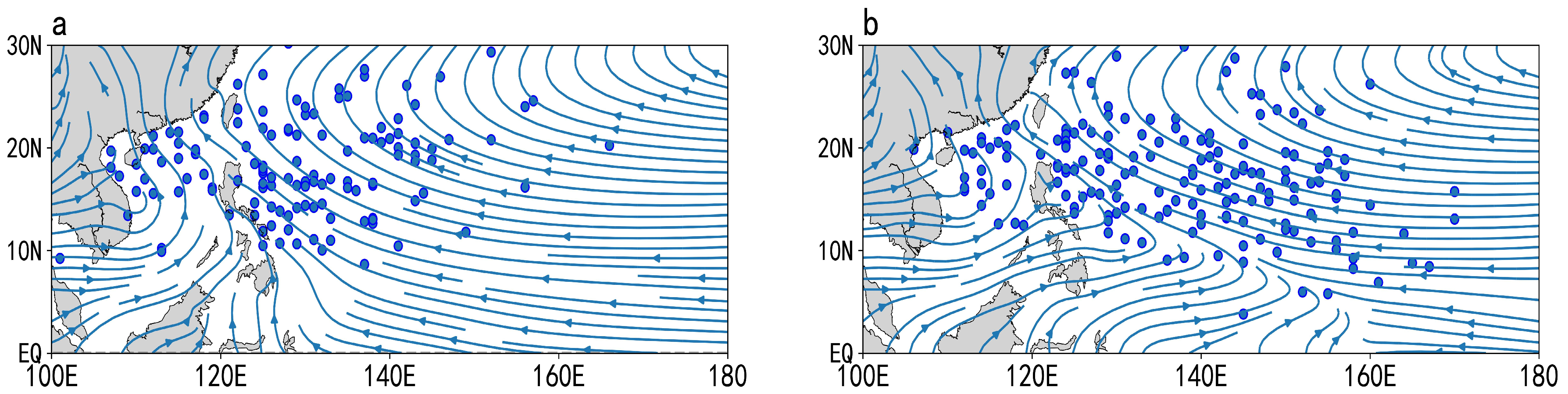
The MJO and the monsoon trough are closely related. The monsoon trough is closely related to the generation, activity, and path of TCs. When the monsoon trough extends eastward (retreats westward), the formation of TCs in the southeast of the WNP increases (decreases) [30,31]. It can be assumed that the MJO has an indirect effect on TCs by influencing the activity of the monsoon trough. Figure 6 shows the 850 hPa mean streamline distribution for these two periods. During high-value years, the monsoon trough receded westward near Luzon, with less pronounced curvature. The southwesterly flow in the south of 15° N was stronger, whereas the southeasterly flow in the north of 15° N was weaker, resulting in weaker shear in the horizontal wind field, with the shear line extending to only 120° E (Figure 6a). In the I low-value years, the monsoon trough exhibited a significant northwest–southeast trend, and the southwest monsoon flow gradually changed to southeast when it reached the middle of the tropical WNP, thus forming a horizontal shear between the southwest monsoon flow and the southeast flow in the WNP. Finally, the trough line of the monsoon trough extended to 150° E in the southeast direction (Figure 6b). TY genesis locations (indicated by the blue dots in Figure 6) predominantly occurred in the monsoon convergence zone at the monsoon trough’s eastern end, with genesis locations shifting alongside the monsoon trough’s movements. In the I high-value years, retreat of the monsoon trough caused the generation position of TYs to shift westward, resulting in an increase in TY generation in the SCS and a decrease in TY generation in the WNP. In the I low-value years, the monsoon trough extended latitudinally up to 150° E, and more TYs occurred in the eastern part of the WNP.
4.3. The Differences in the Walker Circulation
Figure 7 shows the differences in the mean vertical velocity between 5° N and 15° N in the I high- and low-value years. The figure shows that the SCS and the seas near the Philippine Islands were dominated by anomalous updrafts, whereas the WNP was dominated by anomalous downdrafts during the I high-value years. This resulted in an anomalous situation for the Walker circulation and the Walker circulation was enhanced. On the contrary, in the I low-value years, the anomalous downdraft was in the SCS and the sea near the Philippine Islands, and the updraft was in the WNP, creating an anti-Walker circulation situation, which weakened the Walker circulation. Compared with the I low-value years, the rising branch of the Walker circulation in the SCS and the seas near the Philippine Islands was enhanced in the I high-value years, which was favorable for the formation of TYs in the SCS and the seas near the Philippine Islands. Therefore, the location of TY formation in the I high-value years was mainly concentrated west of 140° E and less east of 140° E (Figure 5).
5. Differences in Large-Scale Environmental Elements between I High- and Low-Value Years
5.1. The Differences in Dynamic Factors
High- and low-altitude convergence and divergence are essential dynamical features of TCs [32]. Figure 8 shows the differences between the wind and divergence fields at 850 hPa (Figure 8a) and 200 hPa (Figure 8b) for the I high- and low-value years. In I high-value years, there was upper-level divergence in the SCS, leading to convergence in the lower-level troposphere and enhanced upward motion, which is conducive to the generation of TYs (Figure 8a). In I high-value years, there was lower tropospheric convergence and upper tropospheric divergence in the SCS, which is favorable for the strengthening of convective activity in this region. Consequently, this was favorable for the generation of TYs in the SCS (Figure 8b). In terms of the wind field, at 850 hPa, the Walker circulation caused a low-level easterly wind anomaly in the equatorial western Pacific, which led to an anticyclonic circulation anomaly in the low-level WNP. At 200 hPa, upper-level southerly wind anomalies existed in the SCS. Cyclonic circulation anomalies existed in the upper levels of the WNP. Thus, in I high-value years, anomalous lower-level anticyclonic circulation and anomalous upper-level cyclonic circulation in the WNP region suppressed TY genesis; therefore, TYs are prone to be generated in the SCS.
The lower-level cyclonic relative vorticity in the troposphere over the WNP can provide large-scale convergent upward motion for the development of TCs, which plays a crucial role in the development of TCs [33,34]. Figure 9 shows the mean 850 hPa relative vorticity differences over the northwest Pacific Ocean. It can be seen that the positive vorticity anomaly in the SCS was small in extent, whereas the relative vorticity in the western Pacific was negative. This indicates that the positive relative vorticity in the I high-value years was mainly distributed in the SCS and the seas near the Philippine Islands at low latitudes (south of 10° N). The distribution of positive relative vorticity in the lower-level troposphere was more westward in the I high-value years than in the I low-value years. This is one of the reasons why TYs in I high-value years tend to be generated west of the WNP.
Excessive vertical wind shear inhibits the development of convective activity, which is detrimental to TC genesis. Thus, TCs tends to be generated in areas with low vertical wind shear [35]. Figure 10 shows the differences in vertical wind shear between the I high- and low-value years. In the west–central WNP, the vertical wind shear was significantly smaller in the I high-value years than in the I low-value years, especially in the 0°–15° N, 120° E–150° E area. During the I high-value years, the vertical wind shear in the SCS was smaller, and the larger vertical wind shear in the WNP led to an increased frequency of TC genesis in the SCS and a decreased frequency in the WNP.
5.2. The Differences in Thermodynamic Factors
Water vapor is an important environmental factor for TC genesis. Low relative humidity in the middle troposphere of a region hampers the release of latent heat from condensation and the strengthening of upward motion, thus inhibiting TC development [36]. Figure 11 shows the differences in relative humidity between the I high- and low-value years. As depicted in Figure 11, we can see that there was a positive difference area in the western side of the WNP and the SCS. This indicates that in the seas near the Philippine Islands and the SCS, the relative humidity in the mid-level troposphere was significantly higher during the I high-value years than during the I low-value years. Therefore, TYs in the I high-value years tend to be generated in the western WNP.
6. Conclusions and Discussion
6.1. Conclusions
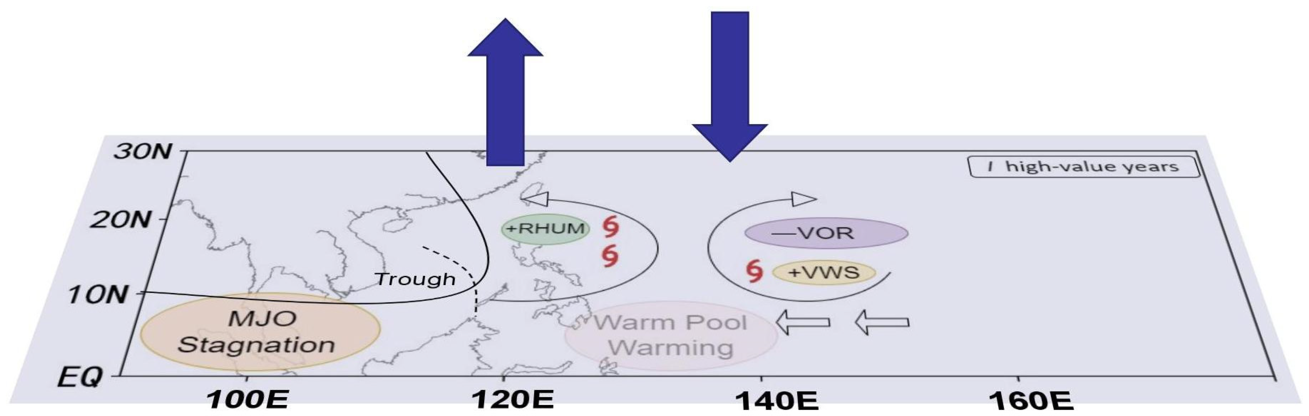
In this paper, we first used the MJO index from the CPC to classify I high- and low-value years using statistical methods. The, we analyzed the MJO activity characteristics of I high- and low-value years, as well as the statistical characteristics of TYs. The results show that in the I high-value years, the MJO stagnated in the Indian Ocean–SCS region, the annual mean TY frequency of the WNP was low, and the TYs tended to occur over the area from the SCS to the seas near the Philippine Islands. In the I low-value years, the MJO stagnated in WNP–North America region, the annual mean TY frequency of the WNP was high, and the TYs tended to occur in the area east of the Philippines on the WNP (Figure 12).
This study also used ERA5 reanalysis data to compare the differences in the background and large-scale environmental fields over the WNP from May to November in I high- and low-value years. We discussed the possible influence of the location of TY genesis. We note that the persistent anomalous state of the MJO will influence the change in large-scale environmental factors, which, in turn, will affect the generation of TYs, as follows:
(1) In I high-value years, the monsoon trough retreats westward to 120° E and the Walker circulation is enhanced. The enhanced Walker circulation produces low-level easterly anomalies in the equatorial western Pacific, which leads to an increased accumulation of warm water in the western Pacific, resulting in warming of the western Pacific warm pool. Compared to east of the WNP, the SCS and the seas near the Philippines have stronger upper-level divergence and lower-level convergence. Additionally, they exhibit larger lower-level relative vorticity, higher mid-level relative humidity, and smaller vertical wind shear (Figure 12). Consequently, these conditions foster a conducive environment for TY genesis in the SCS and the seas near the Philippines.
(2) In contrast, during I low-value years, the monsoon trough extends eastward to 160° E and the Walker circulation is weakened. The weakened Walker circulation produces a low-level westerly anomaly in the equatorial western Pacific, which leads to an eastward flow of warm water in the west of the Pacific, cooling the western Pacific warm pool. Therefore, the TYs of I low-value years occur primarily in the eastern part of the WNP.
6.2. Discussion
It should be noted that only the effects of environmental conditions on TYs in I high- and low-value years were considered in this paper. In fact, there are interactions between the MJO and TCs. He et al. found that the MJO influences the occurrence of TCs, with specific phases significantly enhancing or inhibiting the occurrence of TCs [37]. Sun et al. found that the MJO influences the generation and development of TCs through large-scale background circulation, whereas the development and westward shift of TCs promote the gradual entry of the MJO into the dry phase [38]. At the same time, the degree of the MJO’s influence on tropical cyclone formation varies between El Niño and La Niña years [39]. Li et al. highlighted that the modulation of tropical cyclone genesis in this region by the MJO is more pronounced during El Niño years compared to other ENSO phases [40]. In this study, only the modulation of TYs by the MJO was considered, and the interaction between ENSO and the MJO and its effect on TYs were not addressed at this time. Therefore, the interaction mechanisms of ENSO, MJO, and TYs in both I high- and low-value years requires further research.
Author Contributions
C.-q.L. was responsible for the conception, writing, and drawing of the article. L.-l.F. was responsible for the discussion, guidance, and revision of the article. X.-z.C. and J.-H.L. were responsible for the discussion section of the article. J.-j.X. was responsible for guidance and project support. All authors have read and agreed to the published version of the manuscript.
Funding
This work was supported by the Major Program of the National Natural Science Foundation of China (Grant No. 72293604) and the National Key Research and Development Program of China (Grant No. 2021YFC3000803).
Institutional Review Board Statement
Not applicable.
Informed Consent Statement
Not applicable.
Data Availability Statement
The Climate Prediction Center (CPC) provided the MJO index for 1978–2021 (https://origin.cpc.ncep.noaa.gov/products/precip/CWlink/MJO/mjo.shtml (accessed on 15 August 2023)). The TC Best Track dataset was obtained from the International Best Track Archive for Climate Management (IBTrACS v04). The National Centers for Environmental Information provided data (NOAA; https://www.ncei.noaa.gov/products/international-best-track-archive (accessed on 3 September 2023)). Monthly atmospheric reanalysis data were obtained from ERA5 and were provided by the European Centre for Medium-Range Weather Forecasts (ECMWF; https://cds.climate.copernicus.eu/cdsapp#!/dataset/reanalysis-era5-pressure-levels-monthly-means?tab=form (accessed on 28 October 2023)). Monthly SST data were obtained from the Hadley Centre Sea Surface Temperature dataset and were provided by Met Office (https://www.metoffice.gov.uk/hadobs/hadisst/ (accessed on 3 October 2023)).
Conflicts of Interest
The authors declare that the research was conducted in the absence of any commercial or financial relationships that could be construed as potential conflicts of interest.
References
- Peduzzi, P.; Chatenoux, B.; Dao, H.; De Bono, A.; Herold, C.; Kossin, J.; Mouton, F.; Nordbeck, O. Global trends in tropical cyclone risk. Nat. Clim. Chang. 2012, 2, 289–294. [Google Scholar] [CrossRef]
- Zhang, Q.; Wu, L.; Liu, Q. Tropical cyclone damages in China 1983–2006. Bull. Am. Meteorol. Soc. 2009, 90, 489–496. [Google Scholar] [CrossRef]
- Wang, C.; Wu, K.; Wu, L.; Zhao, H.; Cao, J. What caused the unprecedented absence of western North Pacific tropical cyclones in July 2020? Geophys. Res. Lett. 2021, 48, e2020GL092282. [Google Scholar] [CrossRef]
- Lin, I.I.; Pun, I.F.; Lien, C.C. “Category-6” supertyphoon Haiyan in global warming hiatus: Contribution from subsurface ocean warming. Geophys. Res. Lett. 2014, 41, 8547–8553. [Google Scholar] [CrossRef]
- Goldenberg, S.B.; Landsea, C.W.; Mestas-Nuñez, A.M.; Gray, W.M. The recent increase in Atlantic hurricane activity: Causes and implications. Science 2001, 293, 474–479. [Google Scholar] [CrossRef] [PubMed]
- Mei, W.; Xie, S.P.; Primeau, F.; McWilliams, J.C.; Pasquero, C. Northwestern Pacific typhoon intensity controlled by changes in ocean temperatures. Sci. Adv. 2015, 1, e1500014. [Google Scholar] [CrossRef] [PubMed]
- Lander, M.A. An exploratory analysis of the relationship between tropical storm formation in the western North Pacific and ENSO. Mon. Weather Rev. 1994, 122, 636–651. [Google Scholar] [CrossRef]
- Mei, W.; Xie, S.P.; Zhao, M.; Wang, Y. Forced and internal variability of tropical cyclone track density in the western North Pacific. J. Clim. 2015, 28, 143–167. [Google Scholar] [CrossRef]
- Ramage, C.S.; Hori, A.M. Meteorological aspects of E1Nino. Mon. Weather Rev. 1981, 109, 1827–1835. [Google Scholar] [CrossRef]
- Chan, J.C.L. Tropical cyclone activity in the northwest Pacific in relation to the El Niño/Southern Oscillation phenomenon. Mon. Weather Rev. 1985, 113, 599–606. [Google Scholar] [CrossRef]
- Li, R.C.Y.; Zhou, W. Modulation of western North Pacific tropical cyclone activity by the ISO. Part I: Genesis and intensity. J. Clim. 2013, 26, 2904–2918. [Google Scholar] [CrossRef]
- Gray, W.M. Hurricanes: Their formation, structure and likely role in the tropical circulation. Meteorol. Over Trop. Ocean. 1979, 155, 218. [Google Scholar]
- Sobel, A.H.; Maloney, E.D. Effect of ENSO and the MJO on western North Pacific tropical cyclones. Geophys. Res. Lett. 2000, 27, 1739–1742. [Google Scholar] [CrossRef]
- Hartmann, D.L.; Michelsen, M.L.; Klein, S.A. Seasonal variations of tropical intraseasonal oscillations—A 20–b 25-day oscillation in the western Pacific. J. Atmos. Sci. 1992, 49, 1277–1289. [Google Scholar] [CrossRef]
- Liebmann, B.; Hendon, H.H.; Glick, J.D. The relationship between tropical cyclones of the western Pacific and Indian Oceans and the Madden-Julian oscillation. J. Meteorol. Soc. Jpn. Ser. II 1994, 72, 401–412. [Google Scholar] [CrossRef]
- Li, C.; Ling, J.; Song, J.; Pan, J.; Tian, H.; Chen, X. Research progress in China on the tropical atmospheric intraseasonal oscillation. J. Meteorol. Res. 2014, 28, 671–692. [Google Scholar] [CrossRef]
- Zhou, W.; Shen, H.; Zhao, H. Effect of tropical intraseasonal oscillation on large-scale enviornment of typhoon genesis over the northwestern Pacific. Trans. Atmos Sci. 2016, 38, 731–741. [Google Scholar]
- Knapp, K.R.; Kruk, M.C.; Levinson, D.H.; Diamond, H.J.; Neumann, C.J. The international best track archive for climate stewardship (IBTrACS) unifying tropical cyclone data. Bull. Am. Meteorol. Soc. 2010, 91, 363–376. [Google Scholar] [CrossRef]
- Hersbach, H.; Bell, B.; Berrisford, P.; Hirahara, S.; Horányi, A.; Muñoz-Sabater, J.; Simmons, A.; Thépaut, J.N. The ERA5 global reanalysis. Q. J. R. Meteorol. Soc. 2020, 146, 1999–2049. [Google Scholar] [CrossRef]
- Rayner, N.A.A.; Parker, D.E.; Horton, E.B.; Folland, C.K.; Alexander, L.V.; Rowell, D.P.; Kent, E.C.; Kaplan, A. Global analyses of sea surface temperature, sea ice, and night marine air temperature since the late nineteenth century. J. Geophys. Res. Atmos. 2003, 108, D14. [Google Scholar] [CrossRef]
- Knutson, T.R.; Weickmann, K.M. 30–60 day atmospheric oscillations: Composite life cycles of convection and circulation anomalies. Mon. Weather Rev. 1987, 115, 1407–1436. [Google Scholar] [CrossRef]
- Xue, Y.; Higgins, W.; Kousky, V. Influences of the Madden Julian Oscillations on temperature and precipitation in North America during ENSO-neutral and weak ENSO winters. In Proceedings of the Workshop on Prospects for Improved Forecasts of Weather and Short-Term Climate Variability on Subseasonal (2 Week to 2 Month) Time Scales, NASA/Goddard Space Flight Center, Greenbelt, MD, USA, 16–18 April 2002. 4p. [Google Scholar]
- Ventrice, M.J.; Wheeler, M.C.; Hendon, H.H.; Schreck, C.J.; Thorncroft, C.D.; Kiladis, G.N. A modified multivariate Madden–Julian oscillation index using velocity potential. Mon. Weather Rev. 2013, 141, 4197–4210. [Google Scholar] [CrossRef]
- Yan, X.; Ju, J.H. Analysis of the major characteristics of persistent MJO anomalies in summer. Chin. Atmos. Sci. 2016, 40, 1048–1058. [Google Scholar]
- Wang, B.; Yang, Y.; Ding, Q.; Murakami, H.; Huang, F. Climate control of the global tropical storm days (1965–2008). Geophys. Res. Lett. 2010, 37, 7. [Google Scholar] [CrossRef]
- Duchon, C.E. Lanczos filtering in one and two dimensions. J. Appl. Meteorol. 1979, 18, 1016–1022. [Google Scholar] [CrossRef]
- Zhao, H.; Jiang, X.; Wu, L. Modulation of northwest Pacific tropical cyclone genesis by the intraseasonal variability. J. Meteorol. Soc. Jpn. Ser. II 2015, 93, 81–97. [Google Scholar] [CrossRef]
- Jiang, X.; Zhao, M.; Waliser, D.E. Modulation of tropical cyclones over the eastern Pacific by the intraseasonal variability simulated in an AGCM. J. Clim. 2012, 25, 6524–6538. [Google Scholar] [CrossRef]
- Chen, G.; Huang, R. Dynamical effects of low frequency oscillation on tropical cyclogenesis over the western North Pacific and the physical mechanisms. Chin. Atmos. Sci. 2009, 33, 205–214. [Google Scholar]
- Wu, L.; Wen, Z.; Huang, R.; Wu, R. Possible linkage between the monsoon trough variability and the tropical cyclone activity over the western North Pacific. Mon. Weather Rev. 2012, 140, 140–150. [Google Scholar] [CrossRef]
- Qin, W.; Dang, G. The relationship between Madden-Julian Osiuation and the development of tropical cyclone in Guangxi. J. Meteorol. Res. Appl. 2020, 41, 1865–1870. [Google Scholar]
- Ding, Y.H. Advanced Synoptic Meteorology; China Meteorological Press: Beijing, China, 2005; p. 585. [Google Scholar]
- Gray, W.M. Global view of the origin of tropical disturbances and storms. Mon. Weather Rev. 1968, 96, 669–700. [Google Scholar] [CrossRef]
- Gray, W.M. Tropical Cyclone Genesis; Colorado State University, Libraries: Fort Collins, CO, USA, 1975. [Google Scholar]
- Cheung, K.K.W. Large-scale environmental parameters associated with tropical cyclone formations in the western North Pacific. J. Clim. 2004, 17, 466–484. [Google Scholar] [CrossRef]
- Ge, X.; Li, T.; Peng, M. Effects of vertical shears and midlevel dry air on tropical cyclone developments. J. Atmos. Sci. 2013, 70, 3859–3875. [Google Scholar] [CrossRef]
- He, J.L.; Duan, A.M.; Huang, Y.S. On the relationship between MJO and clustering of tropical cyclone activities over the western North Pacific. Adv. Meteor. Sci. Tech. 2013, 3, 46–51. [Google Scholar]
- Sun, Z.; Mao, J.Y.; Wu, G.X. Influences of intraseasonal oscillations on the clustering of tropical cyclone activities over the western North Pacific during boreal summer. Chin. Atmos. Sci. 2009, 33, 950–9581. [Google Scholar]
- Klotzbach, P.J.; Oliver, E.C. Modulation of Atlantic Basin Tropical Cyclone Activity by the Madden-Julian Oscillation (MJO) from 1905 to 2011. J. Clim. 2015, 28, 204–217. [Google Scholar] [CrossRef]
- Li, R.C.; Zhou, W.; Chan, J.C.; Huang, P. Asymmetric Modulation of Western North Pacific Cyclogenesis by the Madden-Julian Oscillation under ENSO Conditions. J. Clim. 2012, 25, 5374–5385. [Google Scholar] [CrossRef]
Figure 1.
Time series I during the period of 1978–2021. The blue line represents 0.5 (−0.5) standard deviations.
Figure 1.
Time series I during the period of 1978–2021. The blue line represents 0.5 (−0.5) standard deviations.
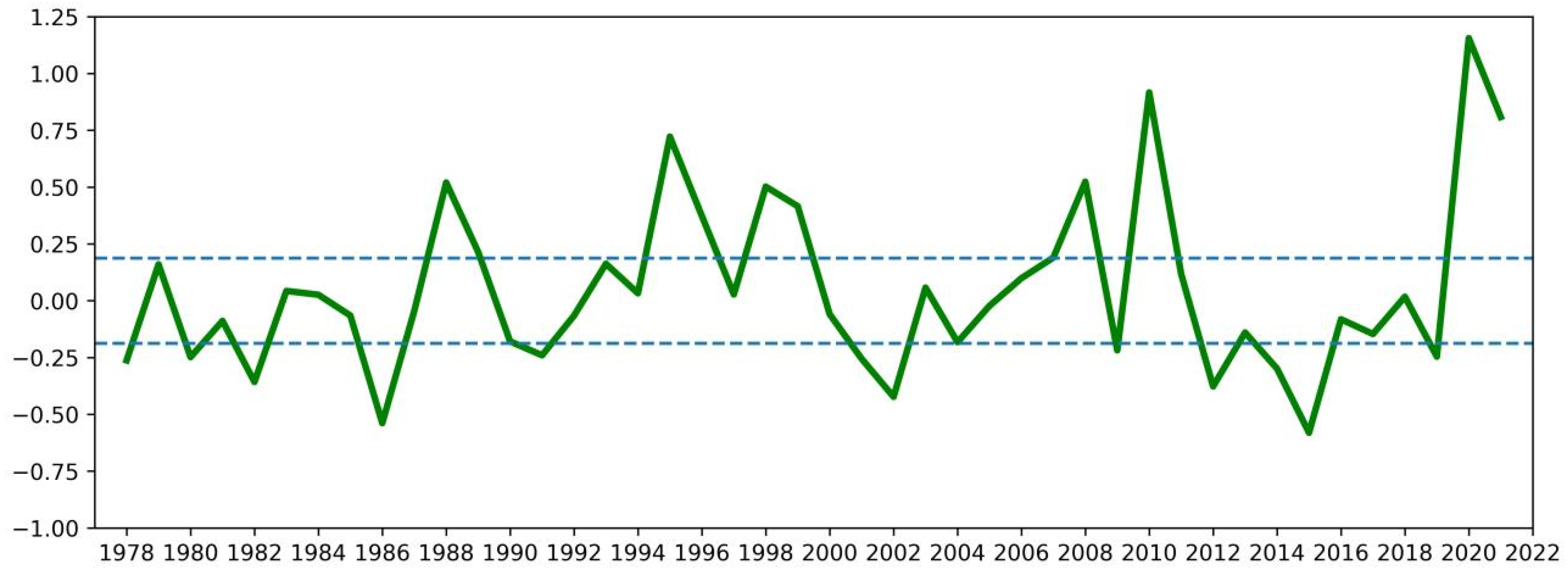
Figure 2.
May–November composite MJO indices from the CPC: (a) I high-value years; (b) I low-value years; (c) differences in composite MJO indices from the CPC between I high- and low-value years (contour). The shaded area indicates that the value is statistically significant at the 95% confidence level.
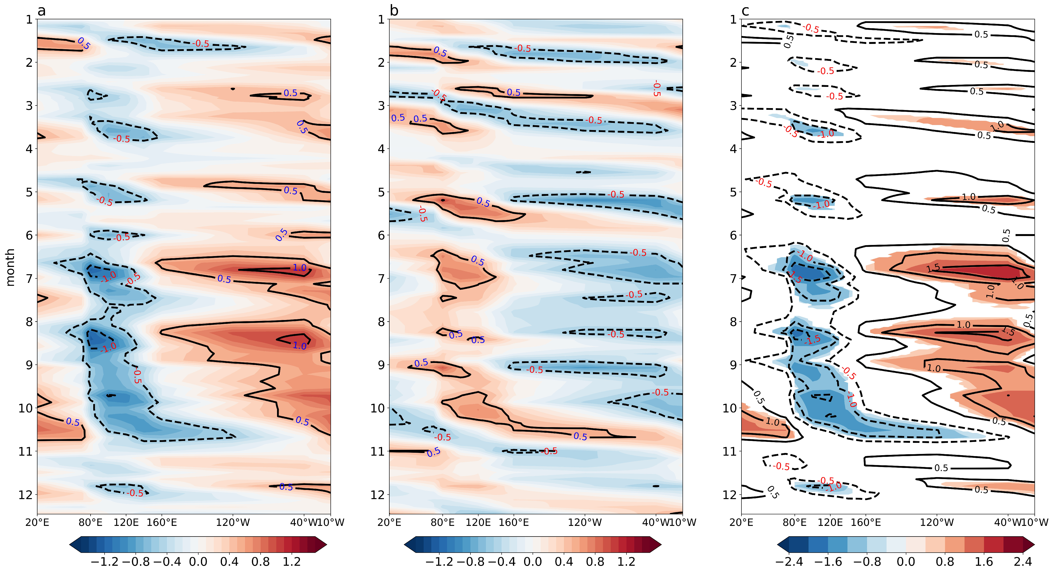
Figure 3.
Annual frequency of TYs in I high- (a) and low-value years (b). The blue line represents the average value of TY frequency.
Figure 3.
Annual frequency of TYs in I high- (a) and low-value years (b). The blue line represents the average value of TY frequency.
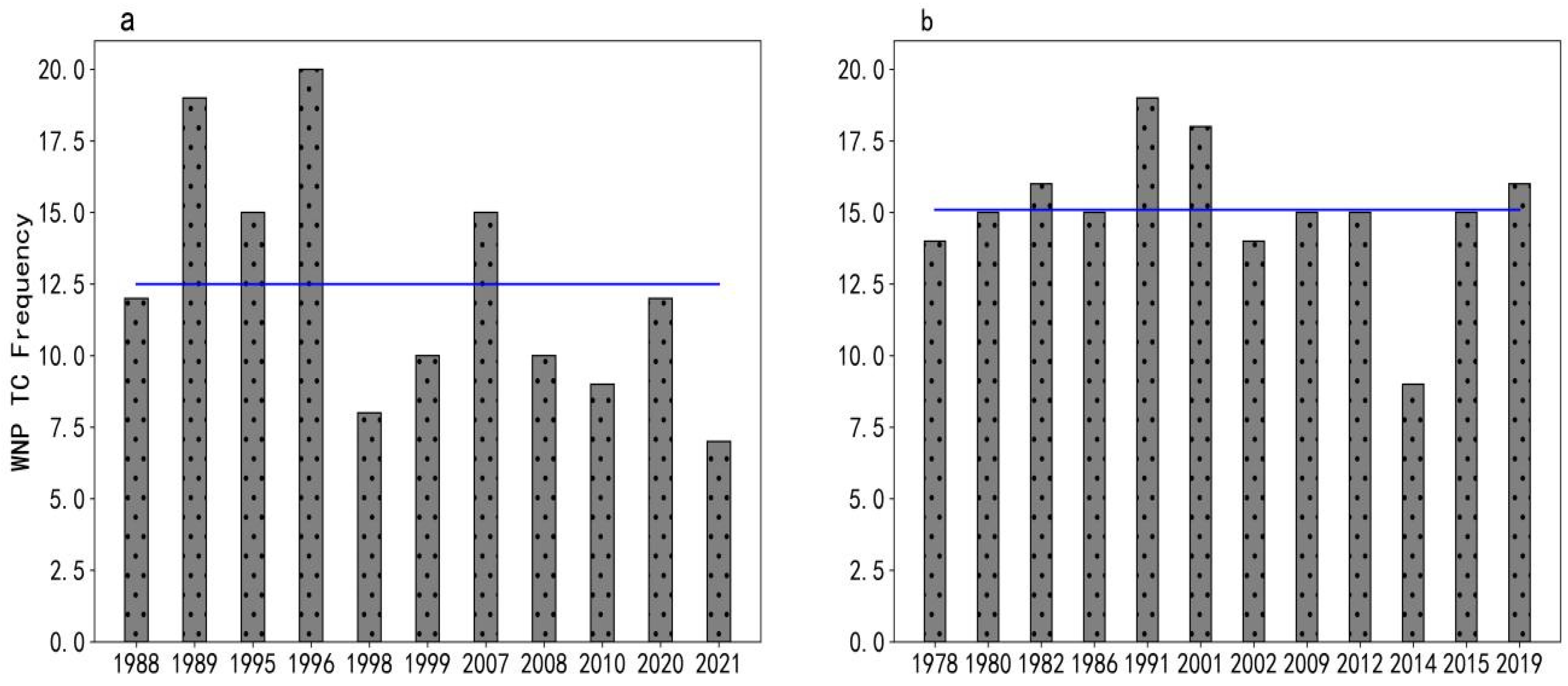
Figure 4.
Spatial distribution of TY generation points for I high- and low-value years. The blue dots represent the TYs for I high-value years, and the orange triangles represent TYs for the I low-value years.
Figure 4.
Spatial distribution of TY generation points for I high- and low-value years. The blue dots represent the TYs for I high-value years, and the orange triangles represent TYs for the I low-value years.
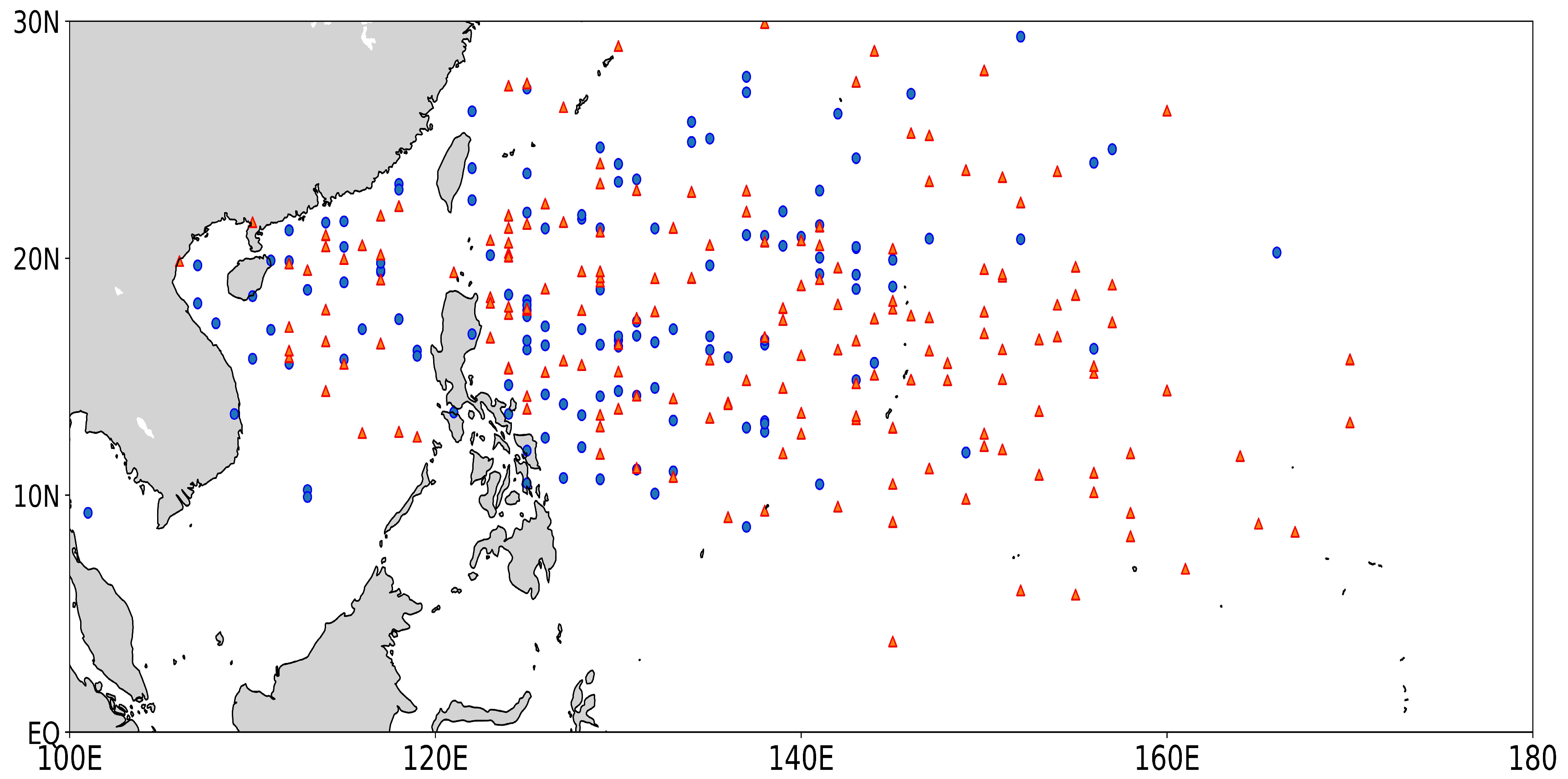
Figure 5.
Composite SST (shaded, units: °C) from May to November for I high- (a) and low-value years (b). The black dashed lines represent the 28.5 °C and 29.5 °C isotherms.
Figure 5.
Composite SST (shaded, units: °C) from May to November for I high- (a) and low-value years (b). The black dashed lines represent the 28.5 °C and 29.5 °C isotherms.
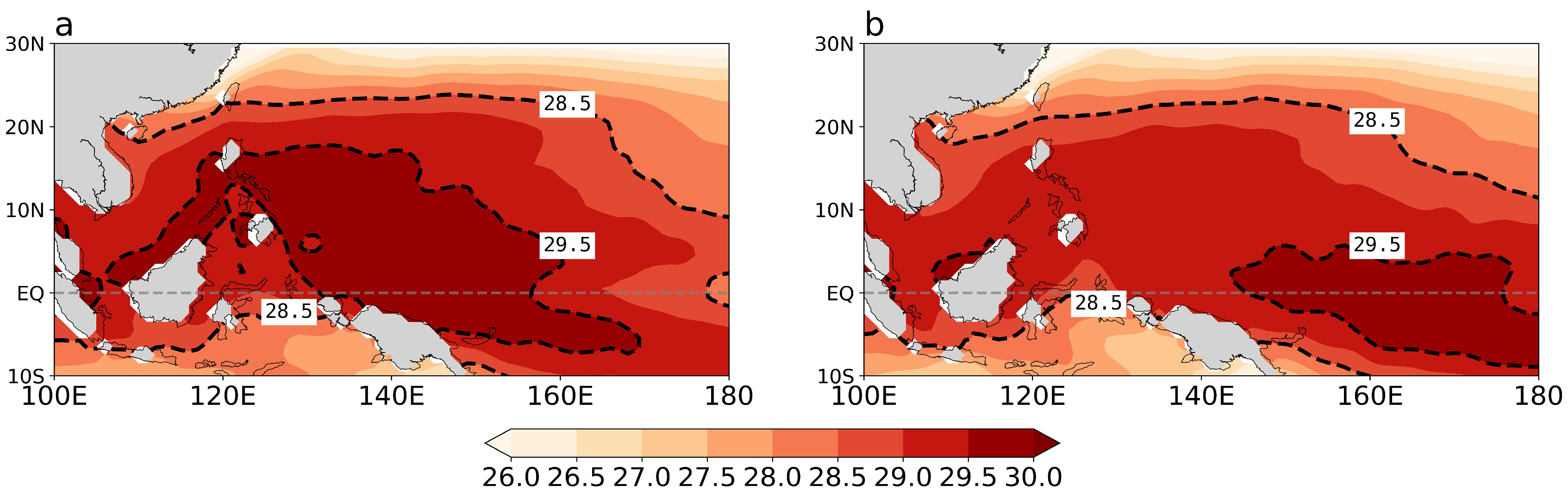
Figure 6.
Locations of 850 hPa composite streamlines and TY (blue dot) generation between May and November for I high- (a) and low-value years (b).
Figure 6.
Locations of 850 hPa composite streamlines and TY (blue dot) generation between May and November for I high- (a) and low-value years (b).

Figure 7.
The anomaly of the composite vertical velocity between 5° N and 15° N for I high- (a) and low-value (b) years (shading, units: Pascal s−1); (c) the differences in the composite vertical velocity between 5° N and 15° N for I high- and low-value years (shading, units: Pascal s−1). The arrows indicate zonal velocities (units: m s−1) and vertical velocities (units: 100 Pascal s−1). These results are statistically significant at the 90% confidence level, as shown by the arrow areas.
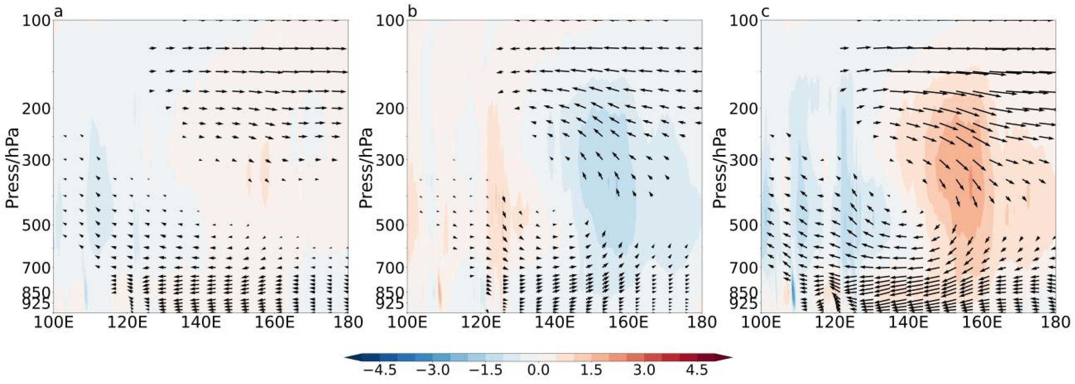
Figure 8.
Differences in composite wind (vector, units: m s−1) and divergence (shading, units: 10−6 s−1) after 30–60-day filtering for (a) 850 hPa and (b) 200 hPa. The arrow areas and the spotted areas are statistically significant at the 95% confidence level.
Figure 8.
Differences in composite wind (vector, units: m s−1) and divergence (shading, units: 10−6 s−1) after 30–60-day filtering for (a) 850 hPa and (b) 200 hPa. The arrow areas and the spotted areas are statistically significant at the 95% confidence level.
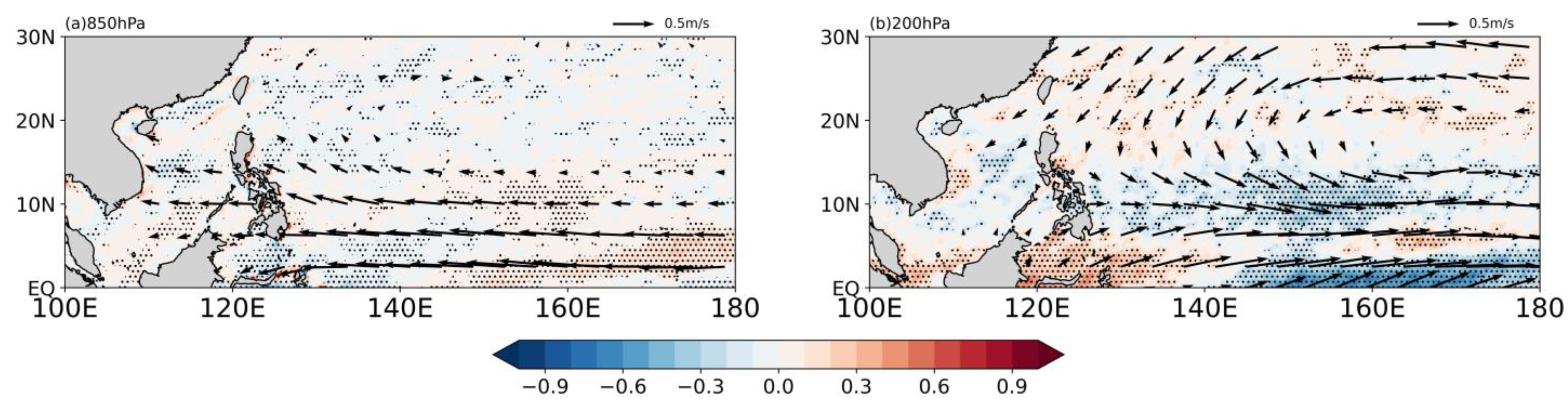
Figure 9.
The differences in composite 850 hPa relative vorticity (shading, unit: 10−6 m s−1) after 30–60-day filtering for I high- and low-value years. The spotted area indicates that the value is statistically significant at the 95% confidence level.
Figure 9.
The differences in composite 850 hPa relative vorticity (shading, unit: 10−6 m s−1) after 30–60-day filtering for I high- and low-value years. The spotted area indicates that the value is statistically significant at the 95% confidence level.
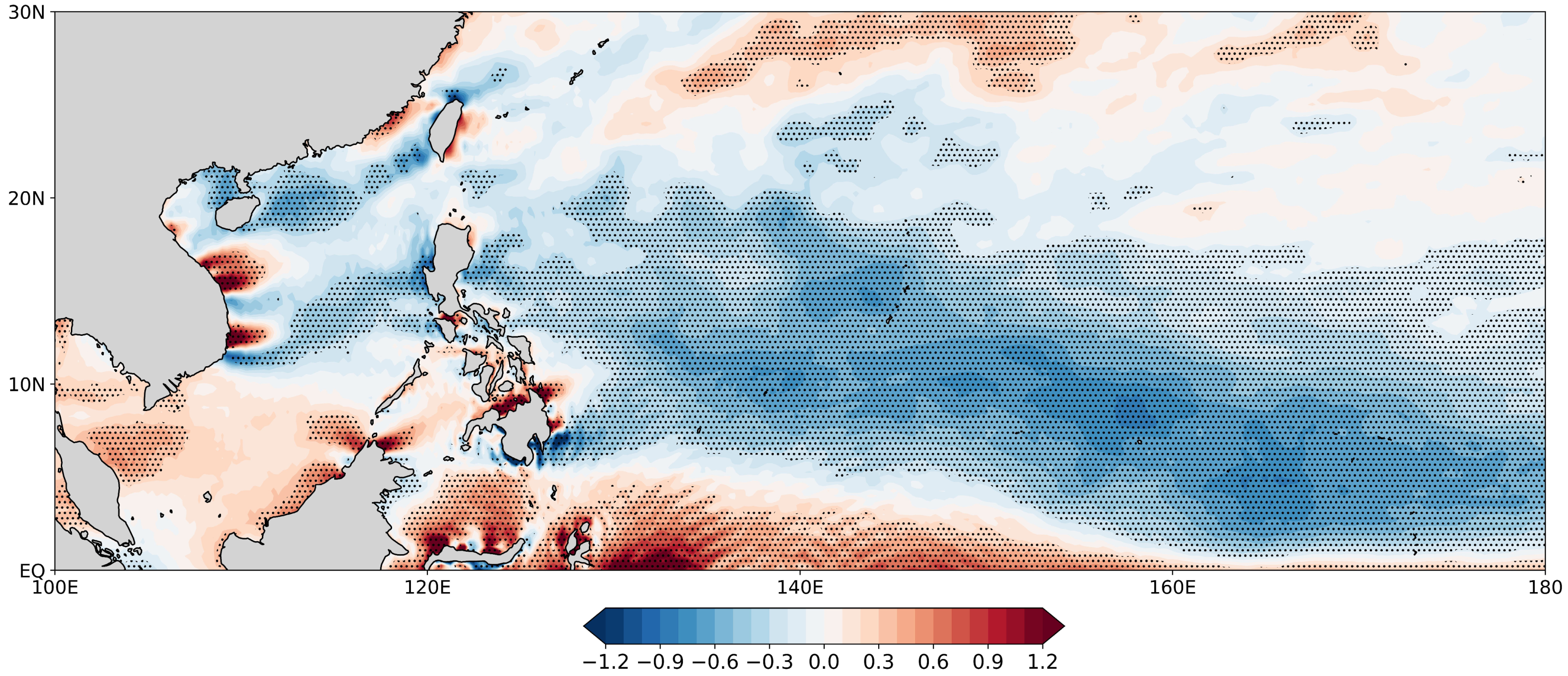
Figure 10.
The differences in composite vertical wind shear (shading, 200-hPa minus 850-hPa, unit: m s−1) after 30–60-day filtering for I high- and low-value years. The shaded area indicates that the value is statistically significant at the 95% confidence level.
Figure 10.
The differences in composite vertical wind shear (shading, 200-hPa minus 850-hPa, unit: m s−1) after 30–60-day filtering for I high- and low-value years. The shaded area indicates that the value is statistically significant at the 95% confidence level.

Figure 11.
The differences in composite 500 hPa relative humidity (shading, unit: %) after 30–60-day filtering for I high- and low-value years. The spotted area indicates that the value is statistically significant at the 90% confidence level.
Figure 11.
The differences in composite 500 hPa relative humidity (shading, unit: %) after 30–60-day filtering for I high- and low-value years. The spotted area indicates that the value is statistically significant at the 90% confidence level.
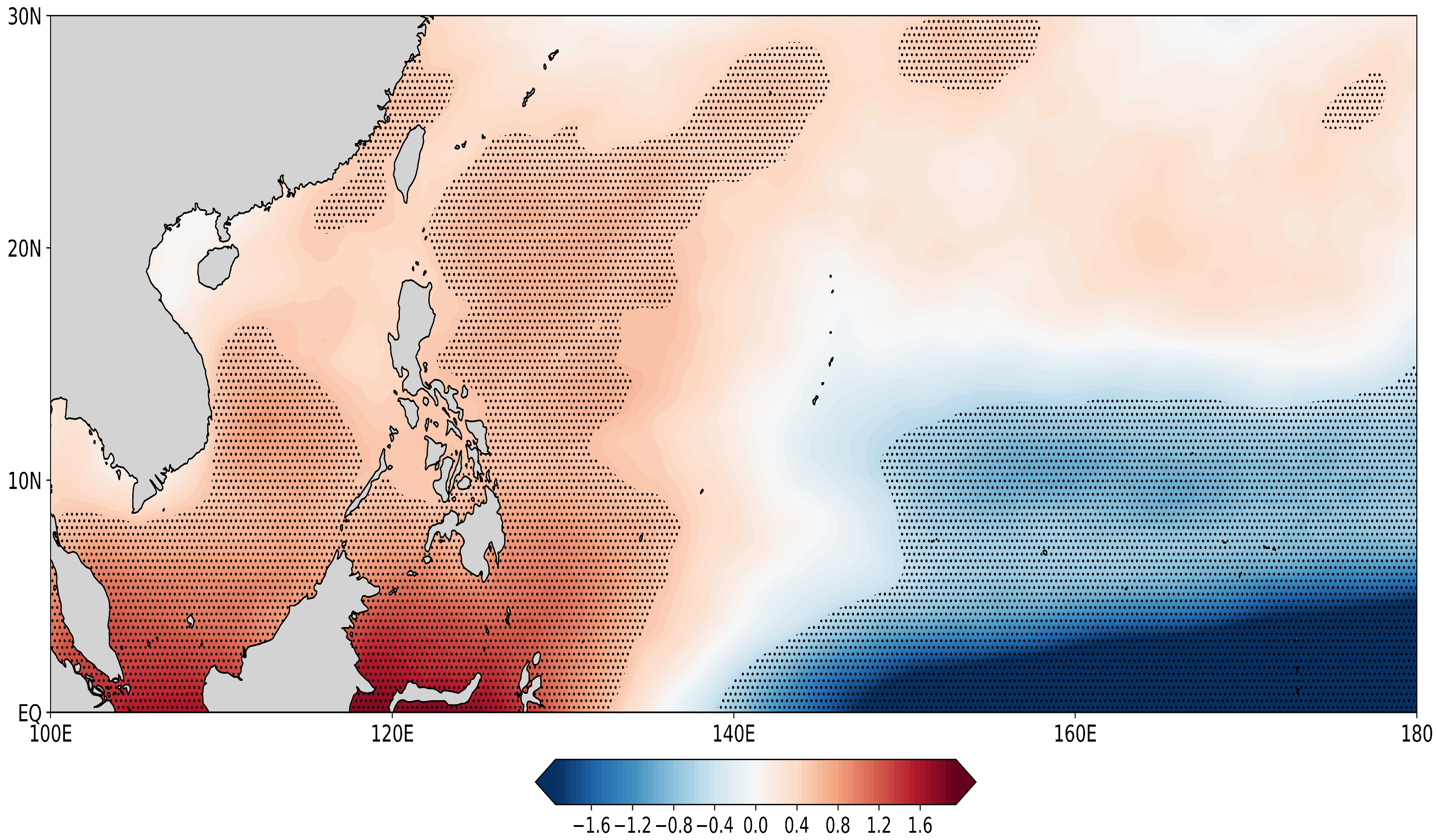
Figure 12.
Physical mechanisms of interannual variation in the generation of TYs affected by I high-value years. The black arrow circles indicate cyclonic circulation (anticyclonic circulation). The solid black lines indicate monsoon troughs. The black dashed lines indicate trough lines. The blue arrows indicate zonal circulation at 5°–15° N. The white arrows indicate winds. The red symbols indicate TYs. The orange areas indicate MJO stagnation. The yellow areas indicate positive vertical wind shear. The green areas indicate positive relative humidity. The purple areas indicate negative relative vorticity. The red areas represent warm pools.

Table 1.
Years with high and low values (I).
| I High-Value Years (11a) | I Low-Value Years (12a) |
| 1988, 1989, 1995, 1996, 1998, 1999, 2007, 2008, 2010, 2020, 2021 | 1978, 1980, 1982, 1986, 1991, 2001, 2002, 2009, 2012, 2014, 2015, 2019 |
Table 2.
Total number of TYs in different longitude ranges for the I high- and low-value years.
| The I High-Value Years | The I Low-Value Years | |
| 100° E–140° E | 106 (77% of the total) | 101 (56% of the total) |
| 140° E–180° E | 31 (23% of the total) | 80 (44% of the total) |
| Total | 137 | 181 |
Disclaimer/Publisher’s Note: The statements, opinions and data contained in all publications are solely those of the individual author(s) and contributor(s) and not of MDPI and/or the editor(s). MDPI and/or the editor(s) disclaim responsibility for any injury to people or property resulting from any ideas, methods, instructions or products referred to in the content. |
© 2024 by the authors. Licensee MDPI, Basel, Switzerland. This article is an open access article distributed under the terms and conditions of the Creative Commons Attribution (CC BY) license (https://creativecommons.org/licenses/by/4.0/).
Share and Cite
MDPI and ACS Style
Lin, C.-q.; Fan, L.-l.; Chen, X.-z.; Li, J.-H.; Xu, J.-j. Modulation of the Madden–Julian Oscillation Center Stagnation on Typhoon Genesis over the Western North Pacific. Atmosphere 2024, 15, 373. https://doi.org/10.3390/atmos15030373
AMA Style
Lin C-q, Fan L-l, Chen X-z, Li J-H, Xu J-j. Modulation of the Madden–Julian Oscillation Center Stagnation on Typhoon Genesis over the Western North Pacific. Atmosphere. 2024; 15(3):373. https://doi.org/10.3390/atmos15030373
Chicago/Turabian StyleLin, Chun-qiao, Ling-li Fan, Xu-zhe Chen, Jia-Hao Li, and Jian-jun Xu. 2024. "Modulation of the Madden–Julian Oscillation Center Stagnation on Typhoon Genesis over the Western North Pacific" Atmosphere 15, no. 3: 373. https://doi.org/10.3390/atmos15030373
Note that from the first issue of 2016, this journal uses article numbers instead of page numbers. See further details here.