Article

The Impact of Vertical Eddy Diffusivity Changes in the CMAQ Model on PM2.5 Concentration Variations in Northeast Asia: Focusing on the Seoul Metropolitan Area

Air Quality Forecasting Center, National Institute of Environmental Research, Incheon 22689, Republic of Korea
*
Author to whom correspondence should be addressed.
Atmosphere 2024, 15(3), 376; https://doi.org/10.3390/atmos15030376
Submission received: 28 February 2024 / Revised: 15 March 2024 / Accepted: 17 March 2024 / Published: 19 March 2024
(This article belongs to the Special Issue Novel Insights into Air Pollution over East Asia)

Abstract

:
The vertical eddy diffusion process plays a crucial role in PM2.5 prediction, yet accurately predicting it remains challenging. In the three-dimensional atmospheric chemistry transport model (3-D AQM) CMAQ, a parameter, Kz, is utilized, and it is known that PM2.5 prediction tendencies vary according to the floor value of this parameter (Kzmin). This study aims to examine prediction characteristics according to Kzmin values, targeting days exceeding the Korean air quality standards, and to derive appropriate Kzmin values for predicting PM2.5 concentrations in the DJFM Seoul Metropolitan Area (SMA). Kzmin values of 0.01, 0.5, 1.0, and 2.0, based on the model version and land cover, were applied as single values. Initially focusing on December 4th to 12th, 2020, the prediction characteristics were examined during periods of local and inflow influence. Results showed that in both periods, as Kzmin increased, surface concentrations over land decreased while those in the upper atmosphere increased, whereas over the sea, concentrations increased in both layers due to the influence of advection and diffusion without emissions. During the inflow period, the increase in vertically diffused pollutants led to increased inflow concentrations and affected contribution assessments. Long-term evaluations from December 2020 to March 2021 indicated that the prediction performance was superior when Kzmin was set to 0.01, but it was not significant for the upwind region (China). To improve trans-boundary effects, optimal values were applied differentially by region (0.01 for Korea, 1.0 for China, and 0.01 for other regions), resulting in significantly improved prediction performance with an R of 0.78, IOA of 0.88, and NMB of 0.7%. These findings highlight the significant influence of Kzmin values on winter season PM2.5 prediction tendencies in the SMA and underscore the need for considering differential application of optimal values by region when interpreting research and making policy decisions.

1. Introduction

The International Agency for Research on Cancer (IARC), under the auspices of the World Health Organization (WHO), classified fine particulate matter (PM2.5) as a Group 1 carcinogen in October 2013 [1]. Among these, PM2.5, with its larger surface area, tends to adsorb more harmful substances. Additionally, due to its small particle size, PM2.5 can easily penetrate human organs, posing adverse health effects and leading to socio-economic damage through associated effects [2,3,4,5]. In 2020, South Korea had the highest PM2.5 concentration among the Organization for Economic Cooperation and Development (OECD) member countries, with a concentration of 25.9 µg/m3 [6]. The OECD has forecasted that without intervention measures, South Korea’s premature mortality rate and economic losses would be the highest among member countries by 2060 [7]. Consequently, the Ministry of Environment (ME) has implemented emission reduction policies and measures for minimizing PM2.5-related damages, including fine dust forecasts. Reliable predictive information is crucial for the successful implementation of these efforts.
Various three-dimensional atmospheric chemistry transport models, such as Community Multi-scale Air Quality (CMAQ), Weather Research and Forecasting with Chemistry (WRF-Chem), Regional-Scale Modeling (RSM), and the Comprehensive Air Quality Model with Extensions (CAMx), are utilized for PM2.5 prediction [8,9,10,11,12]. Among these, the CMAQ model, while challenging to interpret due to its complex and diverse input parameters, offers advantages in considering complex interactions among pollutants through detailed physical and chemical process modeling. Moreover, it undergoes continuous development by various researchers as a community model. Given these advantages, the ME employs the CMAQ model in various fields, ranging from simulation of air quality improvement policies to air quality forecasting and environmental monitoring.
The CMAQ model calculates PM2.5 concentrations through various and complex processes, including meteorology, emissions, dry and wet deposition, chemical reactions, and vertical and horizontal advection and diffusion. Among them, vertical diffusion directly influences the vertical distribution of PM2.5 concentration by dispersing pollutants (including those emitted from sources) suspended in the atmosphere [13,14,15]. However, vertical diffusion is difficult to predict accurately due to turbulent and non-stationary characteristics. To calculate this, the CMAQ model utilizes a parameter called the vertical turbulent diffusion coefficient (Kz). Kz values range from hundreds of m2/s on days with strong thermal buoyancy to below 1.0 m2/s during nighttime, when the planetary boundary layer (PBL) height decreases [16]. The CMAQ model applies a minimum eddy diffusivity (Kzmin) to prevent Kz from falling below 0.
Li and Rappenglueck compared experiments using the KZMIN option of the CMAQ model with a fixed Kzmin of 1.0 m2/s and varied values ranging from 0.01 to 1.0 m2/s depending on land cover and found that nighttime ozone bias in the Texas region decreased by up to 31% [17]. Furthermore, Castellanos et al. and Jin et al. analyzed ozone predictability when the Kzmin of the CMAQ model was reduced from 0.5 m2/s to 0.1 m2/s [18,19]. According to Castellanos et al., the CMAQ model overestimated nighttime ozone in both urban and rural areas in the eastern United States, and the ozone prediction bias decreased when Kzmin was 0.1 m2/s [18]. Similarly, Jin et al. identified that when Kzmin was 0.1 m2/s, the CMAQ model simulated the nighttime and early morning ozone concentrations in inland areas as being approximately 10 ppb lower [19]. Accordingly, numerous previous studies have been conducted as the appropriate use of Kzmin values is a crucial factor in predicting pollutant concentrations [20,21,22,23,24]. However, most previous studies have focused on ozone, showing improved ozone predictability with reduced Kzmin values. According to Kim et al., the use of reduced Kzmin values resulted in overestimation of surface PM2.5 concentrations in Northeast Asia, showing contrasting results to ozone [25]. Despite varying sensitivity to Kzmin values depending on pollutants, research on PM2.5 is insufficient. Additionally, existing studies have primarily considered specific episodes and local impacts, highlighting the need for research tailored to the geographic characteristics of South Korea, which is influenced by pollutants transported from neighboring countries [26,27].
Therefore, we aim to analyze the predictive performance of the CMAQ model for PM2.5 in the Seoul Metropolitan Area (SMA) during the winter season. The analysis is to be conducted based on different Kzmin values, considering both local and long-range transport influences in order to derive appropriate Kzmin values. Specifically, Section 3.1 analyzes the impact of Kzmin variations on local PM2.5 concentrations and concentrations from foreign sources for high-concentration cases exceeding the Korean air quality standard (daily average concentration of 35 µg/m3), while Section 3.2 determines suitable Kzmin values for winter season concentration predictions through long-term analysis.

2. Methodology

2.1. Model Configuration

We conducted PM2.5 concentration predictions using the CMAQ v5.0.2 model. The Meteorology Chemistry Interface Processor (MCIP) v4.2 was employed to recalibrate the results from the Weather Research and Forecasting model (WRF) v3.8.1 to match the CMAQ grid system. Emission input data consisted of both natural emissions estimated using the Model of Emissions of Gases and Aerosols from Nature (MEGAN) v2.0.4 and anthropogenic emissions calculated using Sparse Matrix Operator Kernel Emission (SMOKE) v3.1, which were combined. For this, the European Centre for Medium-Range Weather Forecasts Reanalysis version 5 (ECMWF-ERA5) was utilized as the initial and boundary conditions for WRF, and foreign anthropogenic emissions were based on the Korea US Air Quality Study (KORUS-AQ) v5 [28], while domestic anthropogenic emissions were sourced from the Clean Air Policy Support System (CAPSS) 2016 [29]. The modeling domain was set up to analyze the influence of pollutants transported from surrounding countries to the SMA, with the mother domain (D1) covering Northeast Asia, including Russia, Mongolia, China, and Japan, and the smaller domain (D2) encompassing the Korean Peninsula, including the SMA (Figure 1). The model was run with one-way nesting over a total of 15 layers (Top: approximately 20 km, surface: approximately 0.03 km). Detailed domain information and the model’s physical and chemical options are described in Table 1.

2.2. Experimental Design

CMAQ calculates vertical mixing due to turbulence using K-theory and Bulk Richardson number [30]. The floor value of Kz in the CMAQ model, represented by Kzmin, was previously fixed at a single value (1.0 m2/s). However, since version 4.6, CMAQ has utilized the KZMIN option, which incorporates the effect of land cover, as described by the following equation.
K z m i n = K Z L + K Z U K Z L U F R A C
U F R A C = 0.01 P U R B
Here, KZL and KZU were previously set at constant values of 0.5 and 2.0 before CMAQ v5, and 0.01 and 1.0 afterwards, while UFRAC (Urban Fraction) represents the proportion of urban land cover, calculated using the urban fraction PURB (ranging from 0% to 100%) as shown in Equation (2). Consequently, Kzmin in CMAQ ranges from 0.01 to 2.0 depending on the model version and UFRAC. Therefore, we conducted experiments using single values for the upper and lower limits of Kzmin (0.01, 0.5, 1.0, 2.0) to predict PM2.5 concentrations in the Base experiment (hereafter referred to as B) and to analyze net concentrations from abroad by zeroing out domestic emissions in the Zero-out experiment (hereafter referred to as Z). These experiments were named B0.01, B0.5, B1.0, B2.0, Z0.01, Z0.5, Z1.0, and Z2.0, according to the applied Kzmin values.

2.3. Target Cases and Regions

In South Korea, PM2.5 concentrations gradually decrease after March, reaching their lowest levels from July to September, and then begin to rise again from October, leading to frequent exceedances of the Korean air quality standards from December to the following March. Among these, the SMA serves as a major hub where approximately 50% of the Korean population resides. It is characterized by various emission sources (such as roads, residential areas, industrial facilities, and industrial complexes) and is susceptible to both local and long-range transport influences due to its geographical proximity to neighboring countries, including China [31,32]. Particularly during certain periods, foreign long-range transport influences dominate, necessitating the consideration of changes in foreign PM2.5 concentrations in the SMA based on Kzmin values [33,34]. Therefore, we analyzed the PM2.5 prediction performance based on Kzmin values in the SMA from December 2020 to March 2021. Initially, we examined the predictive characteristics based on Kzmin values during the period from 4 December to 12 December 2020, when both local and long-range transport influences were occurring, and subsequently derived the most optimal Kzmin values through a long-term evaluation (four months). In order to understand the impact of long-range transport, we included the Northeast (NE), Northcentral (NC), Southeast (SE), and Southcentral (SC) regions of China, which are the major source regions of air masses entering the SMA during the winter, as well as the Yellow Sea (YS) area, in the analysis target areas [35] (Figure 1).

2.4. Analysis Methodology

In South Korea, the ME operates the Air Quality Monitoring System (AQMS) for various purposes. The AQMS includes urban air monitoring networks, rural air monitoring networks, national background monitoring networks, roadside monitoring networks, etc. Among these, we utilized the hourly data from urban air monitoring networks, which represent the average air quality concentrations in urban areas. Data from a total of 473 monitoring stations were used in the study, with 154 stations corresponding to the SMA. Data from the Baengnyeongdo station, which represents the Yellow Sea (YS), were used as a representative observation point for YS. The national background monitoring network is situated in relatively independent locations from domestic emissions, making it suitable for assessing national background concentrations and long-range transport of pollutants from overseas sources. Additionally, to evaluate the predictability of source regions, hourly data from 900 monitoring stations provided by an air quality website (https://air-quality.com (accessed on 15 March 2024)) were utilized.
The validation of model performance employed metrics such as normalized mean bias (NMB), index of agreement (IOA), and coefficient of correlation (R), which are indicators for assessing the tendency of overestimation or underestimation, consistency with estimates, and correlation, respectively. Generally, when NMB approaches 0, and both IOA and R approach 1, it indicates that the model effectively simulates actual phenomena. Specifically for PM2.5, a model’s performance is considered good when NMB falls within ±30%, IOA is ≥0.5, and R is ≥0.4. Furthermore, a model’s performance is deemed excellent when NMB is within ±10% and R is ≥0.7 [36,37,38].
Subsequently, we analyzed the variations in prediction characteristics (spatiotemporal distribution, backward trajectory analysis, domestic and foreign contributions, etc.) as Kzmin increased. This was performed using the B0.01 experiment, which represents the scenario with the most suppressed vertical diffusion, as a reference. For backward trajectory analysis, we employed the Hybrid Single-Particle Lagrangian Integrated Trajectory model (HYSPLIT), developed by the National Oceanic and Atmospheric Administration (NOAA). To estimate domestic and foreign contributions, we utilized the brute force method (BFM) (Equations (3) and (4)), widely employed by agencies such as the United States Environmental Protection Agency (EPA) and the European Monitoring and Evaluation Program (EMEP).
C D o m e s t i c ( μ g / m 3 ) = C B a s e C Δ ε × 100 ε
R F o r e i g n ( % ) = C B a s e C D o m e s t i c C B a s e × 100
Here, C B a s e , C Δ ε , and C D o m e s t i c represent the concentrations in the B experiment, Z experiment, and domestic contributions, respectively, and R F o r e i g n denotes the foreign contribution. In this study, 100 ε equaling one, domestic contribution is defined as the difference between the B and Z experiments, whereas foreign contribution is defined as the ratio of Z to B experiments ( C Z C B ).

3. Results and Discussion
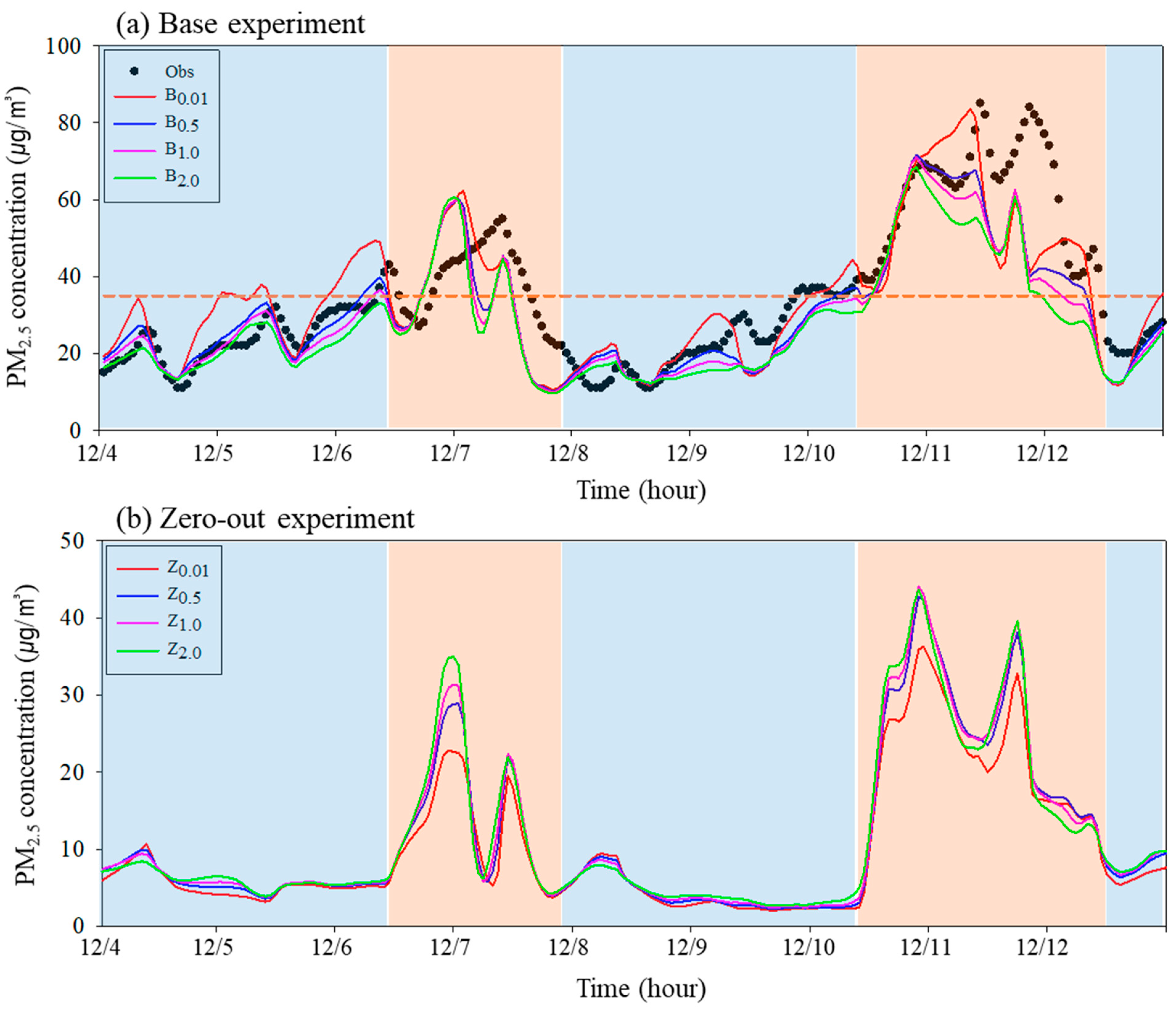
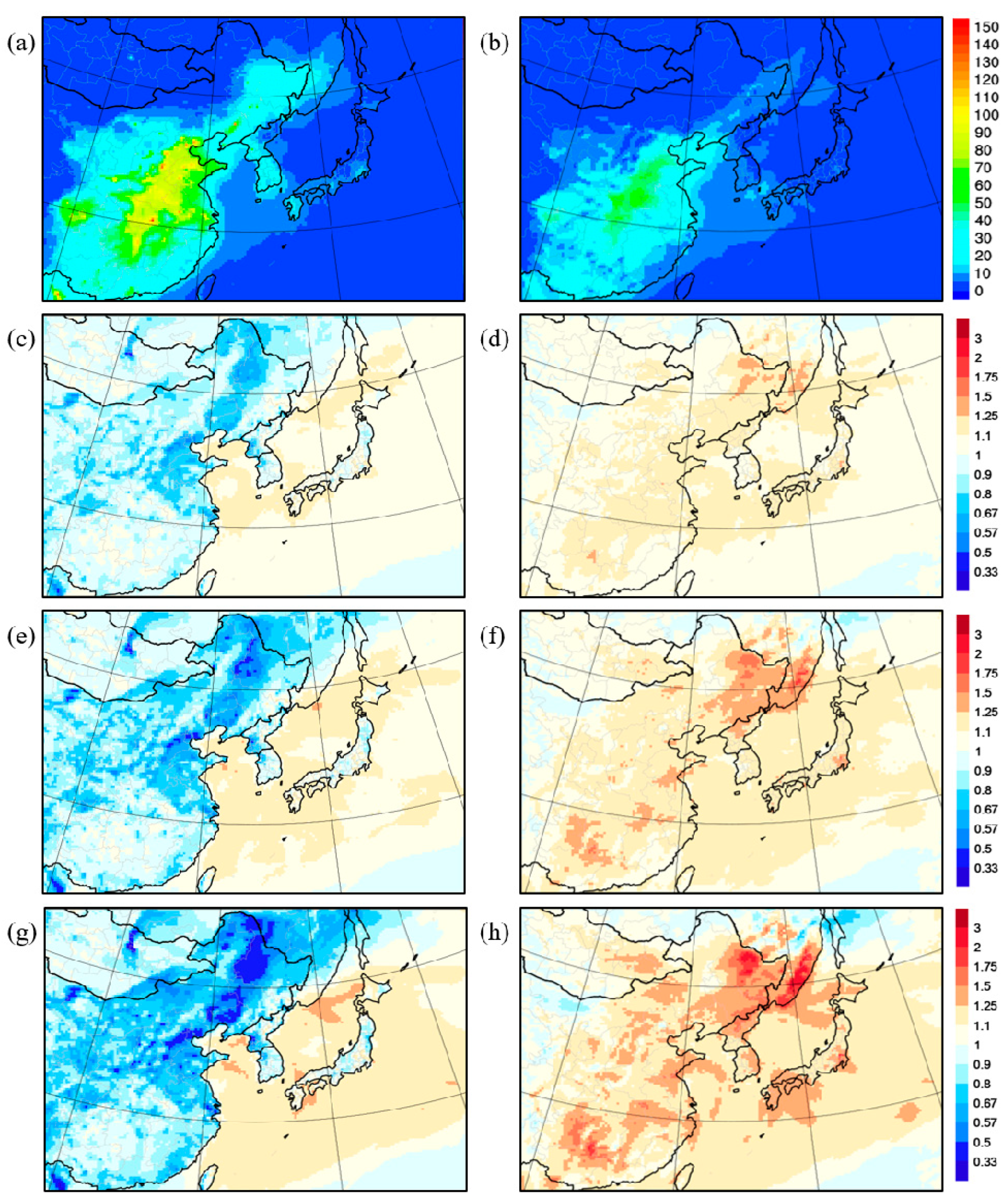
3.1. Case Analysis

Statistical validation confirmed that the results of the B experiment used in the study exhibited significant performance (good model) across the board. The experiments demonstrated R and IOA values in the range of 0.8 to 0.9, indicating that they adequately simulated the variability of observations. While an increase in Kzmin values showed an associated increase in errors, the NMB remained within −30%. These findings suggest that the numerical model used in this study sufficiently simulate observations, and it is apparent that Kzmin values exert a greater influence on error variation than variability.
Figure 2 depicts the PM2.5 concentration time series for the B and Z experiments during the case period. Here, the point of sharp increase in concentration in the Z experiment is defined as the inflow period, while the point of decrease is defined as the outflow period. The case period is divided into inflow period (orange shading) and local influence period (blue shading), with the inflow period further divided into inflow period one (6 December, 09LST to 7 December 15LST) and inflow period two (10 December, 09LST to 12 December, 09LST).

3.1.1. Local Influence Period

Figure 3 presents the distribution of average PM2.5 concentrations at lower (approximately 30 m) and upper (approximately 850 m) levels during the local impact period, showing the results of the B0.01 experiment Figure 3a,b and the predicted concentration ratios of each experiment Figure 3c–h. Initially, the B0.01 experiment predicted high concentrations spanning both the lower and upper levels, with a focus on the NC and SC areas of China. As Kzmin increased, the rate of concentration change in the NC and NE areas increased, with the highest change observed in the NC area. Consequently, compared to B0.01, the surface concentration was under-predicted by 0.5–0.6 times, while the upper-level concentration was over-predicted by 1.1–1.2 times in the NC area. Considering the over-prediction of PM2.5 concentrations by B0.01 compared to observed values in the NC area, it can be inferred that the tendency to over-predict surface concentrations decreases as Kzmin increases. Additionally, as Kzmin increased, there was a tendency for surface concentrations to decrease over land and increase in the upper levels. Conversely, over the ocean, concentrations increased in both lower and upper levels. The decrease in surface concentrations over land can be attributed to differences in diffusion intensity and chemical reaction timing according to Kzmin. As diffusion intensity increases, the reaction time between pollutants distributed on the surface decreases, leading to a decrease in PM2.5 concentrations compared to B0.01 [14]. Conversely, in the upper levels, the increased amount of pollutants moving from the lower levels resulted in increased concentrations. The area of concentration that increased in the upper levels, influenced by the airflow, appeared to be wider to the east compared to the area of concentration that decreased in the lower levels.
As shown in the previous results, the variation in PM2.5 predicted concentrations due to Kzmin also influenced the estimation of contributions using the BFM, which relies on predicted concentrations. Figure 4 presents the contribution analysis results, showing that during the local impact period in the SMA area, the domestic contribution decreased as Kzmin increased. This can be observed from the Z experiment results in Figure 2, where there was little difference in the inter-experimental foreign contribution (4.9–5.5 μg/m3), but the domestic contribution varied between 20.9, 16.6, 15.2, and 13.7 μg/m3 among experiments, representing a maximum difference of 34.3% between experiments. This suggests that despite no changes in external conditions (such as inflow patterns or emissions), the decrease in domestic contribution occurred due to the variation in internal model dynamics.

3.1.2. Long-Range Transport Influence Period

Figure 5 depicts the results of backward trajectory analysis conducted for the daytime periods (point 1: 15:00 LST on the 6th, point 2: 15:00 LST on the 10th) during the inflow period, where pollutants transported by vertical diffusion influence the surface. Figure 6 shows the vertical cross-sections of PM2.5 concentrations from the Z experiment at various time points, considering the trajectories of airflow movement. During the first inflow period on December 6th at 15:00 LST, the airflow entering the upper layer of the SMA (at 640 m) passed through the NC area and crossed the YS. While the altitude of the airflow gradually decreased over land, it maintained a consistent altitude when passing over the sea. During the second inflow period on December 10th at 15:00 LST, the airflow entering the upper layer of the SMA (at 1000 m) formed a V-shape as it moved through the SC area before crossing the YS. Unlike the first inflow period, the airflow during this period maintained a relatively consistent altitude throughout its movement.
We compared and analyzed the wind vectors of the B0.01 experiment with the results from HYSPLIT, confirming that they simulate the influx of pollutants in a similar manner (Figure 6a,b). As the airflow passed over land, the vertical distribution of PM2.5 concentrations exhibited a peak near the surface due to the influence of emitted pollutants, decreasing as it moved upward. During the daytime, strong vertical diffusion led to a relatively uniform distribution of concentrations between the lower and upper layers, whereas during the nighttime, diffusion was suppressed, resulting in a more pronounced gradient between the lower and upper layers. In contrast, when the airflow passed over the sea (YS), there was minimal influence from emissions, with the concentration gradient being less pronounced due to advection and diffusion. Unlike over land, there were sections where concentrations were higher in the upper layer than in the lower layer. This indicates that pollutants were transported to the upper layer during both the first and second inflow periods, with vertical diffusion likely impacting the surface during daylight hours.
The vertical concentration changes with respect to Kzmin were similar to the results presented in Figure 3. Overall, as Kzmin increased, there was a significant decrease in concentrations near the surface over land, accompanied by an increase in concentrations at higher altitudes. The time points showing the largest differences compared to the B0.01 experiment were identified as 5 December at 00LST and 9 December at 09LST, where increasing Kzmin values resulted in surface concentrations being predicted as much as 81.1 µg/m3 and 84.3 µg/m3 lower, while upper-level concentrations (at 850 m and 300 m) were predicted as much as 4.8 µg/m3 and 40.9 µg/m3 higher, respectively. When integrating the results from HYSPLIT with the vertical concentration distribution, it was observed that the concentration of pollutants transported into SMA increased proportionally with Kzmin values. The most significant difference was observed at 7 December at 00LST, where surface concentrations increased by 6.2 µg/m3 and 8.7 µg/m3, respectively, compared to the B0.01 experiment.
During the periods of inflow influence, the domestic contribution concentrations for each experiment were 30.4 µg/m3, 24.7 µg/m3, 22.5 µg/m3, and 20.0 µg/m3, while the foreign contribution concentrations were 8.6 µg/m3, 21.1 µg/m3, 21.5 µg/m3, and 21.6 µg/m3, respectively, showing a decrease in domestic contribution concentrations and an increase in foreign contribution concentrations as Kzmin values increased (refer to Figure 4). As a result, compared to the B0.01 experiment, the foreign contribution was higher by a minimum of 8.2 percentage points (p) and a maximum of 14.0 percentage points (p), with respect to the total concentration. It is important to note that due to the non-linear relationship between concentration and emissions, the actual foreign contribution is expected to be even higher.
Indeed, Kzmin not only affects the prediction of PM2.5 concentrations, but also influences the estimation of contributions. Therefore, setting appropriate values for Kzmin is crucial for providing reliable prediction information. In areas like the SMA, which are subject to both local and inflow influences, it is especially important to consider the impact from upwind regions (such as China, Mongolia, etc.) along with local factors. This comprehensive approach ensures a more accurate understanding of air quality dynamics and enables better-informed decision-making for managing air pollution.

3.2. Long-Term Evaluation

Figure 7 shows the performance evaluation results of the B experiments from December 2020 to March 2021. Initially, all B experiments underestimated observations in the SMA area, but they exhibited significant performance with R ranging from 0.7 to 0.8, IOA from 0.8 to 0.9, and NMB from -19% to 0%. Particularly, B0.01 showed the best performance with an R of 0.79, IOA of 0.88, and NMB of −3.6. Regarding upwind areas such as China, B0.5 and B1.0 showed excellent performance, while B2.0 exhibited significant performance. The B0.5, B1.0, and B2.0 experiments also demonstrated significant or excellent performance for the NE, NC, and SC areas. However, only B2.0 showed significant performance in the NE area. B0.01 showed insignificant performance across all areas, with NMB ranging from −11.6% to 63.9%, indicating significant variability in errors and inadequate simulation of observations.
In summary, while B0.01 showed the best predictive performance for the SMA region, B1.0 performed best for China, highlighting significant variability in predictive capabilities based on the applied Kzmin values. Although the predictive performance based on the applied Kzmin values showed less variability for Korea, significant differences were observed for China. Given that B0.01, which exhibited superior predictive performance for the SMA region, did not perform well for China, we conducted a new experiment, termed Bnew, to improve the trans-boundary effects of B0.01. In the Bnew experiment, we applied different optimal Kzmin values for each region. Specifically, we applied a Kzmin value of 0.01 for Korea, 1.0 for China, and 0.01 for other regions such as Mongolia, Russia, and Japan. This approach aimed to optimize predictive performance based on regional characteristics.
As a result, the Bnew experiment showed a significant improvement in predictive performance for China compared to the B0.01 experiment, with NMB improving by up to 50.8 percentage points in the NC area (Table 2). This improvement in predictive characteristics for China in the Bnew experiment closely resembled those of the B1.0 experiment. To assess the impact of the improvement in predictive performance for China on the downwind side, we analyzed the data from the Baengnyeongdo monitoring station, which represents the national background concentration. The Bnew experiment exhibited an R value of 0.56, IOA of 0.70, and NMB of −35.9%, showing some improvement compared to B0.01 (B0.01: R 0.55, IOA 0.66, NMB −43.8%). Figure 8 presents the daily average concentration roses and NMB results for B0.01 and Bnew at the Baengnyeongdo station, categorized by the most frequent wind direction from hourly model-predicted wind data. Relative to B0.01, Bnew simulated higher concentrations, particularly when westerly winds were predicted, resulting in increased frequency of high-concentration events (daily average exceeding 35 µg/m3). For instance, the frequency of events exceeding the 35–50 µg/m3 range increased from zero to three events for westerly winds, from four to seven events for southwesterly winds, and from zero to one event for northwesterly winds. Furthermore, Bnew showed an improvement in NMB for all wind directions compared to B0.01, ranging from a minimum improvement of 0.1 percentage points to a maximum of 4.6 percentage points. Notably, errors were significantly reduced by 4.0 percentage points (from −7.4% to −3.4%) for westerly winds and by 4.6 percentage points (from −13.3% to −8.7%) for southwesterly winds. Overall, by applying a Kzmin value of 1.0 for China, Bnew demonstrated an improved trans-boundary effect compared to B0.01, resulting in excellent predictive performance for the SMA region, with an R value of 0.78, IOA of 0.88, and NMB of 0.7%.

4. Conclusions

In this study, we analyzed the PM2.5 prediction characteristics of the SMA region based on cases exhibiting both local and long-range transport impacts (from December 4 to 12, 2020), and derived the most suitable Kzmin values through long-term evaluation during the winter season (December 2020 to March 2021). Kzmin values of 0.01, 0.5, 1.0, and 2.0 were applied, considering the model version and upper and lower limits based on land cover.
The experiments conducted in this study demonstrated significant performance for both target cases and long-term evaluation during the winter season, with the variation in Kzmin values proving more effective in improving errors than the model’s variability. Specifically, the analysis of case studies revealed that the change in predicted concentrations according to Kzmin varied depending on surface conditions (land or sea). This variation was attributed to the density of emissions sources, where increasing Kzmin led to decreased surface concentrations and increased upper-level concentrations in densely industrialized terrestrial areas. Conversely, in marine areas with relatively few emission sources, only the influences of advection and diffusion occurred, resulting in an increase in both upper and lower-level concentrations. Accordingly, in cases where local influences predominated, surface concentrations in the SMA decreased with increasing Kzmin, while in cases dominated by foreign inflows, the predicted concentration remained similar across experiments as upper-level PM2.5 concentrations increased with increasing Kzmin, leading to increased long-range transport concentrations.
The variation in predicted concentrations according to Kzmin also affected the contribution assessment results using the BFM. Particularly, the variation in contributions from foreign long-range transport periods (domestic: 62.1–48.1%, foreign: 37.9–51.9%) was greater than that during local influence periods (domestic: 71.3–81.2%, foreign: 18.8–28.7%). Hence, appropriate consideration of Kzmin values reflecting the characteristics of inflow regions is crucial, as it affects both local and inflow concentrations.
In the long-term evaluation during the winter season of 2020, applying Kzmin as 0.01 (B0.01) resulted in the highest IOA and R of 0.88 and 0.79, respectively, and a NMB of −3.6% for the SMA. However, for the inflow region of China, the IOA and R ranged from 0.54 to 0.75 and 0.44 to 0.63, respectively, with a NMB range of 16.1 to 63.9%, indicating significant overestimation and insignificant results. To address the trans-boundary effect from China to the SMA, an experiment (BNew) applying Kzmin as 1.0 was performed (the other region applying as 0.01). The BNew experiment exhibited excellent predictive performance for the SMA, with an IOA, R, and NMB of 0.88, 0.78, and 0.7%, respectively.
This underscores the importance of using appropriate Kzmin values as a crucial factor influencing predictive performance when high concentrations occur. However, as demonstrated in this study, applying a single value may lead to different predictive performances depending on the region. Therefore, it is essential to apply different optimal values based on region, especially in cases of high concentrations due to long-range transport, where applying Kzmin values determines inflow concentrations, thus necessitating their mandatory application for improving trans-boundary effects. Further studies considering the characteristics of windward regions (Mongolia, Russia, Japan, etc.) and inflow current patterns affecting long-range transport would lead to improved results.

Author Contributions

Validation, J.-Y.C. and J.-S.S.; Conceptualization, D.-J.K. and J.-b.L.; methodology, D.L. and R.-H.K.; Visualization, D.-J.K. and T.-H.K.; Investigation, J.-Y.C.; Supervision, T.-H.K.; Writing-original draft, D.-J.K.; Writing - review and editing, D.-J.K. and T.-H.K. All authors have read and agreed to the published version of the manuscript.

Funding

This work was supported by a grant from the National Institute of Environmental Research (NIER), funded by the Ministry of Environment (ME) of the Republic of Korea (NIER-2023-01-03-008).

Institutional Review Board Statement

Not applicable.

Informed Consent Statement

Not applicable.

Data Availability Statement

Daily atmospheric reanalysis data were obtained from ERA5 and were provided by the European Centre for Medium-Range Weather Forecasts (ECMWF; https://cds.climate.copernicus.eu/cdsapp#!/dataset/reanalysis-era5-pressure-levels?tab=form (accessed on 15 March 2024)). Hourly data for urban air monitoring networks from ME and were provided by the airkorea website (httsp://www.airkorea.or.kr/web/autoStatistic?pMENU_NO=123 (accessed on 15 March 2024)). Hourly data for China PM2.5 observation data were provided by the (https://air-quality.com (accessed on 15 March 2024)). Hourly data for national background monitoring networks from ME and were provided by the airkorea website (https://www.airkorea.or.kr/web/autoStatistic?pMENU_NO=123 (accessed on 15 March 2024)).

Conflicts of Interest

The authors declare no conflicts of interest.

References

  1. Johnson, C.; Creswick, J.; Linn, L.; Muchnik, A. New WHO Global Air Quality Guidelines Aim to Save Millions of Lives from Air Pollution; World Health Organization: Geneva, Switzerland, 2021. [Google Scholar]
  2. Kloong, I.; Ridgway, B.; Koutrakis, P.; Coull, B.A.; Shwartz, J.D. Long-and short term exposure to PM2.5 and morality: Using novel exposure models. Epidemiology 2013, 24, 555–561. [Google Scholar] [CrossRef]
  3. Sram, R.J.; Binkova, B.; Rossner, P.; Rubes, J.; Topinka, J.; Dejmek, J. Adverse reproductive outcomes from exposure to environmental mutagens. Mutat. Res. 1999, 428, 203–215. [Google Scholar] [CrossRef]
  4. Szyszkowicz, M.; Kousha, T.; Castner, J. Air pollution and emergency department visits for conjunctivitis: A case-crossover study. Int. J. Occup. Med. Environ. Health 2016, 29, 381–393. [Google Scholar] [CrossRef]
  5. Li, Z.; Tang, Y.; Song, X.; Lazar, L.; Li, Z.; Zhao, J. Impact of ambient PM2.5 on adverse birth outcome and potential molecular mechanism. Ecotoxicol. Environ. Saf. 2019, 169, 248–254. [Google Scholar] [CrossRef] [PubMed]
  6. Trnka, D. Policies, Regulatory Framework and Enforcement for Air Quality Management: The Case of Korea. In OECD Environment Working Papers; OECD Publishing: Paris, France, 2020. [Google Scholar] [CrossRef]
  7. Zhang, Q.; Jiang, X.; Tong, D.; Davis, S.J.; Zhao, H.; Geng, G.; Feng, T.; Zheng, B.; Lu, Z.; Streets, D.G.; et al. Transboundary health impacts of transported global air pollution and international trade. Nature 2017, 543, 705–709. [Google Scholar] [CrossRef] [PubMed]
  8. Wei, Z.; Mohamed Tahrin, N. Impact of Gaseous Pollutants Reduction on Fine Particulate Matter and Its Secondary Inorganic Aerosols in Beijing-Tianjin-Hebei Region. Atmosphere 2023, 14, 1027. [Google Scholar] [CrossRef]
  9. Fameli, K.M.; Kladakis, A.; Assimakopoulos, V.D. Inventory of Commerical Cooking Activities and Emissions in a Typical Urban Area in Greece. Atmosphere 2022, 13, 792. [Google Scholar] [CrossRef]
  10. Sillman, S.; Logan, J.A.; Wofsy, S.C. Aregional scale model for ozone in the United States with subgrid representation of urban and power plant plumes. J. Geophys. Res. Atmos. 1990, 95, 5731–5748. [Google Scholar] [CrossRef]
  11. Shen, Y.; Meng, H.; Yao, X.; Peng, Z.; Sun, Y.; Zhang, J.; Gao, Y.; Feng, L.; Liu, X.; Gao, H. Does Ambient Secondary Conversion or the Prolonged Fast Conversion in Combustion Plumes Cause Severe Pm2.5 Air Pollution in China? Atmosphere 2022, 13, 673. [Google Scholar] [CrossRef]
  12. Dai, H.; Huang, G.; Zeng, H. Multi-objective optimal dispatch strategy for power systems with Spatio-temporal distribution of air pollutants. Sustain. Cities Soc. 2023, 98, 104801. [Google Scholar] [CrossRef]
  13. Kim, E.; Kim, B.U.; Kang, Y.H.; Kim, H.C.; Kim, S. Role of vertical advection and diffusion in long-range PM2.5 transport in Northeast Asia. Environ. Pollut. 2023, 320, 120997. [Google Scholar] [CrossRef]
  14. Seaman, N.L. Meteorological modeling for air-quality assessments. Atmos. Environ. 2000, 34, 2231–2259. [Google Scholar] [CrossRef]
  15. Sun, X.; Zhao, T.; Tang, G.; Bai, Y.; Kong, S.; Zhou, Y.; Hu, J.; Tan, C.; Shu, Z.; Xu, J.; et al. Vertical changes of PM2.5 driven by meteorology in the atmospheric boundary layer during a heavy air pollution event in central China. Sci. Total Environ. 2023, 858, 159830. [Google Scholar] [CrossRef]
  16. Huszar, P.; Karlicky, J.; Doubalova, J.; Sindelarova, K.; Novakova, T.; Belda, M.; Halenka, T.; Žák, M.; Pisoft, P. Urban canopy meteorological forcing and its impact on ozone and PM2.5: Role of vertical turbulent transpot. Atmos. Chem. Phys. 2020, 20, 1977–2016. [Google Scholar] [CrossRef]
  17. Li, X.; Rappenglueck, B. A study of model nighttime ozone bias in air quality modeling. Atmos. Environ. 2018, 195, 210–228. [Google Scholar] [CrossRef]
  18. Castellanos, P.; Marufu, L.T.; Doddridge, B.G.; Taubman, B.F.; Schwab, J.J.; Hains, J.C.; Ehrman, S.H.; Dickerson, R.R. Ozone, oxides of nitrogen, and carbon monoxide during pollution events over the eastern United States: An evaluation of emissions and vertical mixing. J. Geophys. Res. 2011, 116. [Google Scholar] [CrossRef]
  19. Jin, L.; Brown, N.J.; Harley, R.A.; Bao, J.-W.; Michelson, S.A.; Wilczak, J.M. Seasonal versus episodic performance evaluation for an Eulerian photochemical air quality model. J. Geophys. Res. 2010, 115. [Google Scholar] [CrossRef]
  20. Byun, D.W.; Kim, S.-T.; Kim, S.-B. Evaluation of air quality models for the simulation of high ozone episode in the Houston metropolitan area. Atmos. Environ. 2007, 41, 837–853. [Google Scholar] [CrossRef]
  21. Makar, P.A.; Nissen, R.; Teakles, A.; Zhang, J.; Moran, M.D.; Yau, H.; diCenzo, C. Turbulent transport, emissions and the role of compensating errors in chemical transport models. Geosci. Model Dev. 2014, 7, 1001–1024. [Google Scholar] [CrossRef]
  22. Shimadera, H.; Hayami, H.; Chatani, S.; Morikawa, T.; Morino, Y.; Mori, Y.; Yamaji, K.; Nakatsuka, S.; Ohara, T. Urban Air Quality Model Inter-Comparison Study (UMICS) for Improvement of PM2.5 Simulation in Greater Tokyo Area of Japan. Asian J. Atmspheric. Environ. 2018, 12, 139–152. [Google Scholar] [CrossRef]
  23. Zhang, Y.; Liu, P.; Pun, B.; Seigneur, C. A comprehensive performance evaluation of MM5-CMAQ for the summer 1999 southern oxidants study episode, Part III: Diagnostic and mechanistic evaluations. Atmos. Environ. 2006, 40, 4856–4873. [Google Scholar] [CrossRef]
  24. Lee, P.; Tang, Y.; Kang, D.; McQueen, J.; Tsidulko, M.; Huang, H.; Lu, S.; Hart, M.; Lin, H.-M.; Yu, S.; et al. Impact of consistent boundary layer mixing approaches between NAM and CMAQ. Environ. Fluid Mech. 2009, 9, 23–42. [Google Scholar] [CrossRef]
  25. Kim, B.U.; Kim, H.C.; Kim, S. Effects of vertical turbulent diffusivity on regional PM2.5 and O3 source contributions. Atmos. Environ. 2021, 245, 118026. [Google Scholar] [CrossRef]
  26. Choi, J.; Park, R.J.; Lee, H.M.; Lee, S.; Jo, D.S.; Jeong, J.I.; Daven, K.H.; Woo, J.-H.; Ban, S.-J.; Lee, M.-D.; et al. Impacts of local vs. trans-boundary emissions from different sectors on PM2.5 exposure in South Korea during the KORUS-AQ campaign. Atmos. Environ. 2019, 203, 196–205. [Google Scholar] [CrossRef]
  27. Kim, H.C.; Kim, E.; Bae, C.; Cho, J.H.; Kim, B.U.; Kim, S. Regional contributions to particulate matter concentration in the Seoul metropolitan area, South Korea: Seasonal variation and sensitivity to meteorology and emissions inventory. Atmos. Chem. Phys. 2017, 17, 10315–10332. [Google Scholar] [CrossRef]
  28. Woo, J.-H.; Kim, Y.; Kim, J.; Park, M.; Jang, Y.; Kim, J.; Bu, C.; Lee, Y.; Park, R.; Oak, Y.; et al. KORUS emissions: A comprehensive Asian emissions information in support of the NASA/NIER KORUS-AQ mission. Elem. Sci. Anthr. 2021, in press. [Google Scholar]
  29. Choi, S.W.; Ki, T.; Lee, H.K.; Kim, H.C.; Han, J.; Lee, K.B.; Lim, E.-H.; Shin, S.-H.; Jin, H.-A.; Cho, E.; et al. Analysis of the National Air Pollutant Emission Inventory (CAPSS 2016) and the Major Cause of Change in Republic of Korea. Asian J. Atmos. Environ. (AJAE) 2020, 14, 422–445. [Google Scholar] [CrossRef]
  30. Byun, D.W.; Dennis, R. Design artifacts in Eulerian air quality models: Evaluation of the effects of layer thickness and vertical profile correction on surface ozone concentrations. Atmos. Environ. 1995, 29, 105–126. [Google Scholar] [CrossRef]
  31. Lee, S.; Ho, C.-H.; Choi, Y.-S. High-PM10 concentration episodes in Seoul, Korea: Background sources and related meteorological conditions. Atmos. Environ. 2011, 45, 7240–7247. [Google Scholar] [CrossRef]
  32. Bae, C.; Kim, B.U.; Kim, H.C.; Yoo, C.; Kim, S. Long-range transport influence on key chemical components of PM2.5 in the Seoul metropolitan area, South Korea, during the years 2012–2016. Atmosphere 2019, 11, 48. [Google Scholar] [CrossRef]
  33. Jeong, U.; Lee, H.; Kim, J.; Kim, W.; Hong, H.; Song, C.K. Determination of the inter-annual and spatial characteristics of the contribution of long-range transport to SO2 levels in Seoul between 2001 and 2010 based on conditional potential source contribution function (CPSCF). Atmos. Environ. 2013, 70, 307–317. [Google Scholar] [CrossRef]
  34. Kim, D.; Choi, Y.; Jeon, W.; Mun, J.; Park, J.; Kim, C.-H.; Yoo, J.-W. Quantitative analysis of sulfate formation from crop burning in Northeast China: Unveiling the primary processes and transboundary transport to South Korea. Atmos. Res. 2024, 302, 107303. [Google Scholar] [CrossRef]
  35. Liu, J.; Li, J.; Yao, F. Source-receptor relationship of transboundary particulate matter pollution between China, South Korea and Japan: Approaches, current understanding and limitations. Crit. Rev. Environ. Sci. Technol. 2022, 52, 3896–3920. [Google Scholar] [CrossRef]
  36. Emery, C.; Liu, Z.; Russell, A.G.; Odman, M.T.; Yarwood, G.; Kumar, N. Recommendations on statistics and benchmarks to assess photochemical model performance. J. Air Waste Manag. Assoc. 2017, 67, 582–598. [Google Scholar] [CrossRef]
  37. Hurley, P.J.; Blockley, A.; Rayner, K. Verification of a prognostic meteorological and air pollution model for year-long predictions in the Kwinana industrial region of Western Australia. Atmos. Environ. 2001, 35, 1871–1880. [Google Scholar] [CrossRef]
  38. Willmott, C.J.; Ackleson, S.G.; Davis, R.E.; Feddema, J.J.; Klink, K.M.; Legates, D.R.; O’Donnell, J.; Rowe, C.M. Statistics for the evaluation and comparison of models. J. Geophys. Res. Ocean. 1985, 90, 8995–9005. [Google Scholar] [CrossRef]
Figure 1. The modeling domain and observation site information used in this study. The left panel depicts Domain 1 (a), covering the Northeast (NE), Northcentral (NC), Southcentral (SC), Southeast (SE), and Yellow Sea (YS) areas, along with the Seoul Metropolitan Area (SMA) within Northeast Asia. The right panel represents Domain 2 (b), including the SMA within the Korean Peninsula. Red circles denote the air quality monitoring sites, while yellow stars indicate the Baengnyeongdo site of the national background monitoring network.
Atmosphere 15 00376 g001
Figure 2. Time series of PM2.5 concentrations in the SMA region for the study period. Panel (a) represents the results for the Base experiment, while panel (b) indicates the results for the Zero-out experiment. The orange dashed line represents the air quality standard in Korea (daily average PM2.5concentration of 35 μg/m3), while the orange shading indicates the period influenced by foreign inflows, and the blue shading represents the period of local influence.
Atmosphere 15 00376 g002
Figure 3. Average distribution of PM2.5 concentrations during periods of local influence for Domain 1 and concentration ratios between experiments. Left panels represent surface levels (approximately 30 m), while right panels represent upper levels (approximately 850 m). Panels (a,b) represent the B0.01 experiment, compared to B0.5 (c,d), B1.0 (e,f), and B2.0 (g,h).
Atmosphere 15 00376 g003
Figure 4. The domestic and foreign contributions according to Kzmin for different influence periods. (a) Local influence, (b) foreign inflow.
Atmosphere 15 00376 g004
Figure 5. HYSPLIT backward trajectory analysis results for the inflow periods (a) 6 December, 15LST, and (b) 10 December, 15LST. The black star represents the starting point (lat:37.54, lon:126.98).
Atmosphere 15 00376 g005
Figure 6. The vertical distribution of PM2.5 concentrations at each time and location based on HYSPLIT backward trajectory analysis results, along with differences between experiments. Left panels correspond to Figure 5a, while right panels correspond to Figure 5b. Panels (a,b) represent the B0.01 experiment, and other panels compare to B0.5 and B0.01 (c,d), B1.0 (e,f), and B2.0 (g,h).
Atmosphere 15 00376 g006
Figure 7. The long-term evaluation results of model predictability across different regions based on Kzmin. Solid lines denote the best models criteria, and dashed lines the good model criteria. Red filled symbols indicate R ≥ 0.7, blue symbols indicate R ≥ 0.4.
Atmosphere 15 00376 g007
Figure 8. Rose diagrams and NMB at Baengnyeong Island for different wind directions. Panels (a,b) represent B0.01 and BNew, respectively, while (c) illustrates NMB for both experiments. The numbers at the end of each wind direction indicate the mean concentration.
Atmosphere 15 00376 g008
Table 1. Details of the grids and physical options used in the WRF/CMAQ model.
D1D2
WRFHorizontal grid180 × 14278 × 93
Horizontal resolution27 km9 km
Geogrid resolutionUSGS 30s
Land use/Land coverUSGS 24
Vertical layers30 layers
MicrophysicsWRF Single-Moment 3-class simple ice
Radiation (long/short wave)RRTM/Goddard
Land surfaceNoah
CumulusKain-Fritsch
Boundary layerYSU
CMAQHorizontal grid174 × 12867 × 82
Horizontal resolution27 km9 km
Vertical layers15 layers
Chemical mechanismSAPRC99
Aerosol moduleAERO5
Horizontal/Vertical advectionYAMO/YAMO
Horizontal/Vertical diffusionMultiscale/ACM2
Table 2. Statistical evaluation between the observation and predicted model results (B0.01 and BNew) for hourly PM2.5 in SMA during total analysis period.
ObsAverageNMBRIOA
B0.01BNewB0.01BNewB0.01BNewB0.01BNew
SKOR24.122.223.2−8.0−4.00.760.770.860.87
SMA28.027.028.2−3.60.70.790.780.880.88
YS26.514.716.8−43.8−35.90.520.530.650.69
China54.079.656.045.22.10.580.780.560.88
NE44.353.135.216.1−22.30.630.820.750.83
NC60.794.761.851.4−0.60.440.650.550.80
SC66.692.367.635.8−14.20.620.790.690.88
SE46.375.355.263.919.60.590.800.540.85
Disclaimer/Publisher’s Note: The statements, opinions and data contained in all publications are solely those of the individual author(s) and contributor(s) and not of MDPI and/or the editor(s). MDPI and/or the editor(s) disclaim responsibility for any injury to people or property resulting from any ideas, methods, instructions or products referred to in the content.

