Simulation of Submicron Particulate Matter (PM₁) Dispersion Due to Traffic Rerouting to Establish a Walkable Cultural Tourism Route in Ratchaburi’s Old Town, Thailand

Abstract

Cultural tourism helps preserve cultural heritage and provides economic opportunities for local communities. A walkable cultural tourism route has been developed for the old town of Ratchaburi, Thailand. Here, we assessed changes in PM₁ after cars were banned from the walkable tourist route. A near-roadway dispersion model, R-LINE, was evaluated and used to explore the base case (BC) and two scenarios, S1 and S2. In the BC, road traffic activities reflected the current situation; in S1, all vehicles were banned from the walkable route; and in S2, all drivers were encouraged to park their vehicles outside the study area. The road traffic activities in the study area were observed and used to calculate the PM₁ emission rates for the model inputs. The model was capable of simulating PM₁ concentration, especially the average PM₁ concentration over the monitoring period. An increase in PM₁ concentration was seen at the main road in S1 due to the increased traffic volume that had been redirected from the walkable route, with an increase in daily PM₁ of 4.5% compared to BC. S2 showed a decrease in the PM₁ concentration of 8.9%. These findings suggest the need for traffic mitigation measures prior to initiating a walkable route for cultural tourism, to meet environmental sustainability requirements.

1. Introduction

Global tourism has been increasing for decades. In 2022, the travel and tourism sector contributed 7.6% to global GDP, an increase of 22% from 2021 [1]. This contributes to economic benefits for both local communities and host countries [2]. An important aspect of this is cultural tourism, i.e., tourism for cultural motivations, such as attending festivals and other cultural events, visiting monuments, and traveling to learn about nature, folklore, or art [3]. Many countries, including Thailand, are promoting cultural tourism to stimulate tourism following the COVID-19 pandemic [2,4].

An old town is defined as a historic inhabited area, with unique characteristics, both physical and sociocultural, that has been continuously developed from the past to the present [5]. Old towns are beneficial for enhancing cultural tourism in a city. Thailand has approximately 39 areas that are officially designated as old towns [6].

Ratchaburi’s old town, in western Thailand, dates back thousands of years and remains a livable area today. The main old town area includes various cultural heritage sites, including a museum, an old market, old residential and commercial buildings, and a historical bridge [7,8]. This area has the potential to promote cultural tourism, and a walkable cultural tourism route has been proposed for the central part of the old town [9].

Increased tourism may, however, lead to the deterioration of old towns, e.g., increased road traffic can degrade air quality [10,11], affecting both the residents and tourists [12,13], while the atmospheric pollutants from vehicles can degrade historic buildings [14,15], with adverse consequences for the sustainability of cultural tourism in old towns. Decision-makers are therefore increasingly promoting car-free tourism routes, with all motor vehicles prohibited. Providing walkable routes helps reduce vehicle emissions and alleviate air pollution [16,17], although it may require traffic rerouting, resulting in increased air pollution near roadways where traffic has been rerouted.

Road transportation is a key source of submicron particulate matter (PM₁), i.e., particles with a diameter of ≤1 μm. PM₁ and PM_2.5 (PM with aerodynamic diameter of ≤2.5 μm) have deleterious impacts on human health [18,19], as they can remain suspended in the air for extended periods of time, include high quantities of hazardous chemicals, and penetrate deep into the lungs [20,21,22]. Furthermore, fine PM from vehicle exhaust emissions includes elemental carbon, which plays a key role in global warming [23,24]. Although PM_2.5 has been widely used as a general marker for fine-particle air pollutants, it is less useful in measuring traffic emissions [25], and vehicle exhaust contains a much larger proportion of PM₁ than PM_2.5 [22,26,27,28,29,30,31,32]. Most researchers have focused on road traffic-induced PM_2.5, while studies on PM₁ air pollution in cities remain limited, especially in the field of dispersion modeling applications.

Here, we assessed the impact on air quality due to traffic rerouting to support the walkable route in the historical area of Ratchaburi’s old town. Changes in PM₁ from traffic in the study area were examined using a near-roadway dispersion model, a research line source (R-LINE) model [33], which has been used in several recent studies of the near-roadway environment (e.g., [34,35,36]). We began by conducting an evaluation of the model’s performance using onsite observations from the study area. Scenario studies were then carried out to investigate the effect of traffic rerouting. Our results will support decision-makers in developing sustainable, walkable cultural tourism routes in old towns.

2. Materials and Methods

2.1. Study Area

The study site, covering an area of 0.315 km² (900 × 350 m) (Figure 1), was in Ratchaburi’s old town, which in 2018 covered 1.57 km², with a population of 5117 in 1905 households [8]. The old town’s cultural heritage and iconic landscape, located alongside the Mae Klong River, made the area ideal for promotion as an iconic cultural tourism destination [7]. Based on recent work [9], the road along the embankment (the yellow line in Figure 1) was to become a walking street. All vehicles were to be banned from driving on this road, while a nearby road (the green line in Figure 1) was intended to carry traffic from the walking street. However, this road frequently experiences traffic congestion in the morning and evening. Hence, further increases in traffic may lead to elevated levels of atmospheric pollutants in the study area.

2.2. Model Application

We used R-LINE (version 1.2) to simulate changes in PM₁ air pollutants from road traffic under the specified scenarios. R-LINE is a steady-state Gaussian dispersion model specifically developed to simulate mobile source dispersion in near-roadway environments. The current version of R-LINE is suitable for modeling flat roadways and has been formulated for near-surface releases [33]. The model can also deal with meandering plumes under low wind-speed conditions, which occur frequently in the study area.

We collected the data required for R-LINE from both onsite observations and secondary data sources. The road link type was determined via an onsite survey and its height (m) was assumed to be at ground level. The road links’ geometries (start and finish coordinates) and link carriageway widths (m) were determined using Google Earth. The grid receptor resolution was 10 × 10 m with a height of 1.5 m, and discrete receptors were placed at the five measurement points described in

Table 1. Locations and dates when vehicles were counted.

Location	Coordinates	Characteristics	Monitoring Date
Point 1	47P 589142 1496921	T-junction, 11.8 m in width, the main entrance to Ratchaburi’s old town on the eastern side. High traffic flows due to connecting to a highway.	14 October 2021
Point 2	47P 588413 1497270	T-junction, 7.5 m in width, the minor entrance to the old town on the western side.	28 October 2021
Point 3	47P 588720 1496981	Crossroad, 16.1 m in width, the main entrance to the middle part of the old town.	4–5 and 13–14 November 2021
Point 4	47P 588949 1497045	T-junction, 9.1 m in width, the middle part of the walking street. Adjoined to tourist attractions, e.g., old markets and the river embarkment.	11 November 2021
Point 5	47P 588539 1497011	T-junction, 9.9 m in width, a minor road located in the residential area of the old town.	20 October 2021

. After obtaining the model’s outputs, we generated a GIS-based spatial distribution of PM₁ concentrations using Surfer software (version 8). The interpolation technique used in Surfer was inverse distance weighting (IDW), which is suitable for estimating spatial air pollution [37].

2.2.1. Traffic Activities and Emissions

Data required to calculate road traffic emissions comprise emission factors and road traffic activities for each type of vehicle (Equation (1)).

$${\mathrm{E}\mathrm{R}}_{\mathrm{i}}={\mathrm{A}}_{\mathrm{i}} \times {\mathrm{E}\mathrm{F}}_{\mathrm{i}}$$

(1)

where ER_i represents the emission rate of vehicle type i (g h⁻¹); A_i is the traffic activities of vehicle type i (number of vehicles km h⁻¹); and EF_i represents the emission factors of vehicle type i (g km traveled⁻¹ vehicle⁻¹).

Traffic activity consists of traffic volume per unit of time and the average distance traveled. Hourly traffic volumes (vehicles h⁻¹) were observed using D-Cam D2 video recorders at five points (Figure 1) with different schedules (Table 1). The recordings at points 1, 2, 4, and 5 were performed over 12 h (07:00–19:00) on a workday; at point 3, traffic volumes were recorded over 24 h, from 07:00 to 07:00 (the next day), covering a period of workdays (Thursday 4–Friday 5 November 2021) and a weekend (Saturday 13–Sunday 14 November 2021). Hourly traffic volumes were determined from the video files and categorized in accordance with the European Environment Agency (EEA) guidance into four categories, i.e., motorcycles (MCs), passenger cars (PCs), light-duty vehicles (LDVs), and heavy-duty vehicles (HDVs). For points 1, 2, 4, and 5, their hourly traffic data for the remaining 12 h (19:00–07:00 the next day) on working days, as well as weekends, were estimated based on the recorded traffic volumes at point 3. Thus, all five points had a complete set of hourly traffic volumes over a 24 h period for both working days and weekends. It should be noted that the observations were performed during the COVID-19 pandemic, when citizens were urged to spend time outdoors from 04:00–23:00, leading to lighter traffic activity than usual at night.

For the average distance traveled, we assumed the travel distance equaled the length of the road segment. The road networks in the study area were segregated into 33 segments based on road widths. The hourly traffic volumes recorded at each of the five individual points described above, both on working days and on the weekend, were then averaged into a single hourly traffic volume and allocated to their nearest road segments to represent the traffic activities in the study area. An emission height of 0.3 m (representing the distance from exhaust to the ground) was specified in the model. To set the physical road link network, we selected the link type as flat terrain and its height as ground level.

PM₁ emission factors were obtained from Kupiainen and Klimont [38] and estimated from the EEA database [39]. The selections were in accordance with the observed vehicle categories and their relative fuel consumption shares. The composition of fuel types, i.e., gasoline, diesel, liquified petroleum gas (LPG), and compressed natural gas (CNG), used to estimate fuel consumption, was obtained from the Department of Land Transport’s statistical report [40]. The EEA emission factors database generally reports PM_2.5; however, a much greater proportion of PM₁ than PM_2.5 is emitted from vehicle exhausts [22,26,27,28,29,30,32]. Thus, for this study, we assumed EEA-reported PM_2.5 emission factors were PM₁ emission factors.

2.2.2. Meteorological Data

We generated hourly meteorological files for the R-LINE model using data from 2019. We used a meteorological processor, AERMET (version 10.2.0) in AERMOD view (version 10.2.0, Lakes Environmental Consultants Inc., Ontario, Canada) to construct the meteorological data for R-LINE. The input data for AERMET comprised surface air (i.e., wind speed, wind direction, temperature, ceiling height, and cloud cover) and upper air (i.e., wind speed, wind direction, and temperature) conditions. For surface air, we collected data from Ratchaburi Meteorological Station, while upper air data were obtained from the Thai Meteorological Department (TMD) [41] and a meteorological database service (meteoblue AG, Basel, Switzerland) [42].

2.2.3. Model Performance Evaluation

To ensure the results of the dispersion simulation, we tested R-LINE’s performance by comparing the modeled results of PM₁ concentrations against the data collected at the five traffic counting points. Hourly measurements of PM₁ and PM_2.5 were made in parallel from 8:00 to 15:00 (7 h) on 18 May 2022, using WP6910 portable light-scattering sensors. Prior to conducting onsite measurements, zero calibration of the sensors was performed inside a chamber filled with filtered air at Silpakorn University’s Department of Environmental Science. We conducted statistical analyses to assess the model’s results. The statistical indices used to evaluate the air quality model were fractional bias (FB), normalized mean square error (NMSE), correlation coefficient (R), and the fraction of predictions within a factor of two of observations (FAC2):

$$\mathrm{F}\mathrm{B}=\frac{\overline{{\mathrm{C}}_{\mathrm{o}}}-\overline{{\mathrm{C}}_{\mathrm{p}}}}{0.5(\overline{{\mathrm{C}}_{\mathrm{o}}}+\overline{{\mathrm{C}}_{\mathrm{p}}})},$$

(2)

$$\mathrm{N}\mathrm{M}\mathrm{S}\mathrm{E}=\frac{\overline{({\mathrm{C}}_{\mathrm{o}}-{\mathrm{C}}_{\mathrm{p}}{)}^2}}{\overline{{\mathrm{C}}_{\mathrm{o}}}\overline{{\mathrm{C}}_{\mathrm{p}}}},$$

(3)

$$\mathrm{R}=\frac{\overline{\left({\mathrm{C}}_{\mathrm{o}}-\overline{{\mathrm{C}}_{\mathrm{o}}}\right)\left({\mathrm{C}}_{\mathrm{p}}-\overline{{\mathrm{C}}_{\mathrm{p}}}\right)}}{{\mathsf{\sigma }}_{{\mathrm{C}}_{\mathrm{p}}}{\mathsf{\sigma }}_{{\mathrm{C}}_{\mathrm{o}}}},$$

(4)

$$\mathrm{FAC}2=\mathrm{fraction} \mathrm{of} \mathrm{data} \mathrm{that} \mathrm{satisfies} 0.5\le \frac{{\mathrm{C}}_{\mathrm{p}}}{{\mathrm{C}}_{\mathrm{o}}}\le 2.0,$$

(5)

where C_p is the model-predicted value; C_o is the observed value; ${\overline{\mathrm{C}}}_{\mathrm{p}}$ is the average of the model-predicted values; ${\overline{\mathrm{C}}}_{\mathrm{o}}$ is the average of the observed values; ${\mathsf{\sigma }}_{{\mathrm{c}}_{\mathrm{p}}}$ is the standard deviation of the model-predicted value; and ${\mathsf{\sigma }}_{{\mathrm{c}}_{\mathrm{o}}}$ is the standard deviation of the observed values.

Background concentrations are defined as the proportion of measured ambient air pollution levels that is not attributable to emissions within the study area [43]. It was necessary to add the background concentrations to the model results. The background concentration can be obtained from the 20th percentile hourly minimum concentration values over the year of interest, measured at the nearest ambient air quality monitoring station to the area of investigation [44]. However, the monitoring station was generally assigned to measure PM_2.5 only, as representative of human exposure to particle air pollution. We therefore specified the PM₁ background concentration based on the PM_2.5 background values obtained from an ambient air quality monitoring station operated by the Pollution Control Department of Thailand, located approximately 2 km southwest from the study area. The 20th percentile hourly minimum concentration of PM_2.5 during days in 2019 was selected first. With the PM₁ and PM_2.5 values obtained from the onsite observations, the PM₁ background concentration was then obtained by multiplying the selected PM_2.5 background concentration by the ratio of PM₁ to PM_2.5.

2.3. Scenario Study

Using the model, we explored two scenario studies based on cultural tourism planning: the implementation of a walking street and the banning of all vehicles from the cultural tourism route [9].

Scenario 1 (S1) involved all vehicles present in the cultural tourism route (the yellow line in Figure 1) being switched to the main road (green line in Figure 1). Scenario 2 (S2) was assumed to involve traffic reduction, with existing vehicles from the cultural tourism route not driving on any roads in the study area, i.e., they were excluded from the model simulation. This assumption required additional traffic planning, which was beyond the scope of the current study.

To examine the impacts on air quality, the dispersion simulations of PM₁ obtained from S1 and S2 were compared with a reference base case (BC), where traffic activities remained in the existing condition.

3. Results and Discussion

3.1. Traffic Activities and Emissions

3.1.1. Traffic Activities

The results of the existing vehicle fleet composition observed in the study area are presented in Figure 2. Motorcycles (MCs) comprised the highest share of vehicles (53.2%), followed by passenger cars (PCs) (45.6%), light-duty vehicles (LDVs) (0.7%), and heavy-duty vehicles (HDVs) (0.5%). The proportion of MCs in the study area was comparable to the national level in Thailand, which was 52.7% in 2022 (approximately 22 million motorcycles) [40], with an increase of 6.4% between 2019 and 2023 [45]. MCs are also becoming more prevalent globally, even in high-income countries, because they are cheaper than PCs, provide flexibility and speed for urban deliveries, and ease traveling in areas with traffic congestion [46]. PCs represented the next highest proportion of vehicles. PCs are more suitable for traveling greater distances than MCs, so the number of PCs we observed may have been a combination of those from the study area, from adjoining areas of the old town, and those belonging to travelers from further away. This was reflected by the high number of vehicles at point 1, where the greatest number of PCs were observed. This point was located at the main road, where vehicles from other areas pass by. Note that pickup trucks were included in the PC category, according to the EEA’s vehicle categories. (The overall share of pickup trucks was 39.3% of all PCs).

3.1.2. Vehicle Particulate Emission Factors

The emission factors used in the current study are presented in

Table 2. Emission factors of PM₁ (g vehicle⁻¹ km⁻¹) used in the current study.

Vehicle Category	Fuel	PM1
Motorcycle (MC)	Gasoline	0.09608 b
Passenger car (PC)	Gasoline	0.02312 a
	Diesel	0.20325 a
	LPG	0.01301 b
	CNG	0.01235 b
Light-duty vehicle (LDV)	Gasoline	0.01156 a
	Diesel	0.10162 a
	CNG	0.01125 b
Heavy-duty vehicle (HDV)	Diesel	0.67150 a
	CNG	0.02250 b

^a Adopted from databases reported by Kupiainen and Klimont (2004) [38]; ^b assumed to be equivalent to PM_2.5 emission factors reported by the European Environment Agency (EEA) (2019) [39]. CNG, compressed natural gas; LPG, liquified petroleum gas.

. The combustion of different fuel types results in different degrees of fine PM emissions. Under equivalent conditions, fine PM emissions from compression-ignition (diesel) engines are generally higher than the emissions from spark-ignition (gasoline) engines [38]. Spark-ignited engines can be modified to consume various fuels, e.g., gasoline, LPG, and CNG. Here, we assumed that PM₁ emission factors of MCs (gasoline), PCs (LPG and CNG), LDVs (CNG), and HDVs (CNG) corresponded to PM_2.5 emission factors for these vehicle types. This was based on the findings of previous studies, indicating that the PM emissions from these vehicles contribute to almost all particles in the PM₁ range [22,26,27,28,29,30,32].

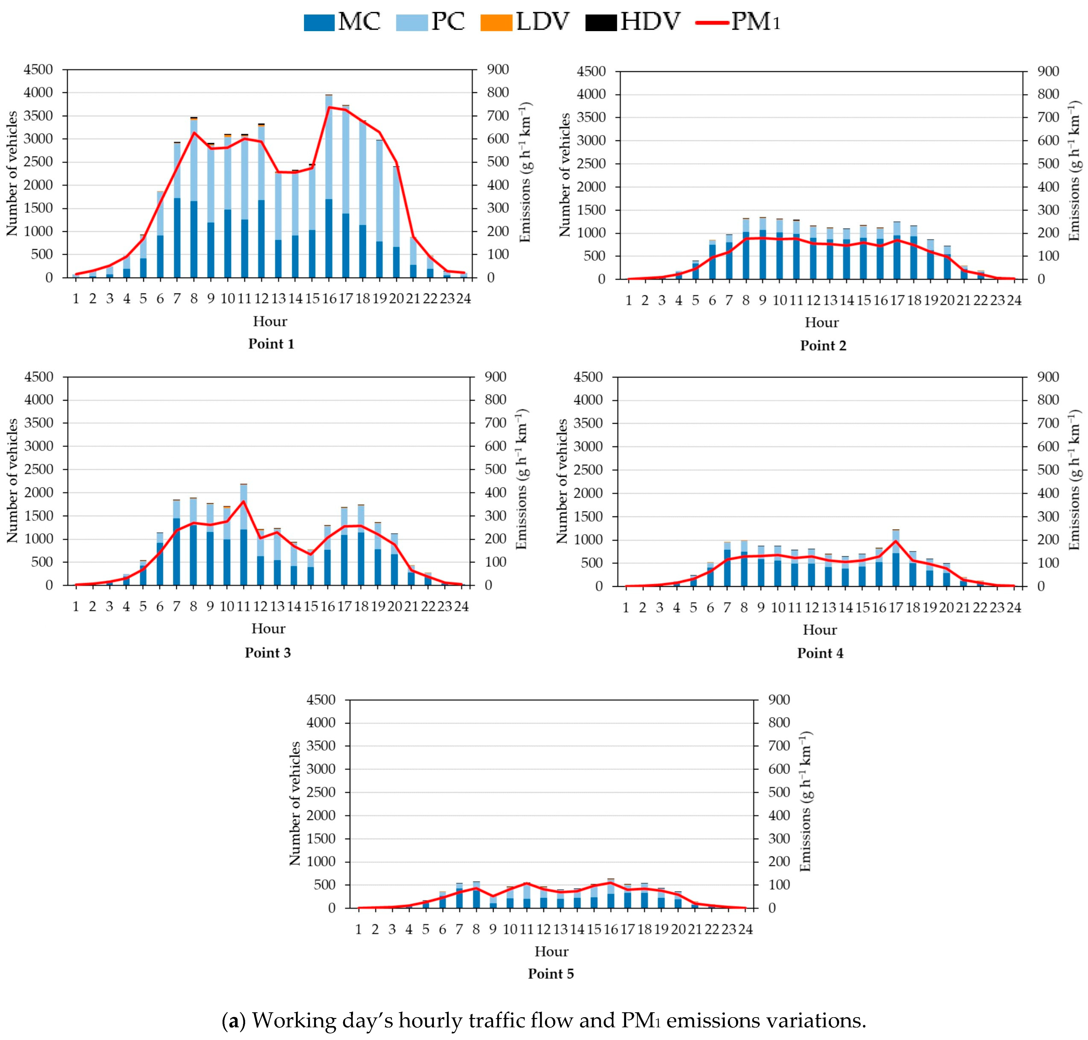
3.1.3. Temporal Variations in Traffic Emissions

Changes in hourly traffic flows at the five traffic counting points throughout the working day and on the weekend, as well as their corresponding PM₁ emission rates per distance traveled (g h⁻¹ km⁻¹) are illustrated in Figure 3. As expected, PM₁ emission rates per distance traveled varied in accordance with traffic activity. Times with less traffic resulted in emission rates notably lower than during peak hours because vehicles were more polluting in congested traffic, due to frequent low speed and idling [47,48]. The highest number of vehicles was recorded at point 1, with the fewest recorded at point 5. This is because point 1 was located at the main inbound and outbound route and had a fresh market each morning, while point 5 was linked to the low-density residential zone in the old town.

On working days (Figure 3a), more traffic was observed in the morning (07:00–11:00) and evening (16:00–18:00), as people went shopping at the morning market and traveled to work, then returned home in the evening. On the weekend, more traffic was observed at midday, lasting until nighttime (Figure 3b). Both residents and tourists spent their time outdoors during these periods, with many people engaged in sightseeing, eating, and shopping in the study area. If point 1 is taken to represent the traffic conditions in the study area, the variations on workdays and at weekends are comparable to those in Nakhon Pathom municipality, a city located in an adjacent province [49], and in Bangkok, Thailand’s capital [50], suggesting homogeneous traveling behaviors in Bangkok and its surrounding cities.

In addition, we used a multiple-linear regression model in Microsoft Excel to examine the contribution of the various categories of vehicles on PM₁ emissions. The least squares method was used to fit a line through the data. The dependent variable was PM₁ emissions per kilometer. The independent variables comprised the hourly numbers of MCs, PCs, LDVs, and HDVs combined for both working days and weekends at all observation points. The results can be seen in Equation (6).

$${\mathrm{PM}}_1=0.096 \mathrm{MC}+0.252 \mathrm{PC}+0.136 \mathrm{LDV}+0.716 \mathrm{HDV}$$

(6)

(n = 240, p-value < 0.01).

In Equation (6), HDVs had the highest coefficient values (0.719), followed by PCs (0.252), LDVs (0.136), and MCs (0.096). Each coefficient is interpreted as the estimated change in PM₁ corresponding to a one-unit change in a vehicle type, when all others are held constant. In other words, in our study, HDVs had the greatest influence on PM₁ emissions, while MCs had the least. This suggests that consideration should be given to banning HDVs from accessing the old town, although it was the least proportion found in the fleet.

3.2. Evaluation of R-LINE

Figure 4 shows a comparison between PM₁ concentrations yielded by R-LINE and the values obtained from the five measurement sites, averaged over monitoring hours (Figure 4a) and locations (Figure 4b). The simulated PM₁ showed greater deviations on a temporal basis than on a spatial basis. The greatest difference between the observed values (10.3 ± 1.3 µg m⁻³) and the simulated values (8.6 ± 0.5 µg m⁻³) occurred during rush hour at 08:00. Spatially, the simulated PM₁ values showed good agreement with the observed values (Figure 4b). R-LINE was also able to capture the highest PM₁ concentration, as observed at point 2.

For the statistical analyses, the results were also plotted as single hours (SH) and the average hourly value over the measurement period of 7 h (AH), as shown in Figure 5a,b, respectively. The NMSE values of SH and AH were 0.01 and 0.06, respectively, and the FB values of SH and AH were −0.01 and 0.21, respectively. These model performance evaluation indicators were all close to the ideal values (NMSE and FB = 0.0) [51]. The results were comparable to previously reported PM levels due to road traffic activities, simulated using a line source dispersion model, CALINE 4 (NMSE = 0.08 and FB = −0.01) [52], and a Lagrangian particle model, (GRAL) (NMSE = 0.04 and FB = 0.13) [53]. The simulation performance in our study is better than the performance reported in previous work using the WinOSPM, ADMS-Urban, and AEOLIUS models (in which NMSE ranged from 0.11 to 0.23 and FB ranged from −0.08 to 0.26) [54].

The scatter plots for both SH and AH were within the factor of 2 (FAC2) boundary. However, the AH plot (Figure 5b) was closer to a 1:1 line than that of SH (Figure 5a). The linear regression equations indicated that R-LINE’s predictions tended to be underestimates, especially in the case of SH. These underestimates may be due to the absence of a chemical transformation function in the current version of R-LINE [33,55], despite the fact that atmospheric chemical reactions play a vital role in forming secondary PM in the air [21]. The AH results from the simulations ranged from 8.2 to 10.1 µg m⁻³, which were close to the observations ranging from 7.8 to 9.7 µg m⁻³. Additionally, the R value of AH (0.89) was higher than that of SH (0.51), implying that AH was more suitable to be specified as the temporal basis for the R-LINE simulation.

It should be noted that we applied R-LINE on a daily basis, not on specific periods of time, such as AH. Due to the COVID-19 pandemic, however, we were unable to conduct monitoring for a longer period, which was a limitation of this study. Nevertheless, based on the model evaluation results of our work, as well as the results of previous studies (e.g., [33]), we believe that R-LINE was appropriate for our case study.

To examine the impact of meteorological conditions on PM₁ concentrations, the daily PM₁ values simulated over the year were compared with wind speed (WS) and atmospheric ventilation rates (VRATE), as shown in Figure 6 and Figure 7, respectively. The model results were categorized into two groups according to the wind speed conditions, i.e., low (WS ≤ 0.6 m s⁻¹) and high (WS > 0.6 m s⁻¹) wind-speed conditions. The low wind-speed classification was defined based on Ling and colleagues’ 2020 study [53], in which they carried out simulations of road-traffic PM in an Asian micro-scale urban environment, similar to our study.

As seen in Figure 6a, PM₁ concentrations increased during the low wind-speed regime and considerably declined when the wind speed was higher (Figure 6b). Low wind-speed conditions restricted the transport of air pollution, inducing the accumulation of air pollutants, especially at the extremely low wind-speed of less than 0.6 m s⁻¹ present in the study area. As expected, the PM₁ concentration was inversely correlated with VRATE; this was even more pronounced at higher wind speeds (Figure 7). VRATE is principally obtained by multiplying the wind speed by the height of the planetary boundary layer (PBL). Hence, a combination of high wind-speed and high PBL promotes good ventilation, resulting in better dispersion conditions and allowing PM₁ to be diluted [56,57]. The results of the correlations of PM₁ and the dynamic atmospheric parameters imply that the R-LINE model yielded reasonable results. However, the low statistical correlation suggested by the low Pearson correlation coefficients (the r values are provided in Figure 6 and Figure 7) implies that there are additional factors influencing the PM₁ concentration in the air. Thus, further research is necessary to explore air pollution dispersion, particularly under low wind-speed conditions.

3.3. Comparisons with Similar Studies

A comparison of PM₁ concentrations at our site and previously reported results is presented in

Table 3. PM₁ concentrations observed in the current study and in other studies.

Location	Source	PM1 (µg m−3) *	PM1/PM2.5 Ratio	Monitoring Period	Temporal Basis
Thailand (Ratchaburi old town/roadside)	This study	8.7 ± 0.8 a (7.8–9.7)	0.69	18 May 2022 (08:00–15:00, 7 h in total)	7 h average
		8.8 ± 0.7 b (8.2–10.1)	NA
Italy (Venice)	[21]	34 ± 24 a (winter) 6.4 ± 2.2 a (summer)	NA	December 2013–February 2014 (winter) May–July 2014 (summer)	Seasonal average
Algeria (Algiers/roadside)	[59]	5.93–46.08 a	0.55	1 January– 30 September 2015	Daily average
China (Hong Kong/roadside)	[60]	26.1 ± 0.7 a	NA	2 November– 13 December 2017	Daily average
China (Taichung, Taiwan)	[61]	11.05 ± 5.03 a (3.96–23.32)	0.73	15–22 April 14–23 May 2021	Daily average
China (73 cities across the entire mainland)	[62]	4.8–84.0 a	0.75–0.88	1 November 2013– 31 December 2014	Daily average
Europe (12 cities)	[63]	12.2 ± 9.3 a	NA	October 2015–April 2019	Average of different periods in each city
Austria (Graz)	[64]	20 ± 11.9 a (winter) 14.1 ± 6.5 a (summer)	0.78 (winter) 0.91 (summer)	October 2000–March 2001 (winter) April–September 2001 (summer)	Seasonal average
Turkey (Istanbul)	[65]	22.1 ± 6.4 a (7.6–30.2)	0.55	11 December 2009–9 April 2010	Daily average
India (Varanasi)	[66]	89.9 ± 44.4 a	0.84	April 2019–March 2020	Over the monitoring period

* Average value (single number); average value ± standard deviation; minimum value–maximum value; ^a monitoring results; ^b modeling results; NA, not available.

. The differences in PM₁ levels in a specific area depend on various factors, including emission sources; meteorological conditions; topography (e.g., complex or flat terrain) and land use (e.g., urban, suburban, rural); receptors (distances and heights in relation to the emission sources); and the timeframe under consideration (e.g., daily, seasonal, annual). Changes in behavior due to the COVID-19 pandemic could also have led to a decrease in road traffic-related particles [58] in our study area.

The ratios of PM₁ to PM_2.5 from our observations compared with other studies are also presented in Table 3. Our ratio (0.69) was lower than those obtained in studies from cities in China (0.75–0.88); Graz, Austria (0.78–0.91); and Varanasi, India (0.84); however, it was higher than those recorded in Istanbul, Turkey (0.55) and Algiers, Algeria (0.55), while it was comparable to that in Taichung, in Taiwan (0.73). High PM₁/PM_2.5 ratios imply that fine PM mainly comprises submicronic particles (PM₁) and has a greater health impact [59]. High PM₁/PM_2.5 ratios are often observed on days with high levels of pollution; high ratios are also more likely in urban areas than in rural areas, and in winter rather than summer. It also indicates the role of combustion processes and secondary particle formation [62]. As we conducted measurements at the roadside, the PM₁/PM_2.5 ratio implied that PM₁ mainly originated from internal combustion vehicles rather than the formation of secondary particles. This emphasized the importance of controlling these vehicles.

3.4. Changes of Vehicles in Our Case Studies’ Road Network

Observed hourly traffic volumes, both during the working day and on the weekend, on different road types (33 road segments in total) are averaged into daily mean values representing current traffic flows of the base case (BC), as presented in Figure 8. The switching of traffic activities from the cultural tourism road to the main road for S1 and S2 is also included. In BC, there were 44,903 vehicles daily on the cultural tourism route, slightly more than those on the main road, which had 42,187 vehicles. In S1, vehicles were assumed to be banned from driving on the cultural tourism route. Therefore, they were combined with those from the main road, resulting in an increased daily number of vehicles to 87,065. Traffic congestion, as well as high emissions of PM₁ due to road traffic, can be expected on the main road. In S2, the number of vehicles on the main road was assumed to decrease due to the mitigation measures, discussed later. Note that traffic activities on both the road connected to the highway and the secondary road were assumed to remain the same in all cases. In addition, note that the traffic activities in Figure 8 were previously allocated to the road segments, then multiplied by the corresponding PM₁ vehicle emission factors and incorporated in the R-LINE model to simulate changes in PM₁ concentration. The results are described later, in Section 3.5.

3.5. Spatial Distribution of PM₁ in the Case Studies

The simulations of PM₁ in BC, S1, and S2 are illustrated in Figure 9. Overall, they were consistent with the results of previous studies [34,67], showing high levels of traffic-induced fine PM pollution at roadsides, which rapidly decrease with increasing distance from roads. The fine PM contributed by road traffic can be heavily influenced by curbside traffic. A previous study involving a micro-scale PM simulation in an Asian community found that curbside traffic can contribute up to 40% of fine PM during rush hour [53]. The greatest PM₁ concentration was observed for the road connecting to the highway (the blue line in Figure 9). This was due to the large numbers of vehicles driven by residents and visitors, as seen in Figure 9 at point 1. Note that we added a PM₁ background concentration of 9.23 µg m⁻³, derived from the methodology mentioned earlier, to the model results.

In the short term, based on all of our case studies (BC, S1, and S2), policymakers can utilize the results to initiate ad hoc practical mitigation measures. For instance, high PM₁ concentrations regularly appeared on the western side (the red-colored band in Figure 9). Traffic management, e.g., switching traffic lanes to enhance traffic flows on connected-to-highway roads during traffic rush hours (seen in Figure 3) is recommended. Furthermore, pedestrians should be advised to minimize their outdoor activities to prevent exposure to PM near roadsides. Providing an air pollution monitoring system with a digital display screen showing the current air quality situation in this high pollution zone is recommended.

Interestingly, the PM₁ concentration along the river section was lower compared with the PM₁ concentrations in other parts of the study area. One reason for this is that it was away from the road-traffic emission sources. Another reason is that it supports the city’s aeration. This agrees with a recent study [68], in which black carbon was measured along bicycle routes in Wrocław, Poland. The study’s authors found that black carbon levels near to the river were noticeably lower than the levels near other routes in their study area. Rivers and embankments provide open spaces that promote better ventilation, which can dilute air pollution. Therefore, urban developers should incorporate open spaces. This will not only help in dispersing high concentrations of air pollution but also provide recreation areas for the public, including local citizens and visitors, and potentially further promoting tourism activities such as those in Ratchaburi’s old town.

The changes in PM₁ air contaminants in S1 and S2, compared to the reference BC, can be described as follows. For S1, all vehicles on the cultural tourism route (the yellow line in Figure 9) were made to drive on the main road (the green line in Figure 9); subsequently, there was an accumulation of vehicles and their emissions on the main road. Thus, elevated PM₁ levels were detected near the main road, while lower levels were detected near the cultural tourism route compared to BC.

For S1, vehicles were banned from the cultural tourism route, and visitors used another route, as closely as possible to the walking route. Therefore, it was not possible to avoid an accumulation of traffic and vastly increased levels of PM₁ on the main road. This would result in potentially adverse health outcomes for both the population living close to this road [69] and those traveling along footpaths [70]. In addition, this may cause the negative outcome of tourists ceasing to visit the cultural tourism route [12,71], which, in turn, affects the long-term success of car-free cultural tourism routes.

For the S2 scenario, it was assumed that none of the vehicles used to drive through the cultural tourism route would enter the study area. The overall number of vehicles and their PM₁ emissions were therefore reduced. Hence, clear decreases were seen in simulated PM₁ concentrations, both on the cultural tourism route and the main road. The changes in PM₁ concentrations at the five observation points are compared among the BC, S1, and S2 scenarios, as shown in Figure 10.

The S2 scenario was shown to be more suitable for the cultural tourism route than the S1 scenario. Mitigating road traffic was crucial to supporting the walkability of the cultural tourism route and achieving better air quality. However, S2 was more challenging in terms of traffic planning than S1. The S2 simulation suggested further traffic reduction measures would be needed, such as providing sufficient parking sites outside the focal area of the old town and appropriate vehicles, possibly electric buses, to shuttle visitors to the destination. Fortuitously, a new double-track railroad near the walkable cultural tourism route is almost complete, providing an ideal opportunity to minimize the number of personal vehicles in the area and promote the use of mass transit. Feasibility studies of such issues were beyond the scope of our work; however, we recommend conducting future studies to investigate this issue.

The practical implications of the environmental and economic aspects of implementing a walkable cultural tourism route in Ratchaburi’s old town are beyond the scope of our study and findings; however, it is crucial that they are discussed. From an environmental perspective, it is not only air pollution but also thermal comfort that can greatly influence pedestrians’ decision to walk [16]. Well-ventilated and shaded walkways along a pedestrian street can improve connectivity and comfort for tourists. Ensuring good sanitation and good practice in waste management (reduce, reuse, and recycle) are also recommended. From an economic perspective, tourism activities can provide income for local people. Increasing cultural tourism by using the Bio-Circular-Green Economic Model (BCG), introduced by the Thai research community and promoted by the Thai government as a new economic model [72], is feasible. For instance, the community could continue creating unique products with a history that reflects the local culture of Ratchaburi. Their production should also take into account the environment and sustainability, e.g., using local renewable biological resources and bio-based materials, with minimal pollution during production. Moreover, goods and services for tourism must be reasonably priced. Marketing via online applications is also encouraged to enhance product awareness at the same time as promoting tourism activities in the area. Finally, the income generated from tourism should be reinvested to support conservation programs for both tangible and intangible cultural resources in the old town. Multilateral collaboration among stakeholders, including relevant government organizations, local communities, nongovernmental organizations, and local enterprises, will be crucial for the creation and operation of the proposed plans. This aspect should also be considered in future studies.

Our study yielded several benefits. First, we evaluated the R-LINE model to ensure the trustworthiness of the simulation results, applying the model with high spatial resolution and refined traffic activity observations. Second, we investigated PM₁, a more useful tracker of traffic-induced air pollution than larger PM. Third, we demonstrated the possibility of determining the contribution of road vehicles to the reduced urban air quality, essential as PM₁ is now of great concern worldwide. Finally, this work supports the development of cultural tourism to help the environment, which is a key element if sustainable development of cultural tourism is to be achieved in urban areas [3].

Our study also had some limitations. First, the R-LINE model is unable to consider the arrangement of buildings, which can potentially obstruct air flow and the dispersion of air pollutants. This impact can be considerable under low wind-speed conditions. Second, the measurements used to evaluate the model’s performance were conducted during just a single day, due to restrictions imposed during the COVID-19 pandemic. Additionally, the measurement devices were based on light scattering, which is an alternative method to the method used for the official measurements of fine PM. Lastly, our study did not consider PM₁ emissions from other local sources, such as wood stoves for local streetside cooking and smoke from open air incense and joss paper burning. These are related to traditional activities in Asian communities and may become potentially important sources of emissions if visitor numbers increase.

4. Conclusions

Varying traffic activities to create a car-free cultural tourism route could affect the occurrence of PM₁ emissions and contribute to reduced air pollution in Ratchaburi’s old town. We found a consistency between hourly variations in traffic activities and PM₁ vehicle emissions in the old town, both on the working day and on the weekend. Our evaluation of the R-LINE model indicated its performance was acceptable to simulate PM₁ levels in the study area. Our study suggested that remarkable changes in PM₁ concentrations could be achieved through alterations in road traffic mitigation measures: promoting the use of a new double-track railroad near the walkable cultural tourism route; providing parking sites outside the central area of the old town; and using well-organized shuttle vehicles to transport visitors from both services to the walking street. These types of changes should be considered in future studies. We suggest that decision-makers and relevant stakeholders establish traffic management plans to sustainably develop the cultural tourism route in Ratchaburi’s old town.

References

1. World Travel & Tourism Council (WTTC). Economic Impact Research. 2023. Available online: https://wttc.org/research/economic-impact (accessed on 7 December 2023).
2. Eslami, F.; Namdar, R. Social, Environmental and Economic Impact Assessment of COVID-19 on Rural Tourism. Front. Public Health 2022, 10, 883277. [Google Scholar] [CrossRef] [PubMed]
3. Istoc, E. Urban cultural tourism and sustainable development. Int. J. Responsible Tour. 2012, 1, 38–57. [Google Scholar]
4. World Tourism Organization (UNWTO). Cultural Tourism and COVID-19. 2020. Available online: https://www.unwto.org/cultural-tourism-covid-19 (accessed on 18 December 2023).
5. The Royal Thai Government Gazette. Regulation of the Prime Minister’s Office on the Conservation and Development of Rattanakosin Area and Old Towns 2021. 2021. Available online: https://dl.parliament.go.th/handle/20.500.13072/584997 (accessed on 18 December 2023). (In Thai).
6. Office of Natural Resources and Environmental Policy and Planning (ONEP). Environmental Quality Situation in 2022 (Infographic Edition). 2023. Available online: https://www.onep.go.th/book/info-soe2565/ (accessed on 26 July 2023).
7. Chaiyapotpanit, A.; Khaokhiew, C.; Thamrungraeng, R.; Chantaruphan, P.; Sinvuttaya, S.; Preamkulanan, P.; Tangcharatwong, K.; Jitpaisarnwattana, N.; Maneechote, M.; Rujirotvarangkul, C. Cultural capital for the development and conservation of ancient cities in western Thailand: A case study of the Ratchaburi and Phetchaburi provinces. Humanit. Arts Soc. Sci. Stud. 2023, 23, 528–538. [Google Scholar] [CrossRef]
8. Preyawanit, N. Ratchaburi old town: A preservation and development study. NAJUA Hist. Archit. Thai Archit. 2023, 20, 160–197. (In Thai) [Google Scholar]
9. Silpakorn University. The Conservation and Development of Ratchaburi Old Town Towards Creative and Livable City for Cultural-Based Economic Advancement and Sustainable Living; Silpakorn University Research, Innovation and Creativity (SURIC) Administration Office: Phetchaburi, Thailand, 2020. (In Thai) [Google Scholar]
10. Sunlu, U. Environmental impacts of tourism. In Local Resources and Global Trades: Environments and Agriculture in the Mediterranean Region; Camarda, D., Grassini, L., Eds.; CIHEAM: Bari, Italy, 2003; pp. 263–270. [Google Scholar]
11. Belsoy, J.; Korir, J.; Yego, J. Environmental Impacts of Tourism in Protected Areas. J. Environ. Earth Sci. 2012, 10, 64–73. [Google Scholar]
12. Eusébio, C.; Carneiro, M.J.; Madaleno, M.; Robaina, M.; Rodrigues, V.; Russo, M.; Relvas, H.; Gama, C.; Lopes, M.; Seixas, V.; et al. The impact of air quality on tourism: A systematic literature review. J. Tour. Futures 2020, 7, 111–130. [Google Scholar] [CrossRef]
13. Zhao, S.; Li, Q.; Kong, Y.; Chen, X. The coupling relationship between tourism economy and air quality in China: A province-level analysis. J. Environ. Econ. Manag. 2023, 11, 1111828. [Google Scholar] [CrossRef]
14. Oliveira, M.L.; Neckel, A.; Pinto, D.; Maculan, L.S.; Dotto, G.L.; Silva, L.F. The impact of air pollutants on the degradation of two historic buildings in Bordeaux, France. Urban Clim. 2021, 39, 100927. [Google Scholar] [CrossRef]
15. Daengprathum, N.; Onchang, R.; Nakhapakorn, K.; Robert, O.; Tipayarom, A.; Sturm, P.J. Estimation of Effects of Air Pollution on the Corrosion of Historical Buildings in Bangkok. Environ. Nat. Resour. J. 2022, 20, 505–545. [Google Scholar] [CrossRef]
16. Baobeid, A.; Koç, M.; Al-Ghamdi, S.G. Walkability and its relationships with health, sustainability, and livability: Elements of physical environment and evaluation frameworks. Front. Built Environ. 2021, 7, 721218. [Google Scholar] [CrossRef]
17. Jeong, I.; Choi, M.; Kwak, J.; Ku, D.; Lee, S. A comprehensive walkability evaluation system for promoting environmental benefits. Sci. Rep. 2023, 13, 16183. [Google Scholar] [CrossRef] [PubMed]
18. Hu, Y.; Wu, M.; Li, Y.; Liu, X. Influence of PM1 exposure on total and cause-specific respiratory diseases: A systematic review and meta-analysis. Environ. Sci. Pollut. Res. 2022, 29, 15117–15126. [Google Scholar] [CrossRef] [PubMed]
19. Zhang, Y.; Ding, Z.; Xiang, Q.; Wang, W.; Huang, L.; Mao, F. Short-term effects of ambient PM1 and PM2.5 air pollution on hospital admission for respiratory diseases: Case-crossover evidence from Shenzhen, China. Int. J. Hyg. Environ. Health 2020, 224, 113418. [Google Scholar] [CrossRef] [PubMed]
20. Pope, C.A.; Dockery, D.W. Health effects of fine particulate air pollution: Lines that connect. J. Air Waste Manag. Assoc. 2006, 56, 709–742. [Google Scholar] [CrossRef]
21. Squizzato, S.; Masiol, M.; Agostini, C.; Visin, F.; Formenton, G.; Harrison, R.M.; Rampazzo, G. Factors, origin and sources affecting PM1 concentrations and composition at an urban background site. Atmos. Res. 2016, 180, 262–273. [Google Scholar] [CrossRef]
22. Giechaskiel, B.; Melas, A.; Martini, G.; Dilara, P.; Ntziachristos, L. Revisiting Total Particle Number Measurements for Vehicle Exhaust Regulations. Atmosphere 2022, 13, 155. [Google Scholar] [CrossRef]
23. Bond, T.C.; Doherty, S.J.; Fahey, D.W.; Forster, P.M.; Berntsen, T.; DeAngelo, B.J.; Flanner, M.G.; Ghan, S.; Kärcher, B.; Koch, D.; et al. Bounding the role of black carbon in the climate system: A scientific assessment. J. Geophys. Res. Atmos. 2013, 118, 5380–5552. [Google Scholar] [CrossRef]
24. Grivas, G.; Stavroulas, I.; Liakakou, E.; Kaskaoutis, D.G.; Bougiatioti, A.; Paraskevopoulou, D.; Gerasopoulos, E.; Mihalopoulos, N. Measuring the Spatial Variability of Black Carbon in Athens during Wintertime. Air Qual. Atmos. Health 2019, 12, 1405–1417. [Google Scholar] [CrossRef]
25. International Agency for Research on Cancer (IARC). Diesel and Gasoline Engine Exhausts and Some Nitroarenes. IARC Monographs on the Evaluation of Carcinogenic Risks to Humans; International Agency for Research on Cancer: Lyon, France, 2014; Volume 105, ISBN 13-978-9283213284. [Google Scholar]
26. Fanick, E.R.; Whitney, A.K.; Bailey, K.B. Particulate Characterization Using Five Fuels. J. Fuels Lubr. 1996, 105, 647–655. [Google Scholar]
27. Ristovski, Z.D.; Morawska, L.; Hitchins, J.; Thomas, S.; Greenaway, C.; Gilbert, D. Particle emissions from compressed natural gas engines. J. Aerosol Sci. 2000, 31, 403–413. [Google Scholar] [CrossRef]
28. Ristovski, Z.D.; Jayaratne, E.R.; Morawska, L.; Ayoko, G.A.; Lim, M. Particle and carbon dioxide emissions from passenger vehicles operating on unleaded petrol and LPG fuel. Sci. Total Environ. 2005, 345, 93–98. [Google Scholar] [CrossRef]
29. Kwak, J.H.; Kim, H.S.; Lee, J.H.; Lee, S.H. On-road chasing measurement of exhaust particle emissions from diesel, CNG, LPG, and DME-fueled vehicles using a mobile emission laboratory. Int. J. Automot. Technol. 2014, 15, 543–551. [Google Scholar] [CrossRef]
30. Karjalainen, P.; Pirjola, L.; Heikkilä, J.; Lähde, T.; Tzamkiozis, T.; Ntziachristos, L.; Keskinen, J.; Rönkkö, T. Exhaust particles of modern gasoline vehicles: A laboratory and an on-road study. Atmos. Environ. 2014, 97, 262–270. [Google Scholar] [CrossRef]
31. Stavroulas, I.; Grivas, G.; Liakakou, E.; Kalkavouras, P.; Bougiatioti, A.; Kaskaoutis, D.G.; Lianou, M.; Papoutsidaki, K.; Tsagkaraki, M.; Zarmpas, P.; et al. Online Chemical Characterization and Sources of Submicron Aerosol in the Major Mediterranean Port City of Piraeus, Greece. Atmosphere 2021, 12, 1686. [Google Scholar] [CrossRef]
32. Biró, N.; Kiss, P. Euro VI-d Compliant Diesel Engine’s Sub-23 nm Particle Emission. Sensors 2023, 23, 590. [Google Scholar] [CrossRef] [PubMed]
33. Snyder, M.G.; Venkatram, A.; Heist, D.K.; Perry, S.G.; Petersen, W.B.; Isakov, V. RLINE: A line source dispersion model for near-surface releases. Atmos. Environ. 2013, 77, 748–756. [Google Scholar] [CrossRef]
34. Park, Y.M. Assessing personal exposure to traffic-related air pollution using individual travel-activity diary data and an on-road source air dispersion model. Health Place 2020, 63, 102352. [Google Scholar] [CrossRef] [PubMed]
35. Rodriguez-Rey, D.; Guevara, M.; Linares, M.P.; Casanovas, J.; Armengol, J.M.; Benavides, J.; Soret, A.; Jorba, O.; Tena, C.; García-Pando, C.P. To What Extent the Traffic Restriction Policies Applied in Barcelona City Can Improve Its Air Quality? Sci. Total Environ. 2022, 807, 150743. [Google Scholar] [CrossRef]
36. Ma, T.; Li, C.; Luo, J.; Frederickson, C.; Tang, T.; Durbin, T.D.; Johnson, K.C.; Karavalakis, G. In-Use NOx and Black Carbon Emissions from Heavy-Duty Freight Diesel Vehicles and near-Zero Emissions Natural Gas Vehicles in California’s San Joaquin Air Basin. Sci. Total Environ. 2024, 907, 168188. [Google Scholar] [CrossRef]
37. Choi, K.; Chong, K. Modified Inverse Distance Weighting Interpolation for Particulate Matter Estimation and Mapping. Atmosphere 2022, 13, 846. [Google Scholar] [CrossRef]
38. Kupiainen, K.; Klimont, Z. Primary Emissions of Submicron and Carbonaceous Particles in Europe and the Potential for their Control; International Institute for Applied Systems Analysis: Luxembourg, 2004. [Google Scholar]
39. European Environment Agency (EEA). EMEP/EEA Air Pollutant Emission Inventory Guidebook 2019 Technical Guidance to Prepare National Emission Inventories; European Environment Agency: Kongens Nytorv, Denmark, 2019; Volume 13, ISSN 1977-8449. [Google Scholar]
40. Department of Land Transport (DLT). Transport Statistic Report 2022. 2023. Available online: https://web.dlt.go.th/statistics/ (accessed on 24 December 2023).
41. Thai Meteorological Department (TMD). Meteorological Measurement and Statistics Service. 2019. Available online: https://www.tmd.go.th/service/tmdData (accessed on 9 December 2021).
42. Meteoblue AG. Historical Weather Data 2019. 2021. Available online: https://www.meteoblue.com/weather/archive/export (accessed on 12 December 2021).
43. Pace, T.G. Chapter 8—Receptor Modeling in the Context of Ambient Air Quality Standard for Particulate Matter. Data Handl. Sci. Technol. 1991, 7, 255–297. [Google Scholar] [CrossRef]
44. Bigi, A.; Ghermandi, G. Particle Number Size Distribution and Weight Concentration of Background Urban Aerosol in a Po Valley Site. Water Air Soil Pollut. 2011, 220, 265–278. [Google Scholar] [CrossRef]
45. Department of Land Transport (DLT). Transport Statistic Report Fiscal Year 2019–2023. 2023. Available online: https://web.dlt.go.th/statistics/plugins/UploadiFive/uploads/6f6897ce35cd1d6a488eab4c29a548a0b5d0973421176078322eff0d7d61b5a5.pdf (accessed on 24 December 2023).
46. Oliveira, L.K.D.; Cordeiro, C.H.D.O.L.; Oliveira, I.K.D.; Andrade, M. Exploring the relationship between socioeconomic and delivery factors, traffic violations, and crashes involving motorcycle couriers. Case Stud. Transp. Policy 2024, 15, 101111. [Google Scholar] [CrossRef]
47. Zhang, Y.; Deng, W.; Hu, Q.; Wu, Z.; Yang, W.; Zhang, H.; Wang, Z.; Fang, Z.; Zhu, M.; Li, S.; et al. Comparison between idling and cruising gasoline vehicles in primary emissions and secondary organic aerosol formation during photochemical ageing. Sci. Total Environ. 2020, 722, 137934. [Google Scholar] [CrossRef] [PubMed]
48. Wang, P.; Zhang, R.; Sun, S.; Gao, M.; Zheng, B.; Zhang, D.; Zhang, Y.; Carmichael, G.R.; Zhang, H. Aggravated air pollution and health burden due to traffic congestion in urban China. Atmos. Chem. Phys. 2023, 23, 2983–2996. [Google Scholar] [CrossRef]
49. Onchang, R.; Noisopa, K.; Pawarmart, I. Changes of Air Pollution and Climate Forcing Emissions due to Fuel Switching to Gasohol in Motorcycle Fleet in an Urban Area of Thailand. EnvironmentAsia 2017, 10, 94–104. [Google Scholar] [CrossRef]
50. Naiudomthum, S.; Winijkul, E.; Sirisubtawee, S. Near Real-Time Spatial and Temporal Distribution of Traffic Emissions in Bangkok Using Google Maps Application Program Interface. Atmosphere 2022, 13, 94–104. [Google Scholar] [CrossRef]
51. Chang, J.C.; Hanna, S.R. Air quality model performance evaluation. Meteorol. Atmos. Phys. 2004, 87, 167–196. [Google Scholar] [CrossRef]
52. Yu, S.; Chang, C.T.; Ma, C.M. Simulation and Measurement of Air Quality in the Traffic Congestion Area. Sustain. Environ. Res. 2021, 31, 26. [Google Scholar] [CrossRef]
53. Ling, H.; Candice Lung, S.-C.; Uhrner, U. Micro-Scale Particle Simulation and Traffic-Related Particle Exposure Assessment in an Asian Residential Community. Environ. Pollut. 2020, 266, 115046. [Google Scholar] [CrossRef]
54. Vardoulakis, S.; Valiantis, M.; Milner, J.; ApSimon, H. Operational Air Pollution Modelling in the UK-Street Canyon Applications and Challenges. Atmos. Environ. 2007, 41, 4622–4637. [Google Scholar] [CrossRef]
55. Batterman, S.A.; Berrocal, V.J.; Milando, C.; Gilani, O.; Arunachalam, S.; Zhang, K.M. Enhancing models and measurements of traffic-related air pollutants for health studies using dispersion modeling and Bayesian data fusion. Health Eff. Inst. 2020, 202, 7313251. [Google Scholar]
56. Srimuruganandam, B.; Shiva Nagendra, S.M. Analysis and Interpretation of Particulate Matter—PM10, PM2.5 and PM1 Emissions from the Heterogeneous Traffic near an Urban Roadway. Atmos. Pollut. Res. 2010, 1, 184–194. [Google Scholar] [CrossRef]
57. Shelton, S.; Liyanage, G.; Jayasekara, S.; Pushpawela, B.; Rathnayake, U.; Jayasundara, A.; Jayasooriya, L.D. Seasonal Variability of Air Pollutants and Their Relationships to Meteorological Parameters in an Urban Environment. Adv. Meteorol. 2022, 2022, 5628911. [Google Scholar] [CrossRef]
58. Polednik, B. COVID-19 lockdown and particle exposure of road users. J. Transp. Health 2021, 22, 101233. [Google Scholar] [CrossRef]
59. Talbi, A.; Kerchich, Y.; Kerbachi, R.; Boughedaoui, M. Assessment of annual air pollution levels with PM1, PM2.5, PM10 and associated heavy metals in Algiers, Algeria. Environ. Pollut. 2018, 232, 252–263. [Google Scholar] [CrossRef] [PubMed]
60. Yao, D.; Lyu, X.; Lu, H.; Zeng, L.; Liu, T.; Chan, C.K.; Guo, H. Characteristics, sources and evolution processes of atmospheric organic aerosols at a roadside site in Hong Kong. Atmos. Environ. 2021, 252, 118298. [Google Scholar] [CrossRef]
61. Fang, G.C.; Peng, Y.P.; Zhuang, Y.J.; Huang, L.C. Monitoring ambient air particulates, VOC and CO2 pollutants concentrations, particulates numbers by AQ Guard Ambient sampler. Environ. Forensics 2022, 24, 218–225. [Google Scholar] [CrossRef]
62. Chen, G.; Morawska, L.; Zhang, W.; Li, S.; Cao, W.; Ren, H.; Wang, B.; Wang, H.; Knibbs, L.D.; Williams, G.; et al. Spatiotemporal variation of PM1 pollution in China. Atmos. Environ. 2018, 178, 198–205. [Google Scholar] [CrossRef]
63. Chen, G.; Canonaco, F.; Tobler, A.; Aas, W.; Alastuey, A.; Allan, J.; Atabakhsh, S.; Aurela, M.; Baltensperger, U.; Bougiatioti, A.; et al. European aerosol phenomenology—8: Harmonised source apportionment of organic aerosol using 22 Year-long ACSM/AMS datasets. Environ. Int. 2022, 166, 107325. [Google Scholar] [CrossRef]
64. Gomišček, B.; Hauck, H.; Stopper, S.; Preining, O. Spatial and Temporal Variations of PM1, PM2.5, PM10 and Particle Number Concentration during the AUPHEP—Project. Atmos. Environ. 2004, 38, 3917–3934. [Google Scholar] [CrossRef]
65. Onat, B.; Sahin, U.A.; Akyuz, T. Elemental characterization of PM2.5 and PM1 in dense traffic area in Istanbul, Turkey. Atmos. Pollut. Res. 2013, 4, 101–105. [Google Scholar] [CrossRef]
66. Chauhan, P.K.; Kumar, A.; Pratap, V.; Singh, A.K. Seasonal Characteristics of PM1, PM2.5, and PM10 over Varanasi during 2019–2020. Front. Sustain. Cities 2022, 4, 101–105. [Google Scholar] [CrossRef]
67. Askariyeh, M.H.; Zietsman, J.; Autenrieth, R. Traffic contribution to PM2.5 increment in the near-road environment. Atmos. Environ. 2020, 224, 117113. [Google Scholar] [CrossRef]
68. Kamińska, J.A.; Turek, T.; Van Poppel, M.; Peters, J.; Hofman, J.; Kazak, J.K. Whether Cycling around the City Is in Fact Healthy in the Light of Air Quality-Results of Black Carbon. J. Environ. Manag. 2023, 337, 117694. [Google Scholar] [CrossRef]
69. Huang, S.; Lawrence, J.; Kang, C.M.; Li, J.; Martins, M.; Vokonas, P.; Gold, D.R.; Schwartz, J.; Coull, B.A.; Koutrakis, P. Road proximity influences indoor exposures to ambient fine particle mass and components. Environ. Pollut. 2018, 243, 978–987. [Google Scholar] [CrossRef]
70. Zhu, C.; Fu, Z.; Liu, L.; Shi, X.; Li, Y. Health risk assessment of PM2.5 on walking trips. Sci. Rep. 2021, 11, 19249. [Google Scholar] [CrossRef]
71. Srinamphon, P.; Chernbumroong, S.; Tippayawong, K.Y. The effect of small particulate matter on tourism and related SMEs in Chiang Mai, Thailand. Sustainability 2022, 14, 8147. [Google Scholar] [CrossRef]
72. Asia-Pacific Economic Cooperation. Understanding the Bio-Circular-Green (BCG) Economy Model. 2022. Available online: https://www.apec.org/publications/2022/08/understanding-the-bio-circular-green-(bcg)-economy-model (accessed on 25 February 2023).
Figure 1. Location of the study area in Ratchaburi’s old town, western Thailand.
Atmosphere 15 00377 g001
Figure 2. Daily numbers of vehicles recorded in the monitoring locations.
Atmosphere 15 00377 g002
Figure 3. Variations in hourly traffic flow and PM1 emissions during working days (a) and on the weekend (b).
Atmosphere 15 00377 g003aAtmosphere 15 00377 g003b
Figure 4. Observed vs. simulated PM1 and observed PM2.5 during the monitoring period from 08:00 to 14:00 (averaged over the five roadside locations) (a) and at the five roadside locations (averaged over the monitoring period) (b).
Atmosphere 15 00377 g004
Figure 5. Observed vs. simulated hourly PM1 (SH) (a) and averaged values over the monitoring period (7 h) (AH) (b) at the five roadside locations. Note: dashed lines show the boundaries of 1:1 and a factor of 2; solid line, linear trendline; a background concentration of 5.5 µg m−3 was included in the model results.
Atmosphere 15 00377 g005
Figure 6. Variations of calculated PM1 at low wind-speed (WS ≤ 0.6 m s−1) (a) and higher wind-speed (WS > 0.6 m s−1) (b) at the fixed monitoring site (Point 3 in Figure 1); solid line, linear trendline; r, Pearson correlation coefficient.
Atmosphere 15 00377 g006
Figure 7. Variations in calculated PM1 at the atmospheric ventilation rate (VRATE), categorized into low wind-speed (WS ≤ 0.6 m s−1) (a) and higher wind-speed (WS > 0.6 m s−1) (b) conditions at the fixed monitoring site (around point 3 in Figure 1); solid line, linear trendline; r, Pearson correlation coefficient. The ventilation rates were estimated from the Global Forecast System (GFS), National Centers for Environmental Prediction (NCEP), USA, and provided by TMD.
Atmosphere 15 00377 g007
Figure 8. Changes in the mean traffic flows for the BC, S1, and S2 simulations at the different road types, with a total of 33 segments. (The locations of the roads in the study area are shown in Figure 1, with the colors of the bars in this figure being the same as the road line colors.)
Atmosphere 15 00377 g008
Figure 9. Daily PM1 concentrations attributable to on-road vehicle sources in BC, S1, and S2.
Atmosphere 15 00377 g009
Figure 10. Differences in simulated daily PM1 levels in the BC, S1, and S2 scenarios at the observation sites. (Figures with a minus sign indicate percentage reductions in PM1 compared to the BC values.)
Atmosphere 15 00377 g010