
Meteor Radar for Investigation of the MLT Region: A Review

1
ATRAD Pty Ltd., Adelaide, SA 5032, Australia
2
School of Physical Sciences, University of Adelaide, Adelaide, SA 5005, Australia
Atmosphere 2024, 15(4), 505; https://doi.org/10.3390/atmos15040505
Submission received: 20 February 2024
/
Revised: 10 April 2024
/
Accepted: 13 April 2024
/
Published: 20 April 2024
(This article belongs to the Special Issue Observations and Analysis of Upper Atmosphere)
Abstract
:This is an introductory review of modern meteor radar and its application to the measurement of the dynamical parameters of the Mesosphere Lower Thermosphere (MLT) Region within the altitude range of around 70 to 110 km, which is where most meteors are detected. We take a historical approach, following the development of meteor radar for studies of the MLT from the time of their development after the Second World War until the present. The application of the meteor radar technique is closely aligned with their ability to make contributions to Meteor Astronomy in that they can determine meteor radiants, and measure meteoroid velocities and orbits, and so these aspects are noted when required. Meteor radar capabilities now extend to measurements of temperature and density in the MLT region and show potential to be extended to ionospheric studies. New meteor radar networks are commencing operation, and this heralds a new area of investigation as the horizontal spatial variation of the upper-atmosphere wind over an extended area is becoming available for the first time.
1. Introduction
As the Earth moves around the Sun, it encounters small bodies in solar orbit. These consist mostly of debris from asteroids, some material ejected from comets, and interplanetary dust. Objects having sizes between 30 µm and 1 m are classed as ‘meteoroids’ [1,2]. Objects smaller than this are classed as interplanetary dust, and larger than this are classed as asteroids. These objects enter the atmosphere at speeds of between and (but meteoroids enter mostly between about and [3,4], and produce a meteor, a meteor being defined as the physical phenomena that result from the entry of the meteoroid). Phenomena may include the generation of heat, light, and ionization. Optical meteors result from the light produced by the meteoroid as it ablates in the atmosphere. ‘Fireballs’ are extremely bright optical meteors that result from meteoroids in the decimeter to meter size range. Meteoroids in the decimeter to half-centimeter size range typically produce those optical meteors that are detected with either video or still cameras [5]. Of course, there is also a dependence on the entry speed, and smaller, very fast meteoroids can produce bright trails.
Radio meteors, that is, meteors detected by the return of radio waves from the ionised meteor trail, are typically in the size range of 100 µm to 1 mm [6], but this does depend on the characteristics of the equipment being used. For the typical small meteor radars that are the focus of this review, the median initial diameter is in the range of about 500 to 700 µm [7], firmly in the meteoroid size range. Radio meteor detections have the advantage over optical detections of extending to much smaller initial particles, and the obvious advantage of being detected both day and night, and in poor seeing conditions.
1.1. Meteor Source Regions
Some meteoroids have a residual memory of their source body and give rise to meteor showers and appear to originate from a particular position in the sky known as its ‘radiant’. Showers occur with repetition periods associated with their source-body orbits, and many occur annually. Older material whose orbits have been randomised occur as sporadic background meteors. Sporadic meteors comprise the great majority of meteoroid material entering the atmosphere [8].
As a result of the Earth’s motion around the Sun and the distribution of the orbits of meteoroids about it, sporadic meteors appear to originate primarily from six diffuse structures about 15–20° wide, and detection rates vary with latitude, time of day, and season. The source regions are described in relation to the orbital motion of the Earth and the direction of the Sun from the Earth. The north and south apex sources lie about 15° above and below the direction of the orbital motion of the Earth. The helion and anti-helion sources are towards and away from the Sun as seen from the Earth, respectively. The north and south toroidal sources are located about 60° above and below the orbital motion of the Earth [3,9,10].
An example of the annual height and time variation of meteor detections for two meteor radars operating at two different frequencies at Davis Station (68.6° S, 77.9° E) in Antarctica is shown in Figure 1. Inspection of these plots indicates variations in the count rates, peak heights, and the widths of the distribution of the meteor detections in height through the year, with lower counts and overall peak heights in Austral winter and spring. In summer and autumn, the South Pole is tilted towards the sources located in the orbital apex and anti-helion directions and the counts are highest. The lowest count rate occurs in spring as the southern polar region is tilted away from the direction of the Earth’s direction of orbital motion and so is shielded from the dominant sources of sporadic meteors. The height distributions are also influenced by the background atmospheric conditions. For example, peak heights are lower in winter when the atmosphere is warmer and density lower and meteors can penetrate further into the atmosphere before starting to ionise. Note also that the 33.2 MHz peak height is higher than the 55 MHz radar peak height. Generally, the lower the frequency, the higher the peak of the distribution, as we discuss in the next section. These meteor radars utilise a broad beam directed vertically on transmission and five receive antennas arranged as an interferometer on reception. We describe this type of radar in more detail below.
1.2. Radar Detection of Meteors
Most meteors are now detected with radar, and so we now look at the formation of the meteor trail in a little more detail. Once in the atmosphere, collisions with atmospheric molecules convert meteoroid kinetic energy into heat (the gas mean free path is much much greater than the meteoroid radius). Evaporated material collides with atmospheric molecules () at meteoric speeds, and is rapidly slowed to thermal velocities, losing electrons to form a column of ionised material (plasma) behind the meteoroid which extends radially from the trail axis. Meteor trails are formed almost instantly behind an ablating meteoroid with an initial trail radius determined by the background atmospheric density. Most radar meteors are detected in the 120 to 70 km height region, but the detection heights depend particularly on the radar wavelength, with the peak of the meteor detection distribution being higher the lower the frequency. This is because if the trail radius exceeds about the radiation scattered from the near and far parts of the train destructively interferes, and the echo is strongly attenuated (see e.g., [13,14]). Furthermore, higher radar frequencies require higher trail plasma densities to produce scattering. At higher altitudes, the ambipolar diffusion is very high and the trail expansion is very rapid. This means that higher frequency radars may not see the early stages of the trail development when the plasma density is high enough to produce a return. This means that there is a radar detection ceiling above which typical meteor radars see no meteors because the radar frequencies required to get to heights above about 110 km are low, and subject to ionospheric effects, radio interference, and practical limitations on antenna size. The expected performance of a meteor radar can be investigated in detail because its response to meteors associated with a particular radiant for all positions of the radiant in elevation and azimuth can be calculated to give the “response function” of the radar system (see e.g., [15]).
McKinley [16] gives the meteor count rate N dependent on transmitted power PT, radar wavelength λ (essentially the reciprocal of the operating frequency), system gain G, and received power PR as follows:
For the observations shown in Figure 1, the 55 MHz meteor radar shares the same hardware, but uses a separate transmitting and receiving array to the Davis (M)ST VHF radar. It is interleaved with other experiments on the radar. This leads to low count rates. Inspection of Equation (1) indicates that meteor counts are proportional to , so operating a meteor radar at 55 MHz would result in fewer counts than for an equivalent 33.2 MHz radar. In the case of Figure 1, the 55 MHz radar operated at a peak power of about 17 kW, and the 33.2 MHz radar at a peak power of 7.5 kW. Complete descriptions of these radars are given in [12].
Radars detect meteors by transmitting radio waves which are then reflected and received back from this ionised column. To receive the return, the radio waves must be perpendicular to the trail. This is known as the ‘transverse’ condition as shown in Figure 2. In fully ‘underdense’ trails (, but see the discussion below), free electrons scatter radio waves coherently and independently and the return is referred to as being ‘specular’ (sometimes ‘classical’). The echo from the meteor trail corresponds to Fresnel scatter with the form of the diffraction pattern from a straight edge familiar from optics.
Following formation, underdense trails expand radially and the radar returned power in the form of the Fresnel diffraction pattern falls off exponentially with time. Figure 3 shows an example of a meteor trail echo. There are 1024 radar pulses in a second in this case. In this example, the Fresnel fringes are evident but not particularly clear. The time between the first maximum and the first minimum in the amplitude can be used to determine the meteoroid velocity in about 10% of returns [17]. Improved techniques using Fresnel transforms fitting for meteoroid speed have been developed that work for about 70% of meteor echoes [18,19,20].
The ionised meteor trail drifts with the background wind and can act as a target for a radar and so as a ‘tracer ‘of the background wind. This is the section of the trail echo after the time shown in Figure 2 and Figure 3, where the time rate of change in the phase gives the trail radial drift velocity. Note that the trail lifetimes in this case are much shorter than one second and this is typical for underdense trails used for wind determinations.
After formation, the ionised material diffuses outward. Assuming a Gaussian initial distribution, the diffusion-induced outward expansion of the trail causes the exponential decay of echo strength mentioned above (see Figure 3) with a particular time constant, τ given by:
where the ambipolar diffusion coefficient, , is determined by the ionic makeup and local atmosphere. The mean τ can be calculated over a suitable period as shown in Figure 4, (in this case 24 h), and so can be determined. We note that the bulk electron motion is constrained by quasi-neutrality, so that it is the ionic mobility that determines rate of diffusion.
For fully ‘overdense’ trails, the scattering is equivalent to that from a metallic cylinder. In this case, the radar returned power is almost unaffected by the trail expansion until the electron density has fallen enough for the trail to become underdense, at which time the returned power begins to fall off exponentially. Overdense trails are typically much longer lived than underdense trails and so can be significantly distorted by background winds. In this case, they are less suitable to simply determine the background wind. Ref. [22] used a full-wave scattering theory analysis to set the boundaries between overdense and underdense trails in terms of line densities as being for overdense trails, between as transition region, and below this as underdense trails. More recently, refs. [23,24] have quantitatively examined the theory described by [22] for different frequencies and polarizations. Their work showed a more complicated situation in which there is an altitude dependency resulting from the variation in radiative damping or collision frequencies with height. The transition from underdense to overdense trails might then depend on the radar frequency rather than the absolute line density and ref. [24] provides look up tables for six frequencies between 17.45 and 53.5 MHz.
The ionization around the incoming meteoroid can also be used as a target and so its radiant and speed through the atmosphere can be determined. Such echoes are known as ‘head’ echoes (sometimes ‘down-the-beam’ echoes (see e.g., [25]) when using narrow beam radars) as opposed to ‘trail’ echoes (see below). There is another class of echoes which are also sometimes known as ‘anomalous’ echoes, ‘non-classical’ echoes, and ‘non-specular’ echoes. For a further discussion of nomenclature see [26].
‘Non-classical’ echoes have been observed since the earliest radio observations of meteors [27]. Here, we will refer to them as ‘non-specular’ echoes but note that they have also been described as ‘range spread trail echoes’ or ‘RSTE’s: meaning that the radar meteor trail is spread in both range and time. An example showing a head echo and non-specular echo measured with the MIOS combined radio optical meteor and ionospheric irregularity observatory [28] and an ‘all-sky’ meteor radar at Ledong is shown in Figure 5. More recently, non-specular echoes have been further classified into Field-Aligned Irregularity (FAI) and Non-Field-Aligned Irregularity (NFAI) echoes which are believed to result from the scattering from plasma density irregularity structures at the Bragg scale produced after the formation of the trail, the former being aligned with the Earth’s magnetic field and the latter not. These are of interest here because [29] used such non-specular echoes to determine essentially instantaneous wind profiles which were in reasonable agreement with the winds determined from specular meteor trails. These are in effect like the dust trails left by some meteors at dawn and dusk which may be used to determine winds in the upper atmosphere and which we discuss in the next section.
MIOS system results (like those shown Figure 5) include head, specular, and non-specular echoes, and coincident bright optical meteors. This permits study of the structural evolution of field-aligned and non-field-aligned irregularities, and of determining the properties of the associated meteoroids using optical spectra. Having both a radio and optical capability extends both approaches, and ref. [27] presents cases where bright meteors produce non-field-aligned irregularities, and others where field-aligned irregularities are not produced.
Of course, meteors are just another target for radars, and are still readily detected in many kinds of radars as we will see below. Dedicated meteor radars are now the most common sensors used for ground-based upper atmosphere research, and the technique is being rapidly refreshed with ideas from several active research groups. Those same meteor radars are also used for studies of the meteors themselves, and so we must necessarily include some details not related exclusively to atmospheric dynamics, the major topic of this review. Finally, while optical observations of meteors are not the main topic of this review, they are complementary to the radio observations, and allow us to visualise some of the radar meteor targets. We also note that when optical and radio observations are combined, the results are more than their parts. We begin with a very brief look at optical meteor observations.
1.3. Brief History of Meteor Observations
1.3.1. Optical Observations
Although not the central topic of this review, any discussion of meteor observations should note the various optical detection techniques which of course represent the oldest investigations of meteors [30]. Known as shooting stars in this context, these optical meteor observations are generally restricted to night-time. However, as meteors burn up in the region between about 120 and 70 km, they may leave a smoke/dust trail that can be detected optically during daytime (usually at dusk or dawn). Such casual daytime observations were previously relatively rarely seen but are becoming more common with digital cameras now being ubiquitous. Likewise, faint trails may be detected during twilight in some cases by amateur and professional networks of video or still cameras designed to detect meteor trails (e.g., [31]).
Dust/smoke trails may be quite long-lived; likewise, luminous trails at night have been observed to last on the order of an hour (e.g., [32]). Indeed, Whipple [33] used photographs of long-lived luminescent trails associated with exceptionally bright meteors or fireballs to determine winds in the upper atmosphere. These essentially provided an entire wind profile over the region of the trail, in his case between 81 and 113 km. These observations significantly contributed to a long consideration of the nature of winds in the upper atmosphere when such observations were very sparse [34]. As an aside, Whipple points out that observations of luminescent meteor trails were first systematised in 1882 [35], with the first publication in 1907 by Trowbridge [36], but that observations of the phenomenon were recorded in China in 32 BC. Trowbridge’s paper is particularly insightful.
More recently, ref. [37] has provided a historical review of one of the largest scientific programs using human observers recording observations into paper notebooks in 1950 in Canada. Ref. [38] includes advice on the optical observation of meteors, including paper proformas for recording the observations. It also includes links to numerous organizations devoted to observing meteors. There is an extensive citizen scientist effort investigating meteors, using mainly optical but also radio techniques (see e.g., [39]). A review of amateur meteor research up to about 2017 is provided by [31].
Several professional optical meteor research networks have been developed. An example is the Desert Fireball Network in Australia which is designed to study fireballs and by using observations from multiple sites to determine the trajectories of fireballs to recover meteorites. This network is based on digital single-lens reflex (DSLR) cameras with 8 mm stereographic fish-eye lenses which provide coverage of nearly the entire sky from each station with overlapping fields of view. This network is being expanded internationally to become a global fireball observatory [40].
We have noted above that ionised trails left by fireballs are not typically used to measure winds when detected by radar because their trails are typically long-lived and leave what are called ‘overdense’ trails. A beautiful example of a complicated dust trail left after a fireball that has been deformed by the background winds is shown in [41]. The fireball itself was tracked by several optical sensors (including car dashcams) and by a weather watch radar. Using this information, several meteorites were recovered.
Ref. [42] provides evidence which suggests a potential link between a long-lived (~6 min) meteor dust train and an associated long-duration radio meteor trail observed with the Poker Flat VHF MST radar. These observations were enhanced by a sounding rocket observation made when the rocket luckily penetrated the trail.
1.3.2. Radio Observations
Using radar to detect meteors is now a very old technique, with the first definitive verification of meteor trails being radar targets occurring in October 1946 during the Giacobinid meteor shower [43]. Not surprisingly, the meteor radar technique has been extensively reviewed. The early developments of radar techniques for studies of meteor trails have been described by [16,44,45,46,47,48,49]. Further developments up to the mid-1990s have been described by [8], and to the 2000s using novel approaches with Mesosphere Stratosphere Troposphere (MST) radars by [17]. Ref. [50] provides a historical summary of meteor research at Adelaide, and ref. [51] of meteor research in the former USSR.
Given this extensive literature, here we provide only a brief outline of the history. Although it had been suggested that meteors produced ionization in the E-region of the atmosphere as early as the 1930s (see e.g., [52]), it was not until the 1940s that radio observations of meteors were confirmed. This occurred towards the end of the second World War when the British were using gun-laying radars to detect and target incoming V2 rockets aimed at London and noticed more detections than incoming rockets. In 1944, J.S. Hey and colleagues began investigating these radar returns and concluded that abnormal ionization in the ionosphere, possibly associated with meteors, was responsible. In October 1946, they found a correlation between visual sightings and radar echoes during the Giacobinid meteor shower, and were able to measure the meteor velocity, confirming that the echoes were from meteor trails [43]. This work marks the beginning of meteor radio astronomy.
As an offshoot of the radioastronomy work, the measurement of winds started at Stanford [53] using a continuous wave (CW) Doppler radar operating at 23 MHz and at Jodrell Bank [54] using a pulse-range drift technique at 36 MHz. This was followed closely at Adelaide [55] using a combined CW and pulsed radar operating at 27 MHz. Research into the upper atmosphere using meteor radar spawned from this original work continued notably in Australia, Britain, Canada, New Zealand, and the USSR. Radars were also operated by Italy, France, and the USA (see the reviews referenced above).
1.4. Meteor Wind Radars
The measurement of upper-atmospheric winds was a by-product of astronomical research and the analysis of data from the original meteor wind radars was very labour-intensive, involving manual interpretation of photographic records. Campaign operation was typical, but, naturally, meteor radars evolved over time. We now consider some waypoints in their development. This is instructive in terms of current hardware and approaches and supports the observation that technological capability typically runs out before ideas do.
1.4.1. CW Doppler Radars
Most meteor radars are still pulsed (but see below), so we focus on these. However, ref. [56] gives an example of a French CW radar at Garchy in 1968, as shown in Figure 6, which highlights some of the issues in using this technique. Because the duty cycle is 100%, the transmitter and receiver must be separated, and ideally not in direct view, so that something like a hill serves as a convenient shield. In the case of the Garchy radar, the direct wave was also cancelled out by using the transmitted wave with opposite phase. There are other issues to consider with CW system design. As we have seen from Equation (1), meteor counts scale with the peak transmitted power. The Garchy system had a very high power (5 kW, which is the average power) which would be difficult to license now. For comparison, in many countries, at a similar frequency (30 MHz), it would be easier to license a typical 8 kW peak power 8% duty-cycle pulsed meteor radar. This is equivalent to an average power of 640 W. Typical CW powers would now be between 100 and 400 W. Even at these lower powers, the potential for interference with other users is present, particularly in densely populated areas.
A more recent example of CW meteor radar and an interesting example of an amateur/professional cooperation utilizing Commercial Off-The-Shelf (COTS) hardware for radio detection of meteors is the Belgian RAdio Meteor Stations (BRAMS) meteor radar network [57]. As of February 2023, it consisted of 44 receiving stations and a single transmitter and operates as an unmodulated CW system at a frequency of 49.97 MHz with a power of 130 W. New receiving stations continue to be added and BRAMS represents the oldest meteor radar network in Europe, having been established in 2009. This is a meteor astronomy network, but perhaps with the potential to measure MLT region winds [58].
1.4.2. Pulsed Doppler Radars
A “typical example of coherent pulse equipment” (that is, a pulsed Doppler system) being used as a meteor radar in 1970 is given by [46] in his description of the Sheffield meteor radar. Operation of this radar commenced in 1964. The basic system at that time consisted of a 25 MHz pulse transmitter of 20 kW peak power transmitting a 30 μs pulse with a pulse repetition frequency (PRF) of 300 Hz. Two broad transmit/receive beams with a half-power width of 45° were directed to the NE and NW, at 30° elevation, and switched in turn to obtain the orthogonal horizontal wind components. Meteor trails were detected, and their Doppler determined with the results displayed on cathode ray tubes and photographed onto 35 mm film. Operation was on a limited campaign basis. Horizontal winds were determined and reduced to an average height of 95 km with a typical time resolution of about one hour.
By 1970, the system had been improved so that an additional frequency of 36 MHz was available, this being developed and introduced because of interference “during periods of strong solar activity” at 25 MHz. Discriminating out noise and ionospheric effects is still important at these lower frequencies and particularly at low latitudes. The transmitter power was increased to 200 kW for 36 MHz, with a 30 μs pulse and a PRF of 450 Hz. Reception on three Yagi antennas arranged in the form of a right-angled triangle for use as an interferometer on reception permitted the angle of arrival (AOA) of the meteor echo to be determined, and so height information was available for the first time. Results were still recorded photographically on 35 mm film, thereby continuing the restriction on operation to a limited duration campaign basis. At this stage, the main limitation to the technique was data acquisition and the lack of an automated analysis.
By 1982, similar systems with updated data acquisition were being operated at Durham in the USA [59] and at Kyoto [60]. These were versions of the original Stanford system design (the same equipment in the case of Durham [61]). Roper [48] describes a “state-of-the-art” meteor radar proposed for Atlanta in 1984 in an overview of the technique and provides a summary of existing and planned systems.
The Atlanta system design outlined therein (but never constructed) describes a pulsed Doppler radar with a single-dipole transmit antenna and five receive antennas arranged as shown in Figure 7 as an interferometer. The radar detection volume is a circular region of diameter of about 200 km centered above the transmit antenna with the depth of the meteor region (see Figure 1). This was the receive layout used with the original Adelaide CW meteor radar [55], but the interferometer operating principle with a pulse radar is the same. At this time, system control is by way of a minicomputer, the basic parameters are calculated locally and stored to magnetic tape for processing offline and usually offsite. Campaign operation was expected.
The Middle Atmosphere Program (MAP) [62] and successor programs ran from 1982 to 1988 and stimulated research into the region of the atmosphere between 10 and 100 km, and new radars were developed and deployed. These included new ST and MST radars. Efforts were made during MAP to promote meteor science and, thereby, meteor wind radars through the Global Meteor Observing System (GLOBMET) project originally proposed by the Soviet Geophysical Committee in 1981 and adopted as a MAP project [62]. Ref. [63] summarised the achievements of the GLOBMET project in 1985. At that time, meteor radars were operating in Japan, the USSR, the USA (Durham-ex-Stanford), and the UK (Sheffield and Aberdeen).
As part of a paper in 1992 on the role of Mesosphere Lower Thermosphere (MLT) radars of different types for the Solar Terrestrial Energy Program (STEP), ref. [64] lists 35 operating MLT systems (13 Medium Frequency Partial Reflection radars [65], 18 meteor radars (including the GLOBMET network largely in the USSR), 2 Low-Frequency (LF) drift systems [66], and 6 MST radars (being those particularly associated with MLT studies). The meteor systems of the USSR mostly operated without height information, a height of near 95 km being assumed for the winds. Many of the other dedicated meteor radars listed in this paper were being wound down at this time.
Some systems did persist (the Kyoto meteor radar moved to Indonesia; some Soviet radars continued to operate), but until the late 1990s, measurements of the winds in the upper atmosphere were dominated by MF Partial Reflection (MFPR) radars. These too have now declined in popularity for the reasons described by [65], but they are still useful instruments for measurement of winds in the 60 to 92 km height region (away from the influence of total reflections from the lower E-region). Perhaps the most advanced of these systems in operation now are the SAURA and Juliusruh lower-HF (3 MHz) PR systems (e.g., [65,67]). In this context, we note that [67] presents a comparison of SAURA HFPR winds and collocated meteor radar winds for an 11-year period and calculates correction factors for the HFPR winds based on the meteor radar winds as did [12] for MFPR winds.
1.4.3. Narrow-Beam ST and MST Radars
The new ST and MST radars developed during the period of MAP and its successor programs led to a new approach to the meteor technique. This was developed in the late 1980s by ‘piggybacking’ a data acquisition system onto these narrow-beam (M)ST radars (e.g., the Meteor Echo Detection and Collection (MEDAC) system [68]). The MEDAC meteor radars used the same beams as those used by the ST radar for wind determination and so were typically about 15° off-zenith. They were limited by a lack of angle of arrival (AOA) information and so meteors detected in sidelobes at high off-zenith angles—where most meteors are detected—could produce ambiguous wind measurements (as discussed by [15]). We note that in terms of their antenna forms (apart from the off-zenith angles), these radars were very similar to the original pulsed meteor radars we discussed in the last section. They did have range discrimination and so height information was available.
The Adelaide ST radar could direct beams to much higher off-zenith angles, typically using beams at 30° or 60° off-zenith, in order to minimise the sidelobe problem [17,18]. In addition to this “piggybacked” approach, other radars added small interferometric antennas to determine AOAs. For example, three receive antennas were added to the very high-power MU radar (34.8° N, 136.1° E) [69] (but the full transmit array was not used in this case), and to the much-smaller Chungli ST (24.9° N, 121° E) radar to avoid the AOA problem [70]. Particularly large numbers of meteors were successfully detected in the case of the MU MST radar. The interferometric approach is now used with the MAARSY VHF MST radar located on Andøya in Norway and which has detected some of the faintest transverse meteor echoes [71].
ST meteor count rates were not as high as might have been expected considering their higher powers with respect to typical meteor radars. However, because the radar looked at a small section of the sky they ran out of meteors before they ran out of sensitivity. Nevertheless, these radars contributed significantly to meteor science. An interesting feature of this work is that the Adelaide narrow-beam (~3.8° full width half power (FWHP)) ST radar with 32 kW of peak power, and a relatively large (Coaxial Colinear—CoCo) antenna aperture of about 100 × 100 m, detected about 10 “down-the-beam” or head echoes meteors per day [72]. As we noted above, head echoes correspond to the detection of the ionization associated with the meteoroid itself. These are readily detected by High-Power Large-Aperture (HPLA) narrow-beam radars such as the EISCAT, MAARSY, and Jicamarca radars [73,74]. Ref. [73] gives an entertaining discussion of the early observations of head echoes with the EISCAT radar. Head echoes are also clearly detected with some smaller radars (e.g., [25,27,75]), and the Adelaide ST narrow-beam radar results also demonstrated that a HPLA radar was not needed to do this.
2. ‘All-Sky’ Meteor Wind Radars
The era of the current small-aperture specular meteor radar (SMR) can be considered to begin at the turn of the 21st century with the publication of a paper [76] describing a commercial ‘all-sky’ meteor radar, followed shortly after by another competing commercial radar [77]. The latter system has continued to be developed [78] with improved data acquisition [27], self-calibration [79], higher powers [80], and the ability to support multistatic operation [81]. Equipment of the type described by [70] was used by [82] to make the first multistatic meteor wind observations. We have seen that innovation and impetus for new techniques did come with the development of MST radars and their application to a range of investigations, including meteor winds. The advent of economical solid-state transmitters, better cheaper readily available computers, better data acquisition systems, and new and younger researchers led to the development of turnkey systems and to the availability of such commercially available systems. More recently, the advent of software-defined radio and radar hardware available as COTS products and increasing restriction on spectrum allocation and peak powers has led to the reintroduction of lower-power CW systems (see below). These are not presently commercial products.
Typical current SMR radars are like the earlier interferometric radars that used broad transmit beams directed low to the horizon, except that that they use a single-transmit antenna directed vertically. They are typically characterised by an antenna array consisting of a single ‘all-sky’ transmit antenna and five receive antennas arrayed in two perpendicular baselines as shown in Figure 8.
A typical frequency and peak power would be around 30 MHz and 8 kW. This diagram is for the Mengcheng meteor radar (33.4° N, 116.5° E) operated at a frequency of 38.9 MHz and a peak power of 24 kW. Other parameters are given in Table 1. Transmission is on a single-crossed folded dipole. As for the original Adelaide meteor radar [55] and the planned (but never constructed) Atlanta meteor radar [48] (see Figure 6), the receiving antenna spacings are selected to give redundant measurements of the phase between antennas while minimizing antenna coupling to measure the angle of arrival and corresponding radial velocities of meteor trail echoes [83]. Rather than being ‘all-sky’ as they are sometimes conveniently called, relatively broad transmit and receive antennas are used (the volume illuminated is certainly larger than a narrow-beam radar, but similar to older designs such as that described by [46]). Interferometry is used to determine the AOA and radial velocity of the meteor echoes, and multiple echoes are then used to calculate the associated wind components. An example of the individual receive antenna polar diagram illustrating the broad detection volume is shown in Figure 9 for the Nippon Svalbard Meteor Radar (NSMR) (78.3° N, 16° E) [84]. In this work, the radar was used to detect Polar Mesosphere Summer Echoes (PMSE) and operate as a kind of radar ‘imager’. Inspection of Figure 9 illustrates how the transverse scattering condition is more readily met over a wider range of angles than the case shown in Figure 2 when it is noted that most meteors occur at larger off-zenith angles.
Variations of the crossed-baseline antenna arrangement in the form of a ‘T’ and an ‘L’ are also in use with the same basic spacing, and 1 and 1.5 λ spacings have also been used successfully. By comparing optical and radar meteor detections, ref. [86] were able to determine the accuracy of their 29.85 MHz crossed interferometric receiving array. One limitation of the crossed-interferometer arrangement is that phase calculations to determine the AOAs of meteor detections are restricted to specific pairs along the baselines. Ref. [87] generalised the cross arrangement to make use of all possible antenna pairs. This allows different layouts and three-dimensional antenna arrangement to be utilised, with some examples shown in Figure 10. In addition, their numerical simulations indicated that the performance of their suggested algorithm exceeded that of existing methods. One of their arrangements, the pentagon, has been adopted for use with some of the multistatic specular meteor radar networks currently deployed (see e.g., [88,89]). In this case, the five-antenna arrangement was used for transmission and a single antenna for reception; that is, a Multiple-Input Single-Output (MISO) system arrangement was used (the more common design shown in Figure 8 being a Single-Input Multiple-Output (SIMO) system).
We have noted above that other antenna arrangements have been applied as interferometers. Other antenna arrangements have also been used to reduce zenith echoes because of the electrojet at low latitudes [90], and in an attempt to enhance the ability of small meteor radars to measure momentum fluxes [91].
Specular meteor radars are specifically designed to detect “underdense” meteor trails. In the analysis, these are recognised by their distinctive exponential echo decay (Figure 3). Typical detections lie in the range of 8000–60,000+ per day, depending on season and radar sensitivity. Operating frequencies range between 30 and 60 MHz. For pulsed radars typical pulse repetition frequencies (PRFs) range from 430 Hz up to 2000 Hz. Transmit powers typically range from 7.5 to 48 kW. The characteristics of two pulse radars are summarised in Table 1.
New CW ‘all-sky’ radar systems have recently been developed in Germany and deployed to numerous locations [88]. Another CW system intended to be networked is also under development in the USA [92]. We have outlined some of the issues in using CW approaches above, but, notwithstanding this, they have appeal because cheaper COTS software-defined radio and radar hardware are readily available. The significant system development task then becomes software coding, which offsets some of the hardware savings. However, we noted the BRAMS CW meteor radar network above, and this has been able to leverage a citizen science model to reduce some of the direct grant-funded costs.
3. Measuring Wind Velocities
We have noted above that ‘all-sky’ meteor radars measure the radial velocity and angle of arrival of the meteor trail echoes. These are then combined to determine the wind components in a particular range (or height) and time bin (typically 2 km and 1 h, respectively, for an 8 kW peak power system).
3.1. Mean Wind Components
If we consider the case of an idealised narrow-beam Doppler radar as shown in Figure 11, then we produce a mean wind estimate by least squares solving the equation for the radial velocity, given by:
where are the zonal, meridional, and vertical wind components, respectively, and A are the off-zenith and azimuth angles, respectively.
For a Doppler Beam Steering radar, are usually fixed and a limited number of off-zenith beams (e.g., Northward, Eastward, and Vertical) are used. In the case of an ‘all-sky’ meteor radar, the radar ‘beam’ is formed by the transverse condition for the radial direction from the radar to the meteor trail. Sufficient radial velocities need to be obtained using interferometry in a particular range (or height) and time bin to solve Equation (3) as is illustrated schematically in Figure 12.
We noted above that the ready availability of compact turnkey meteor radar systems for measuring MLT winds has displaced most of the previously common MFPR Radars [65]. Even the best meteor radars do not measure winds below about 75 km, and lower-power meteor radars (~8 kW) more typically measure winds from 80 km. In contrast, MFPRs can measure winds in the 60 to 80 km height region during the day. There are now more MLT (meteor) radars overall, and this has led to an improvement in the study of wave modes for planetary scale waves and tides (see e.g., [94]). However, the daytime radar winds in the 60 to 80 km height region previously provided by these radars are now not as generally available. In this context, we note that [95] have demonstrated that ground-based Doppler microwave wind radiometry can be used to measure winds in the 30 to 70 km region, potentially routinely.
Offsetting the absence of winds in the 60 to 75 km height region from meteor radars is their potential to measure density and temperature perturbations associated with longer scale motions. In addition, more radars with overlapping fields of view provide the potential to measure higher-order components of the long-period variation of the horizontal wind using coherent radar networks (we discuss both topics below). However, one of the most significant improvements in the processing of small meteor radar data relates to the measurement of gravity wave parameters. Previously, typical meteor time resolutions were around 1 h and height resolutions around 2–3 km. This time resolution limited gravity wave studies to periods longer than around 2 h. Depending on the radar power, and, hence, meteor count rates, these have now been reduced to around 30 min and 1 km, respectively, for typical lower-power (8 kW) individual meteor radars. Ref. [85] suggests that time resolutions of around 15 min are readily achievable with the Langfang radar described in Table 1. Ref. [96] used the Chilean Observation Network De Meteor Radars (CONDOR) and the Nordic Meteor Radar Cluster (NORDIC) Meteor Radar Clusters with a “3DVAR+DIV” retrieval [97] (briefly discussed below) to achieve a temporal resolution of better than 10 min. These networks are described by [98] and note that the radar network analysis software was supported as part of the ARISE EU-Horizon project. With increased count rates, and, hence, better time resolutions, a more sophisticated analysis to recover gravity wave and turbulence characteristics is possible. We now consider this.
3.2. Gravity Wave and Turbulence Parameters
The gravity wave (and turbulence) field can be characterised as the time-averaged components of the Reynolds stress tensor per unit mass for the appropriate gravity wave frequency range as:
where the covariance represents the net momentum flux in direction across a plane perpendicular to Since the mean square radial velocity for a Doppler Beam Swinging (DBS) radar is given by:
this means that a system of equations obtained by measuring radial velocities can be inverted to solve for the variance/covariance terms (provided ). For a DBS radar, this indicates that six beams are required to obtain all three of the kinetic energy terms and all three of the momentum terms. This was explored at some length by [99]. In the DBS case, the beams are typically closely spaced (~20 km), and the experimenter has control over the beam directions selected and so over the AOAs. In the case of an ‘all-sky’ meteor radar, the radial velocities are obtained over an extended horizontal volume and the AOAs are not under the experimenter’s control.
This raises the spatial and temporal variation of the meteor distribution in height, horizontally, and in time. Figure 13 shows the horizontal distribution of hourly meteor detections at Davis Station and Adelaide for a 24 h period averaged over five days. Inspection of these figures highlights the spatial and temporal variation of meteor detections. The horizontal distributions are asymmetrical, meaning that radial velocities calculated from them are likely to be biased, and the spatial coverage varies considerably throughout the day. When considered together with the non-uniform height distribution of detections shown in Figure 1, some care is clearly needed to recover unbiassed or minimally biased radial velocities and the analysis products derived from them.
This problem has been addressed by many authors. Ref. [100] generalised the estimator for the density-normalised Reynolds Stress Tensor (Equation (4)) described by [99,101] for fixed beam directions to one for the case where the beam direction is determined by the radar and the atmosphere. This was applied for use with meteor echoes by [102], and this has since been used and investigated extensively [103,104,105,106,107,108,109,110].
Ref. [81] modelled the situation for the Adelaide multistatic meteor radar and concluded that for their system, the covariance estimates of and integrated over a period of 10 d could be considered “broadly reliable”. They did note that lower-frequency radars or other characteristics that produced higher meteor count rates could possibly produce estimates in shorter averaging periods, and that the characteristics of the wave would also affect this result. For example, the Langfang radar described above [91] has achieved daily counts in excess of 60,000 meteors, more than five times the best daily counts achieved by [81]. They also noted that using a multistatic meteor radar improved the precision of the covariance estimates, but this was due to increased count rates rather than the different viewing geometry afforded by the (in their case) single remote receiving site.
4. Multistatic Meteor Radar and Radar Networks
Multistatic meteor radars are one of the newest innovations to be re-applied to the technique. We note that the original Adelaide meteor radar and the Sheffield (53.5° N, 1.6° W) and Atlanta (34° N, 84° W) meteor radars used multiple sites to examine the trials at several reflection points to study turbulence and to determine meteor speeds and orbits. These were generally single receiver sites. We also note that ref. [46] suggested the need for and feasibility of networks of meteor radars in 1974. The Advanced Meteor Orbit Radar (AMOR, established 1990) [6] and the Canadian Meteor Orbit Radar (CMOR, established 2001) [111] radars are more recent examples of multi-station radars for meteor orbit determination. We have noted the BRAMS network for this application above, and the Southern Argentina Agile Meteor Radar (SAAMER) radar [75,91] in South America has been applied for the same purpose using receiver outstations. Most recently, new multistatic meteor radars for wind determination have been established and networks are being developed. Before we consider these, we briefly consider the basic radar geometry and the calculation of winds for the bistatic radar case.
4.1. Mean Wind Components: Winds Bistatic Case
The geometry and radial velocity estimates for the bistatic meteor radar case are shown in Figure 14. In this case the measured radial velocity is given by:
where is a unit vector bisecting the angle between and directed to the centre of the Earth. A mean wind estimate is then calculated by least squares solving:
Once the radials have been determined, the more standard analyses applied to meteor radar data can be used [81]. Ref. [97] examined the geometry of the specular return from a meteor trail and demonstrated the potential for bias because of the apparent motion of the specular reflection point on the trail. This is illustrated in greatly simplified form schematically in Figure 15. A horizontal trail motion results in an apparent vertical motion, and a vertical trail motion results in an apparent horizontal motion. We do note that numerous intercomparisons of backscatter meteor radar winds with other techniques show excellent agreement.
Although this effect would be present in both back- and forward-scatter situations, ref. [97] found the bias most evident and consequential for the forward-scatter case and presented mathematical debiasing strategies including the application of the “3DVAR+DIV” algorithm using the NORDIC and CONDOR meteor radar networks. This means that the equality in Equation (6) should be replaced by an approximation symbol to be strictly correct. Furthermore, this equation also only holds for the case of dielectric sphere or point scatterer rather than for the Fresnel zone over which the scattering occurs. Nevertheless, with these limitations in mind and applying the corrections described by [97], the advantages to going multistatic are several, and include increased meteor count rates, and insight into the spatial variation of the horizontal wind. We now consider some recent radar networks of this type.
4.2. Radar Networks
Examples of new meteor radar networks in addition to the NORDIC and CONDOR networks noted above include those consisting of sites remote from a monostatic meteor radar equipped with multiple receivers, a SIMO arrangement, with the Jones arrangement at the remote site; or single receivers with multiple remote transmitters, a MISO arrangement, with the pentagon described by [87]. There are multiple configurational possibilities. Current networks include MMARIA (Multistatic and Multifrequency Agile Radar for Investigations of the Atmosphere) [112], the Adelaide SIMO network [81], SIMONe (Spread Spectrum Interferometric Multistatic meteor radar Observing Network) [87,113], the University of Science and Technology (USTC) Multistatic Meteor Radar [114]. The latter is interesting in that it incorporates two complete pulsed backscatter radars and one remote receiving site. They operate on the same frequency so that transmissions are encoded in order to be received by the other active radar.
These networks are designed to increase the number of meteor detections by providing overlapping fields of view and so diversity in the radial velocity AOAs. Having multiple sites is similar to the situation of having weather watch radars with overlapping fields of view and the basic analysis long applied to them (for more than 70 years) to determine the horizontal spatial variation of the wind is essentially the same [115]. Of course, the analysis is now more computationally sophisticated and the products on the meteor radar networks include the higher-order wind field information [82,88,112,116] vertical velocity [88,97], and mesoscale dynamics [81,98,113,117] The spatial resolution uncertainties associated with such networks have been investigated by [118].
An example of some of the new parameters available from the use of networks is shown in Figure 16 from the Multistatic Specular Meteor Radar Network in Peru [88]. For these observations, this radar network consisted of a transmitter site at the Jicamarca Radio Observatory (11.95° S, 76.87° W) composed of five linearly polarised two-element Yagi antennas arranged in a pentagon, and five receiver stations located between 30 and 180 km from the Jicamarca Observatory. Each receive site consists of one cross-polarised two-element Yagi antenna. The operating frequency is 32.55 MHz. Derived parameters include the zonal wind vertical gradient the meridional wind vertical gradient the horizontal divergence , the horizontal stretching deformation , the relative vorticity , and the shearing deformation .
As an aside, ref. [88] also noted the ability of their network to detect ‘non-wind’ results including the daytime and night-time Equatorial Electrojet (EEJ) echoes, non-specular meteor echoes and strong meteor head echoes.
Clearly, the results shown on Figure 16 are useful for case studies of local large-scale dynamics. But one of the challenges remaining is whether these kinds of parameters can be usefully incorporated into upper atmosphere circulation models. This would depend on how routinely these parameters could be measured, and how many sites are realistic to operate to make a meaningful contribution. Similar considerations limited the usefulness of radar measurements of momentum flux as input parameters into these models, and satellite observations, although more limited in terms of their ability to make measurements of the appropriate parameters, were able to provide much better spatial coverage and temporal availability and were used in preference [119].
However, recent work suggests that meteor radar networks could make a significant contribution to modelling by providing parameter inputs from gravity wave to longer-scale motions. Ref. [120] used Velocity Azimuth Display (VAD) analysis [121] and Volume Velocity Processing (VVP) algorithm [122] on PMSE detected using the MAARSY MST radar to investigate gravity waves and demonstrated the advantage of the VVP in that case. In a VAD scan, a radar beam is moved through all azimuths at a constant off-zenith angle and the radial and mean square radial velocities thereby obtained are analysed through a Fourier decomposition. In a VVP scan, several zenith angles are used to obtain what is basically a volume sampling and the radial and mean square radial velocity equations (Equations (3) and (5)) are solved.
By using two radars, ref. [82] extended the VVP analysis to the meteor radar forward scatter case. Ref. [112] extended this to several multistatic links and were able to investigate gravity waves with scales between 50 and 200 km by regularizing the sampling of the wind field in their wind retrieval algorithm. These results were restricted to 2D layers of the atmosphere and the authors described the analysis as “2D-Var”. Ref. [98] developed an analysis to determine 3D winds which they called “3D-Var” based on an optimal estimation technique and Bayesian statistics. The objective of their work was the investigation of gravity wave dynamics on regional scales using sparse observations. An example of their results is shown in Figure 17 which shows an example of a breaking gravity wave above the Andes. This “3D-Var” analysis has since been further extended by including the continuity equation and vertical integration of the horizontal divergence, producing what the authors call a “3DVAR+DIV” retrieval with greatly improved estimates of the vertical wind component [97].
Radar networks have also been applied at the other end of the scale spectrum. An example is provided by [123], who used the German SIMONe radar network to make estimates of mesospheric turbulence. They noted that the radar network achieved approximately 10 times more detections of meteors than a conventional single-station meteor radar and allowed them to greatly increase the time resolution of the standard mean wind estimate and so obtain estimates of turbulence. This is similar to the improvement in covariance estimates noted by [81] and attributed by them to the increased meteor count rates available from their bistatic radar.
5. Measuring Density and Temperature: Anomalous Diffusion
We noted the expression relating the trail lifetime to the ambipolar diffusion coefficient in Equation (1) above. This can be related to the temperature and density as
where K0 is the zero-field mobility of the diffusing ions [124], T is the temperature of the atmosphere, p is pressure, and ρ is atmospheric density. This means that temperature can be inferred from estimates of D in the meteor region if the pressure is known (the pressure climatology method [125]; and see e.g., [126]) or by using the gradient of with respect to height (the gradient method [127]). Likewise, density can be inferred if the temperature is known [80,128]. However, the simple situation described by Equations (1) and (8) is more complicated at some heights. Observations at Davis Station showed that values of measured at 33.2 and 55 MHz were different [129]. In addition, ref. [130] used the Korean Meteor Radar at King Sejong Station (62.2° S, 58.8° W) in Antarctica to show that the diffusion coefficient did not behave as expected at heights below around 85 km.
By way of example, Figure 18 shows D measured using Kunming meteor radar results for two different periods from [131] compared with observations using the Sounding of the Atmosphere using Broadband Emission Radiometry (SABER) instrument on the Thermosphere Ionosphere Mesosphere Energetics Dynamics (TIMED) satellite. The SABER observations in blue indicate the expected behaviour. Inspection of this figure indicates that values of the diffusion coefficient deviate from its expected behaviour above around 95 and below around 85 km. Above around 95 km, diffusion may be affected by the geomagnetic field [132,133] and below 85 km, it is affected by plasma neutralization and chemical reactions [134,135]. There is evidence that these effects are evident (but not identified as such) in meteor radar data dating from 1968 [136] until the study of [130] in 2010.
We noted above that [23] calculated the full-wave radio scattering reflection coefficients from transverse meteor trails and compared these with experimental results from the SAAMER radar. By manually fitting the reflection profile to their observations, they were able to obtain physically consistent solutions for the ambipolar diffusion coefficient, the initial trail radius, and the electron line density in the 75 to 110 km height region. However, they did find that for transition-type meteor trails the results deviated from the theory with the ratio of the ion/electron temperature.
Between 85 and 95 km, it appears that ambipolar diffusion dominates and Equations (1) and (8) can be successfully applied. This has been effectively exploited using the now readily available long meteor radar data sets [137,138]. It is important to note that measurements of the mean wind using trails that meet the conditions for underdense specular returns and the associated analysis selection criteria [77] are not affected.
Ref. [135] found that the height at which the lower echo decay time gradient reverses appeared to be correlated with a constant value of atmospheric density. Ref. [139] investigated this and concluded that the inflexion point was an excellent proxy for the height of the density level in the 78 to 85 km height region of the MLT. This opened the ability of studying the variation in height of this constant density surface in relation to the climate and dynamics in the region and assisting in the interpretation of airglow observations (e.g., [140]). It also has the potential to assist in better understanding of the dynamics of natural objects and spacecraft entering the atmosphere.
An example of the analysis of long-term measurements of density using meteor radar is given by [138]. This study looked at long-period variations in the densities at nine meteor radars located in both the Northern and Southern Hemispheres. Lomb–Scargle periodograms of the spectral amplitudes of the daily mean densities for four radars located in the middle latitudes of the Northern Hemisphere are shown in Figure 19. Measurement periods varied from 4 years at Mengcheng to 7 years at Mohe. The density variations are dominated by the annual and semiannual oscillations, but other periodicities are also evident (e.g., 120, 90, and 60 days). Maximum variations range up to 8% of the mean densities for the annual oscillation at Mohe, Mengcheng, and Beijing, and 5% at Wuhan. It is interesting to note that the measurement of density and scale height from meteor trail diffusion was anticipated and preliminary measurements made in 1968 [136].
It is clear from Equation (8) that the measurement of temperature and density using meteor radar are not independent of each other, and here we have concentrated on the measurement of density. Furthermore, an independent measurement of one of the other parameters in this equation is needed to solve for the others. These are typically obtained from satellite measurements and while this may appear to be circular, it can be thought of as a calibration of the meteor-radar-derived parameters after which better temporal or spatial resolution can be obtained from the meteor radar. One recent example of the measurement of meteor radar derived neutral density, temperature, and winds in relation to sudden stratospheric warmings using four meteor radars in the Northern Hemisphere together with Microwave Limb Sounder (MLS) observations on the Aura satellite [141] is given by [142]. This study uses temperatures and geopotential heights derived from the MLS and is a useful case study of the approaches applied.
Another approach to monitoring changes in MLT densities is by using meteor distribution peak heights which vary with the background density. Importantly, meteor trail occurrence heights also depend on the meteoroid properties, including mass, composition, velocity, and entry angle. Peak heights are also dependent on the latitude and season as the entry angle and speed of the incoming meteoroids depend on their source populations as we discussed in the Introduction. Once these variables are accounted for, the peak height can be used to provide an essentially single-height proxy measurement of density. Results have been presented by [143,144,145,146]. To obtain absolute values of density it is still necessary to calibrate against a measure of density such as those from satellite observations, but this approach can be useful, particularly in looking for long-term changes in the peak height (and hence densities). For example, ref. [147] looked at ~20-year data sets from 12 widely distributed meteor radars and found decreasing altitudes at all locations, and a positive correlation in peak height with solar activity.
6. Conclusions
We have briefly reviewed and introduced current meteor radar and its applications, concentrating on the measurement of the parameters within the Mesosphere Lower Thermosphere (MLT) Region. We have done this against some of the historical developments that have shaped the present approach. We have also indicated some of the most recent developments.
In terms of hardware, these include the ability to perform the following: run continuously and efficiently utilising economical solid-state transmitters; to perform the entire wind analysis on the radar itself; and to be frequency- and time-locked through GPS to enable the formation of coherent radar networks. The availability of commercial off-the-shelf hardware- and software-defined radar have led to the development of (so far) non-commercial, low-power, continuous-wave radars with flexibility in transmit and receive antenna arrangements which allows the development of cost-effective meteor radar networks. The generalisation of the receiving (or transmit) antenna arrangement beyond the Jones cross allows for better noise minimalization and the extension to 3D arrays.
In terms of the parameters measured, these include the complete density normalised Reynolds Stress tensor; the turbulent energy dissipation rate; the temperature and density in the 85 to 95 km height region; a constant density surface height in the 78 to 85 km height region; the large-scale vertical gradient of the zonal and meridional wind components, the shear deformation, stretching deformation, and vorticity through the meteor height region.
The topics requiring further investigation relate to the following: the detailed nature of the generation mechanism of field-aligned and non-field-aligned irregularities and their time evolution; the best approach for coordinating an economical and sustainable development of both coherent and non-coherent meteor radar networks; how best to maximize the suitability of the parameters derived from these networks for ingestion into upper atmosphere models; a detailed investigation of the uncertainties associated with those parameters; and further investigation into the anomalous diffusion evident below 85 km and above 95 km. And apart from noting the nascent ability of meteor radars to operate as radar ‘imagers’ [84], we have not discussed the application of meteor radars to ionospheric studies, and this is another extension that could be usefully pursued (e.g., [148]).
We noted above that ‘typical’ meteor radars operate between around 30 and 50 MHz and that this introduces a ceiling to meteor detections. At lower frequencies, operation becomes increasingly affected by ionospheric effects. With the application of improved signal processing, better tailored pulse coding for range selection, and machine learning techniques, it will be possible to better discriminate ionospheric from meteor echoes. This means that meteor radar echo detections could potentially routinely extend above 110 km [14]. Limited operation at MF has been achieved with difficulty without the improvements noted above [149,150,151] and would be greatly improved by applying them. Ref. [152] reports that a redeveloped approach to MF meteor winds has resulted in time resolutions as good as 10 min at Syowa Station (69° S, 39° E) in Antarctica, and these could be extended to the Saura lower HF radar in the Arctic referenced earlier. Operation in the higher HF band would be simpler (although the physical size of the antennas may be a limitation), and this promises both increased count rates and better coverage above 110 km. Near 120 km, increased coupling into the magnetic field would be expected, and neutral winds not necessarily measured, but studies of coupling, the generation of trail irregularities, and other electrodynamical effects could be pursued. The application of these techniques would also benefit existing small lower-VHF frequency meteor radars, which are routinely affected by ionospheric effects, particularly at low latitudes.
Finally, we have noted that it is hard to completely avoid citing the ability of small radars to do meteor astronomy, and that it is not the main subject of this review. However, we need to record that there is a long history of modest meteor radars being used to make astronomical meteor calculations (which we do not describe in this work, and which would be deserving of an entire review paper on its own). However, for completeness, see the references in [50], and note the single-site studies of meteor shower radiant and stream orbits and their errors described in [153,154]. For an example of the application of meteor radar networks to identify radiants and stream orbits see [155]. Routine application of these radars to this topic would add considerably to the existing meteor orbit radars.
There is a massive literature related to meteor radars in general, and for those used for investigating atmospheric dynamics. It has not been possible to cover every aspect of the application of meteor radars to the investigation of the MLT region, or to investigate them in depth, but we have attempted to usefully cover the most important aspects by way of this introductory review.
Supplementary Materials
The following supporting information can be downloaded at: https://www.mdpi.com/article/10.3390/atmos15040505/s1, Figure S1 animated gif of the horizontal distribution of hourly meteor detections for the Davis Station 55 MHz meteor radar for a 24 h period averaged over a 5-day period (left) and for the 55 MHz Buckland Park Meteor radar (right) (figures prepared by Joel Younger).
Funding
This research received no external funding. The involvement of the author was supported by ATRAD Pty Ltd. during the preparation of this paper.
Institutional Review Board Statement
Not applicable.
Informed Consent Statement
Not applicable.
Data Availability Statement
No new data were created or analysed in this study. Data sharing is not applicable to this article.
Acknowledgments
Meteor research at Adelaide University has a very long history dating back to the late 1940s and early 1950s. The author has greatly benefitted from work by former colleagues and students and who have contributed significantly to meteor work at Adelaide over that time. They include W. Graham Elford, Duncan Steel, Andrew Taylor, Manuel Cervera, David Holdsworth, Daniel McIntosh, Joel Younger, and Andrew Spargo. This paper is based on an invited talk on an introduction to meteor radar given at the International Meridian Circle Program (IMCP) Meeting held in Beijing in 13 to 23 September 2023. The anonymous reviewers’ comments proved very useful in improving the manuscript.
Conflicts of Interest
The author declares that he is Professor Emeritus of Physics at the University of Adelaide and the Executive Director of ATRAD Pty Ltd., the manufacturer of radar systems, including meteor radars. ATRAD had no role in the design of the study; in the collection, analyses, or interpretation of data; in the writing of the manuscript; or in the decision to publish the results.
References
- International Astronomical Union. Definitions of Terms in Meteor Astronomy. Available online: https://www.iau.org/static/science/scientific_bodies/commissions/f1/meteordefinitions_approved.pdf (accessed on 13 February 2023).
- Borovička, J. About the definition of meteoroid, asteroid, and related terms. WGN J. Int. Meteor Organ. 2016, 44, 31–34. Available online: https://ui.adsabs.harvard.edu/abs/2016JIMO...44...31B/abstract (accessed on 10 January 2024).
- Taylor, A.D.; Elford, W.G. Meteoroid orbital element distributions at 1 AU deduced from the Harvard Radio Meteor Project observations. Earth Planets Space 1998, 50, 569–575. [Google Scholar] [CrossRef]
- Drolshagen, E.; Ott, T.; Koschny, D.; Drolshagen, G.; Schmidt, A.K.; Poppe, B. Velocity distribution of larger meteoroids and small asteroids impacting. Planet. Space Sci. 2020, 184, 104869. [Google Scholar] [CrossRef]
- Steel, D. Meteoroid Orbits. Space Sci. Rev. 1996, 78, 507–553. [Google Scholar] [CrossRef]
- Baggaley, W.J.; Bennett, R.G.T.; Steel, D.I.; Taylor, A.D. The advanced meteor orbit radar facility-AMOR. Q. J. R. Astron. Soc. 1994, 35, 293. Available online: https://articles.adsabs.harvard.edu//full/1994QJRAS..35..293B/0000293.000.html (accessed on 10 January 2024).
- Younger, J.P. Theory and Applications of VHF Meteor Radar Observations. Ph.D. Thesis, University of Adelaide, Adelaide, Australia, 2011. Available online: https://hdl.handle.net/2440/86566 (accessed on 11 January 2024).
- Ceplecha, Z.; Borovička, J.; Elford, W.G.; ReVelle, D.O.; Hawkes, R.L.; Porubčan, V.; Šimek, M. Meteor Phenomena and Bodies. Space Sci. Rev. 1998, 84, 327–471. [Google Scholar] [CrossRef]
- Galligan, D.P.; Baggaley, W.J. The orbital distribution of radar-detected meteoroids of the Solar system dust cloud. Mon. Not. R. Astron. Soc. 2004, 353, 422–446. [Google Scholar] [CrossRef]
- Campbell-Brown, M.D.; Jones, J. Annual variation of sporadic radar meteor rates. Mon. Not. R. Astron. Soc. 2006, 367, 709–716. [Google Scholar] [CrossRef]
- McIntosh, D.L. Comparisons of VHF Meteor Radar Observations in the Middle Atmosphere with Multiple Independent Remote Sensing Techniques. Ph.D. Thesis, University of Adelaide, Adelaide, Australia, 2010. Available online: https://hdl.handle.net/2440/60068 (accessed on 11 December 2023).
- Reid, I.M.; McIntosh, D.L.; Murphy, D.J.; Vincent, R.A. Mesospheric Radar Wind Comparisons at High and Middle Southern Latitudes. Earth Planets Space 2018, 70, 84. [Google Scholar] [CrossRef]
- Olsson-Steel, D.; Elford, W.G. The height distribution of radio meteors: Observations at 2 MHz. J. Atmos. Terr. Phys. 1987, 49, 243–258. [Google Scholar] [CrossRef]
- Steel, D.I.; Elford, W.G. The height distribution of radio meteors: Comparison of observations at different frequencies on the basis of standard echo theory. J. Atmos. Terr. Phys. 1991, 53, 409–417. [Google Scholar] [CrossRef]
- Cervera, M.A.; Elford, W.G. The meteor radar response function: Theory and application to narrow beam MST radar. Planet. Space Sci. 2004, 52, 591–602. [Google Scholar] [CrossRef]
- McKinley, D.W.R. Meteor Science and Engineering; McGraw-Hill: New York, NY, USA, 1961; 309p. [Google Scholar]
- Cervera, M.A. Meteor Observations with a Narrow Beam VHF Radar. Ph.D. Thesis, University of Adelaide, Adelaide, Australia, 1996. Available online: https://hdl.handle.net/2440/18710 (accessed on 12 December 2023).
- Elford, W.G. Novel applications of MST radars in meteor studies. J. Atmos. Sol.-Terr. Phys. 2001, 63, 143–153. [Google Scholar] [CrossRef]
- Holdsworth, D.A.; Elford, W.G.; Vincent, R.A.; Reid, I.M.; Murphy, D.J.; Singer, W. All-sky interferometric meteor radar meteoroid speed estimation using the Fresnel transform. Ann. Geophys. 2007, 25, 385–398. [Google Scholar] [CrossRef]
- Roy, A.; Doherty, J.F.; Mathews, J.D. Analyzing Radar Meteor Trail Echoes using the Fresnel Transform Technique: A Signal Processing Viewpoint. Earth Moon Planets 2007, 101, 27–39. [Google Scholar] [CrossRef]
- ATRAD Results. Available online: https://www.atrad.com.au/results/resplot.php?p=BP_ST-MET/bp_st-met_decay (accessed on 17 September 2023).
- Poulter, E.; Baggaley, W. Radiowave scattering from meteoric ionization. J. Atmos. Terr. Phys. 1977, 39, 757–768. [Google Scholar] [CrossRef]
- Stober, G.; Weryk, R.; Janches, D.; Dawkins, E.C.; Günzkofer, F.; Hormaechea, J.L.; Pokhotelov, D. Polarization dependency of transverse scattering and collisional coupling to the ambient atmosphere from meteor trails—Theory and observations. Planet. Space Sci. 2023, 237, 105768. [Google Scholar] [CrossRef]
- Stober, G.; Brown, P.; Campbell-Brown, M.; Weryk, R.J. Triple-frequency meteor radar full wave scattering—Measurements and comparison to theory. Astron. Astrophys. 2021, 654, A108. [Google Scholar] [CrossRef]
- Valentic, T.A.; Avery, J.P.; Avery, S.K.; Cervera, M.A.; Elford, W.G.; Vincent, R.A.; Reid, I.M. A comparison of meteor radar systems at Buckland Park. Radio Sci. 1996, 31, 1313–1329. [Google Scholar] [CrossRef]
- Malhotra, A.; Mathews, J.D.; Urbina, J.A. radio science perspective on long-duration meteor trails. J. Geophys. Res. 2007, 112, A12303. [Google Scholar] [CrossRef]
- Hey, J.S.; Stewart, G.S. Radar observations of meteors. Phys. Soc. 1947, 59, 858. [Google Scholar] [CrossRef]
- Li, G.; Xie, H.; Wang, Y.; Yang, S.; Hu, L.; Sun, W.; Wu, Z.; Ning, B.; Li, Y.; Zhao, X.; et al. Design of Meteor and ionospheric Irregularity Observation System and First Results. J. Geophys. Res. Space 2022, 127, e2022JA030380. [Google Scholar] [CrossRef]
- Li, G.; Ning, B.; Hu, L.; Chu, Y.-H.; Reid, I.M.; Dolman, B.K. A comparison of lower thermospheric winds derived from range spread and specular meteor trail echoes. J. Geophys. Res. 2012, 117, A03310. [Google Scholar] [CrossRef]
- Benzenberg, J.F. Versuche die Entfernung, die Geschwindigkeit und die Bahnen der Sternschnuppen zu Bestimmen; F. Perthes: Hamburg, Germany, 1800. [Google Scholar]
- Rendtel, J. Review of amateur meteor research. Planet. Space Sci. 2017, 143, 7–11. [Google Scholar] [CrossRef]
- Hart, P. Mount Glasgow Meteor Train. 2017. Available online: https://vimeo.com/217986931 (accessed on 13 February 2023).
- Whipple, F.L. Evidence for winds in the outer atmosphere. Proc. Natl. Acad. Sci. USA 1954, 40, 966–972. Available online: https://www.pnas.org/doi/pdf/10.1073/pnas.40.10.966 (accessed on 13 February 2023). [CrossRef]
- Hines, C.O. Earlier days of gravity waves revisited. Pure Appl. Geophys. 1989, 130, 151–170. [Google Scholar] [CrossRef]
- Barnard, E.E. “Drifting Meteor Trains”. Sidereal Messenger 1882, 1, 174–180. Available online: https://adsabs.harvard.edu/full/1882SidM....1..174B (accessed on 15 December 2023).
- Trowbridge, C.C. Physical nature of meteor trains. Astrophys. J. 1907, 26, 95. Available online: https://adsabs.harvard.edu/full/1907ApJ....26...95T (accessed on 15 December 2023). [CrossRef]
- Jarrell, R.A. Canadian Meteor Science: The first phase. J. Astron. Hist. Herit. 2009, 12, 224–234. Available online: https://adsabs.harvard.edu/full/2009JAHH...12..224J (accessed on 15 December 2023). [CrossRef]
- Springer. Meteor Groups and Organizations. In Meteors and How to Observe Them; Astronomers’ Observing Guides; Lunsford, R., Ed.; Springer: New York, NY, USA, 2009. [Google Scholar] [CrossRef]
- MeteorNews. Available online: https://www.meteornews.net (accessed on 9 January 2023).
- Howie, R.M.; Paxman, J.; Bland, P.A.; Towner, M.C.; Cupak, M.; Sansom, E.K.; Devillepoix, H.A.R. How to build a continental scale fireball camera network. Exp. Astron. 2017, 43, 237–266. [Google Scholar] [CrossRef]
- Jenniskens, P.; Moskovitz, N.; Garvie, L.A.J.; Yin, Q.; Howell, J.A.; Free, D.L.; Albers, J.; Samuels, D.; Fries, M.D.; Mane, P.; et al. Orbit and origin of the LL7 chondrite Dishchii’bikoh (Arizona). Meteorit. Planet Sci. 2020, 55, 535–557. [Google Scholar] [CrossRef]
- Kelley, M.C.; Alcala, C.; Cho, J.Y.N. Detection of a meteor contrail and meteoric dust in the Earth’s upper mesosphere. J. Atmos. Sol.-Terr. Phys. 1998, 60, 359–369. [Google Scholar] [CrossRef]
- Hey, J.S.; Parsons, S.J.; Stewart, G.S. Radar Observations of the Giacobinid Meteor Shower. Mon. Not. R. Astron. Soc. 1946, 107, 176–183. [Google Scholar] [CrossRef]
- Eshleman, V.R. 4. Meteor Scatter. In The Radio Noise Spectrum; Menzel, D.H., Ed.; Harvard University Press: Cambridge, MA, USA, 1960; pp. 49–78. [Google Scholar] [CrossRef]
- Hey, J.S. The Evolution of Radio Astronomy; Paul Elek (Scientific Books): London, UK, 1973; 214p. [Google Scholar]
- Muller, H.G. Winds and Turbulence in the Meteor Zone. In Structure and Dynamics of the Upper Atmosphere. Developments in Atmospheric in Science; Verniani, F., Ed.; Elsevier: Amsterdam, The Netherlands, 1974; Volume 1, pp. 347–388. [Google Scholar]
- Gilbert, N.G. Growth and decline of a scientific specialty: The case of radar meteor research. Eos Trans. Am. Geophys. Union 1977, 58, 273–277. [Google Scholar] [CrossRef]
- Roper, R.G. MWR, Meteor Wind Radars. In Handbook for MAP, International Council of Scientific Unions Middle Atmosphere Program; Vincent, R.A., Ed.; SCOSTEP Secretariat: Chicago, IL, USA, 1984; Volume 13, pp. 124–134. [Google Scholar]
- Butrica, A.J. To See the Unseen: A History of Planetary Radar Astronomy; NASA History Series, SP4218; National Aeronautics and Space Administration: Washington, DC, USA, 1996. Available online: https://history.nasa.gov/SP-4218/ch1.htm (accessed on 15 November 2023).
- Reid, I.M.; Younger, J. 65 years of meteor radar research at Adelaide. In Proceedings of the 35th International Meteor Conference, Egmond, The Netherlands, 2–5 June 2016; International Meteor Organization: Mechelen, Belgium, 2016; p. 242. Available online: https://hdl.handle.net/2440/109534 (accessed on 16 November 2023).
- Hocking, W.K.; Kolomiyets, S.V. Radio meteor physics—A comparison between techniques from 1945 to the mid-1970’s. Radiotekhnika 2020, 201, 78–90. Available online: http://openarchive.nure.ua/handle/document/13985 (accessed on 17 November 2023). [CrossRef]
- Baggaley, J. Meteoric ionization: The interpretation of radar trail echoes. URSI Radio Sci. Bull. 2009, 2009, 6–20. [Google Scholar] [CrossRef]
- Manning, L.; Villard, O.; Peterson, A. Meteoric Echo Study of Upper Atmosphere Winds. Proc. IRE 1950, 38, 877–883. [Google Scholar] [CrossRef]
- Greenhow, J.S. A radio echo method for the investigation of atmospheric winds at altitudes of 80 to 100 km. J. Atmos. Terr. Phys. 1952, 2, 22–29. [Google Scholar] [CrossRef]
- Elford, W.G.; Robertsson, D.S. Measurements of winds in the upper atmosphere by means of drifting meteor trails II. J. Atmos. Terr. Phys. 1953, 4, 271–284. [Google Scholar] [CrossRef]
- Revah, I.; Spizzichino, A. A Continuous Wave Radar for lonospheric Wind Measurements. In Proceedings of the Workshop on Methods of Obtaining Winds and Densities from Radar Meteor Trail Returns, Waltham, MA, USA, 16–19 August 1966; (No. 75, p. 83); AFCRL-68-0228; Air Force Cambridge Research Laboratories, Office of Aerospace Research, United States Air Force: Cambridge, MA, USA, 1968. [Google Scholar]
- Balis, J.; Lamy, H.; Anciaux, M.; Jehin, E. Reconstructing meteoroid trajectories using forward scatter radio observations from the BRAMS network. Radio Sci. 2023, 58, e2023RS007697. [Google Scholar] [CrossRef]
- Lamy, H.; Balis, J. Mesosphere and Lower Thermosphere wind speed determination using data from the radio forward scatter BRAMS network. In Proceedings of the EGU General Assembly 2023, Vienna, Austria, 23–28 April 2023. [Google Scholar] [CrossRef]
- Clark, R.R. Upper atmosphere wind observations of waves and tides with the UNH Meteor Radar System at Durham 43° N (1977, 1978 and 1979). J. Atmos. Terr. Phys. 1983, 45, 621–627. [Google Scholar] [CrossRef]
- Tsuda, T.; Yamamoto, M.; Sato, T.; Kato, S.; Fukao, S. Comparison observations between the MU radar and the Kyoto meteor radar. Radio Sci. 1985, 20, 1241–1246. [Google Scholar] [CrossRef]
- Roper, R.G. Global meteor observation system (GLOBMET). In International Council of Scientific Unions Middle Atmosphere Program, Handbook for MAP; SCOSTEP Secretariat: Chicago, IL, USA, 1982; Volume 7, pp. 21–33. [Google Scholar]
- Bowhill, S.A. Introduction and New International Equatorial Observatory (NIEO): The middle atmosphere program; an overview. In International Council of Scientific Unions, Middle Atmosphere Program. Handbook for MAP; SCOSTEP Secretariat: Chicago, IL, USA, 1989; Volume 27. [Google Scholar]
- Roper, R.G. Globmet—The contributions of radio meteor measurements to the middle atmosphere program. Adv. Space Res. 1990, 10, 189–192. [Google Scholar] [CrossRef]
- Manson, A.H.; Meek, C.E.; Avery, S.; Clark, R.R.; Schminder, R.; Kurschner, D.; Vincent, R.A. Radars of the mesosphere, lower thermosphere network: Their capability to measure winds and waves, and their role in step. Adv. Space Res. 1992, 12, 277–287. [Google Scholar] [CrossRef]
- Reid, I.M. MF and HF Spaced Antenna radar techniques for investigating the dynamics and structure of the 50 to 110 km height region: A review. Prog. Earth Planet. Sci. 2015, 2, 33. [Google Scholar] [CrossRef]
- Jacobi, C.; Arras, C.; Kürschner, D.; Singer, W.; Hoffmann, P.; Keuer, D. Comparison of mesopause region meteor radar winds, medium frequency radar winds and low frequency drifts over Germany. Adv. Space Res. 2009, 43, 247–252. [Google Scholar] [CrossRef]
- Wilhelm, S.; Stober, G.; Chau, J.L. A comparison of 11-year mesospheric and lower thermospheric winds determined by meteor and MF radar at 69° N. Ann. Geophys. 2017, 35, 893–906. [Google Scholar] [CrossRef]
- Avery, S.K. Meteor detection on ST (MST) radars. In International Council of Scientific Unions, Middle Atmosphere Program, Handbook for MAP; SCOSTEP Secretariat: Chicago, IL, USA, 1987; Volume 25. Available online: https://ntrs.nasa.gov/api/citations/19880005172/downloads/19880005172.pdf (accessed on 13 February 2023).
- Nakamura, T.; Tsuda, T.; Tsutsumi, M.; Kita, K.; Uehara, T.; Kato, S.; Fukao, S. Meteor wind observations with the MU radar. Radio Sci. 1991, 26, 857–869. [Google Scholar] [CrossRef]
- Ruey-Ming, K.; Chu, Y.-H.; Su, S.-Y.; Su, C.-L. The Chung-Li VHF radar as a meteor radar: System phase bias estimation and experimental results. Terr. Atmos. Ocean. Sci. 2003, 14, 113–132. [Google Scholar]
- Schult, C.; Kero, J.; Stober, G.; Brown, P. Dual frequency measurements of meteor head echoes simultaneously detected with the MAARSY and EISCAT radar systems. Icarus 2021, 355, 114137. [Google Scholar] [CrossRef]
- Elford, W.G.; Taylor, A.D. Measurement of Faraday rotation of radar meteor echoes for the modelling of electron densities in the lower ionosphere. J. Atmos. Sol.-Terr. Phys. 1997, 59, 1021–1024. [Google Scholar] [CrossRef]
- Pellinen-Wannberg, A. Even a blind chicken sometimes finds a grain of corn—In my case in space. Perspect. Earth Space Sci. 2023, 4, e2022CN000176. [Google Scholar] [CrossRef]
- Kero, J.; Campbell-Brown, M.D.; Stober, G.; Chau, J.L.; Mathews, J.D.; Pellinen-Wannberg, A. Radar Observations of Meteors. In Meteoroids: Sources of Meteors on Earth and Beyond; Cambridge Planetary Science; Ryabova, G., Asher, D., Campbell-Brown, M., Eds.; Cambridge University Press: Cambridge, UK, 2019; pp. 65–89. [Google Scholar] [CrossRef]
- Janches, D.; Hocking, W.; Pifko, S.; Hormaechea, J.L.; Fritts, D.C.; Brunini, C.; Michell, R.; Samara, M. Interferometric meteor head echo observations using the Southern Argentina Agile Meteor Radar. J. Geophys. Res. Space Phys. 2014, 119, 2269–2287. [Google Scholar] [CrossRef]
- Hocking, W.K.; Fuller, B.; Vandepeer, B. Real-time determination of meteor-related parameters utilizing modern digital technology. J. Atmos. Sol.-Terr. Phys. 2001, 63, 155–169. [Google Scholar] [CrossRef]
- Holdsworth, D.A.; Reid, I.M. The Buckland Park meteor radar—Description and initial results. In Proceedings of the Workshop on Applications of Radio Science (WARS02), Leura, NSW, Australia, 20–22 February 2002; Available online: https://www.researchgate.net/publication/378128996_The_Buckland_Park_meteor_radar_-_description_and_initial_results (accessed on 5 January 2024).
- Holdsworth, D.A.; Reid, I.M.; Cervera, M.A. The Buckland Park all-sky interferometric meteor radar—Description and first results. Radio Sci. 2004, 39, RS5009. [Google Scholar] [CrossRef]
- Holdsworth, D.A.; Tsutsumi, M.; Reid, I.M.; Nakamura, T.; Tsuda, T. Interferometric meteor phase calibration using meteor echoes. Radio Sci. 2004, 39, RS5012. [Google Scholar] [CrossRef]
- Yi, W.; Xue, X.; Zeng, J.; Wang, J.; Zhou, B.; Hailun, Y.; Chen, T.; Dou, X. Observation of MLT region winds, tides, temperatures, and relative densities by the USTC Mengcheng meteor radar. JUSTC 2023, 53, 0501. [Google Scholar] [CrossRef]
- Spargo, A.J.; Reid, I.M.; MacKinnon, A.D. Multistatic meteor radar observations of gravity wave-tidal interaction over Southern Australia. Atmos. Meas. Tech. 2019, 12, 4791–4812. [Google Scholar] [CrossRef]
- Stober, G.; Chau, J. A multistatic and multifrequency novel approach for specular meteor radars to improve wind measurements in the MLT region. Radio Sci. 2015, 50, 431–442. [Google Scholar] [CrossRef]
- Jones, J.; Webster, A.R.; Hocking, W.K. An improved interferometer design for use with meteor radars. Radio Sci. 1998, 33, 55–65. [Google Scholar] [CrossRef]
- Younger, J.; Reid, I.; Adami, C.; Hall, C.; Tsutsumi, M. Meteor radar observations of polar mesospheric summer echoes over Svalbard. Atmos. Meas. Tech. 2021, 14, 5015–5027. [Google Scholar] [CrossRef]
- Xu, Q.; Reid, I.M.; Cai, B.; Adami, C.; Zhang, Z.; Zhao, M.; Li, W. A New Dual-Frequency Stratospheric Tropospheric/Meteor Radar: System Description and First Results. Atmos. Meas. Tech. Discuss. 2023. [Google Scholar] [CrossRef]
- Weryk, R.J.; Brown, P.G. Simultaneous radar and video meteors—I: Metric comparisons. Planet. Space Sci. 2012, 62, 132–152. [Google Scholar] [CrossRef]
- Younger, J.P.; Reid, I.M. Interferometer angle-of-arrival determination using pre-calculated phases. Radio Sci. 2017, 52, 1058–1066. [Google Scholar] [CrossRef]
- Chau, J.L.; Urco, J.M.; Vierinen, J.; Harding, B.J.; Clahsen, M.; Pfeffer, N.; Kuyeng, K.M.; Milla, M.A.; Erickson, P.J. Multistatic specular meteor radar network in Peru: System description and initial results. Earth Space Sci. 2021, 8, e2020EA001293. [Google Scholar] [CrossRef]
- Conte, J.F.; Chau, J.L.; Liu, A.; Qiao, Z.; Fritts, D.C.; Hormaechea, J.L.; Salvador, J.O.; Milla, M.A. Comparison of MLT momentum fluxes over the Andes at four different latitudinal sectors using multistatic radar configurations. J. Geophys. Res. Atmos. 2022, 127, e2021JD035982. [Google Scholar] [CrossRef]
- Kumar, K.K.; Rankumar, G.; Shelbi, S.T. Initial results from SKiYMET meteor radar at Thumba (8.5° N, 77° E): 1. Comparison of wind measurements with MF spaced antenna radar system. Radio Sci. 2007, 42, RS6008. [Google Scholar] [CrossRef]
- Fritts, D.C.; Janches, D.; Iimura, H.; Hocking, W.K.; Mitchell, N.J.; Stockwell, R.G.; Fuller, B.; Vandepeer, B.; Hormaechea, J.; Brunini, C.; et al. Southern Argentina Agile Meteor Radar: System design and initial measurements of large-scale winds and tides. J. Geophys. Res. 2010, 115, D18112. [Google Scholar] [CrossRef]
- Rainville, N.; Palo, S.; Marino, J.; Volz, R. Multistatic Radar Development for the Colorado Zephyr Meteor Radar Network. URSI Radio Sci. Lett. 2023, 4, 61. Available online: https://www.ursi.org/Publications/RadioScienceLetters/Volume4/RSL22-0061-final.pdf (accessed on 15 November 2023).
- Placke, M. Gravity Waves and Momentum Fluxes in the Mesosphere and Lower Thermosphere Region. Ph.D. Thesis, Leibniz-Institut für Atmosphärenphysik, Kuhlungsborn, Germany, 2014. IAP Nr. 36/2014 ISSN 1615–8083. [Google Scholar]
- Wang, J.; Yi, W.; Wu, J.; Chen, T.; Xue, X.; Zeng, J.; Vincent, R.A.; Reid, I.M.; Batista, P.P.; Buriti, R.A.; et al. Coordinated observations of migrating tides by multiple meteor radars in the equatorial mesosphere and lower thermosphere. J. Geophys. Res. Space Phys. 2022, 127, e2022JA030678. [Google Scholar] [CrossRef]
- Hagen, J.; Hocke, K.; Stober, G.; Pfreundschuh, S.; Murk, A.; Kämpfer, N. First measurements of tides in the stratosphere and lower mesosphere by ground-based Doppler microwave wind radiometry. Atmos. Chem. Phys. 2020, 20, 2367–2386. [Google Scholar] [CrossRef]
- Stober, G.; Liu, A.; Kozlovsky, A.; Qiao, Z.; Krochin, W.; Shi, G.; Kero, J.; Tsutsumi, M.; Gulbrandsen, N.; Nozawa, S.; et al. Identifying gravity waves launched by the Hunga Tonga–Hunga Ha′apai volcanic eruption in mesosphere/lower-thermosphere winds derived from CONDOR and the Nordic Meteor Radar Cluster. Ann. Geophys. 2023, 41, 197–208. [Google Scholar] [CrossRef]
- Stober, G.; Liu, A.; Kozlovsky, A.; Qiao, Z.; Kuchar, A.; Jacobi, C.; Meek, C.; Janches, D.; Liu, G.; Tsutsumi, M.; et al. Meteor radar vertical wind observation biases and mathematical debiasing strategies including the 3DVAR+DIV algorithm. Atmos. Meas. Tech. 2022, 15, 5769–5792. [Google Scholar] [CrossRef]
- Stober, G.; Kozlovsky, A.; Liu, A.; Qiao, Z.; Tsutsumi, M.; Hall, C.; Nozawa, S.; Lester, M.; Belova, E.; Kero, J.; et al. Atmospheric tomography using the Nordic Meteor Radar Cluster and Chilean Observation Network De Meteor Radars: Network details and 3D-Var retrieval. Atmos. Meas. Tech. 2021, 14, 6509–6532. [Google Scholar] [CrossRef]
- Reid, I.M. Some aspects of Doppler radar measurements of the mean and fluctuating components of the wind field in the upper middle atmosphere. J. Atmos. Terr. Phys. 1987, 49, 467–484. [Google Scholar] [CrossRef]
- Thorsen, D.; Franke, S.J.; Kudeki, E. A new approach to MF radar interferometry for estimating mean winds and momentum flux. Radio Sci. 1997, 32, 707–726. [Google Scholar] [CrossRef]
- Vincent, R.A.; Reid, I.M. HF Doppler measurements of mesospheric gravity wave momentum fluxes. J. Atmos. Sci. 1983, 40, 1321–1333. [Google Scholar] [CrossRef]
- Hocking, W.K. A new approach to momentum flux determinations using SKiYMET meteor radars. Ann. Geophys. 2005, 23, 2433–2439. [Google Scholar] [CrossRef]
- Placke, M.; Hoffmann, P.; Latteck, R.; Rapp, M. Gravity wave momentum fluxes from MF and meteor radar measurements in the polar MLT region. J. Geophys. Res. Space Phys. 2015, 120, 736–750. [Google Scholar] [CrossRef]
- De Wit, R.J.; Hibbins, R.E.; Espy, P.J. The seasonal cycle of gravity wave momentum flux and forcing in the high latitude northern hemisphere mesopause region. J. Atmos. Sol.-Terr. Phys. 2014, 127, 21–29. [Google Scholar] [CrossRef]
- Andrioli, V.F.; Fritts, D.C.; Batista, P.P.; Clemesha, B.R. Improved analysis of all-sky meteor radar measurements of gravity wave variances and momentum fluxes. Ann. Geophys. 2013, 31, 889–908. [Google Scholar] [CrossRef]
- Liu, A.Z.; Lu, X.; Franke, S.J. Diurnal variation of gravity wave momentum flux and its forcing on the diurnal tide. J. Geophys. Res.-Atmos. 2013, 118, 1668–1678. [Google Scholar] [CrossRef]
- Fritts, D.C.; Janches, D.; Hocking, W.K. Southern Argentina Agile Meteor Radar: Initial assessment of gravity wave momentum fluxes. J. Geophys. Res. 2010, 115, D19123. [Google Scholar] [CrossRef]
- Fritts, D.C.; Janches, D.; Hocking, W.K.; Mitchell, N.J.; Taylor, M.J. Assessment of gravity wave momentum flux measurement capabilities by meteor radars having different transmitter power and antenna configurations. J. Geophys. Res.-Atmos. 2012, 117, D10. [Google Scholar] [CrossRef]
- Vincent, R.A.; Kovalam, S.; Reid, I.M.; Younger, J.P. Gravity wave flux retrievals using meteor radars. Geophys. Res. Lett. 2010, 37, L14802. [Google Scholar] [CrossRef]
- Stober, G.; Janches, D.; Matthias, V.; Fritts, D.; Marino, J.; Moffat-Griffin, T.; Baumgarten, K.; Lee, W.; Murphy, D.; Kim, Y.H.; et al. Seasonal evolution of winds, atmospheric tides, and Reynolds stress components in the Southern Hemisphere mesosphere–lower thermosphere in 2019. Ann. Geophys. 2021, 39, 1–29. [Google Scholar] [CrossRef]
- Jones, J.; Brown, P.; Ellis, K.; Webster, A.; Campbell-Brown, M.; Krzemenski, Z.; Weryk, R. The Canadian Meteor Orbit Radar: System overview and preliminary results. Planet. Space Sci. 2005, 53, 413–421. [Google Scholar] [CrossRef]
- Stober, G.; Chau, J.L.; Vierinen, J.; Jacobi, C.; Wilhelm, S. Retrieving horizontally resolved wind fields using multi-static meteor radar observations. Atmos. Meas. Tech. 2018, 11, 4891–4907. [Google Scholar] [CrossRef]
- Conte, J.F.; Chau, J.L.; Urco, J.M.; Latteck, R.; Vierinen, J.; Salvador, J.O. First studies of mesosphere and lower thermosphere dynamics using a multistatic specular meteor radar network over southern Patagonia. Earth Space Sci. 2021, 8, e2020EA001356. [Google Scholar] [CrossRef]
- Yi, W.; Zeng, J.; Xue, X.; Reid, I.; Zhong, W.; Wu, J.; Chen, T.; Dou, X. Multistatic meteor radar observations of two-dimensional horizontal MLT wind. Atmos. Meas. Tech. Discuss. 2022. preprint. [Google Scholar] [CrossRef]
- Wilson, D.A.; Miller, L.J. Chapter 13. In Remote Sensing of the Troposphere; Derr, V.E., Ed.; U.S. National Oceanic and Atmospheric Administration, U.S. Government Publishing Office: Washington, DC, USA, 1972. [Google Scholar]
- Chau, J.L.; Stober, G.; Hall, C.M.; Tsutsumi, M.; Laskar, F.I.; Hoffmann, P. Polar mesospheric horizontal divergence and relative vorticity measurements using multiple specular meteor radars. Radio Sci. 2017, 52, 811–828. [Google Scholar] [CrossRef]
- Volz, R.; Chau, J.L.; Erickson, P.J.; Vierinen, J.P.; Urco, J.M.; Clahsen, M. Four-dimensional mesospheric and lower thermospheric wind fields using Gaussian process regression on multistatic specular meteor radar observations. Atmos. Meas. Tech. 2021, 14, 7199–7219. [Google Scholar] [CrossRef]
- Zhong, W.; Xue, X.; Yi, W.; Reid, I.M.; Chen, T.; Dou, X. Error analyses of a multistatic meteor radar system to obtain a three-dimensional spatial-resolution distribution. Atmos. Meas. Tech. 2021, 14, 3973–3988. [Google Scholar] [CrossRef]
- Geller, M.A.; Alexander, M.J.; Love, P.T.; Bacmeister, J.; Ern, M.; Hertzog, A.; Manzini, E.; Preusse, P.; Sato, K.; Scaife, A.A.; et al. A comparison between gravity wave momentum fluxes in observations and climate models. J. Clim. 2013, 26, 6383–6405. [Google Scholar] [CrossRef]
- Stober, G.; Sommer, S.; Rapp, M.; Latteck, R. Investigation of gravity waves using horizontally resolved radial velocity measurements. Atmos. Meas. Tech. 2013, 6, 2893–2905. [Google Scholar] [CrossRef]
- Browning, K.A.; Wexler, R. The Determination of Kinematic Properties of a Wind Field Using Doppler Radar. J. Appl. Meteor. Climatol. 1968, 7, 105–113. [Google Scholar] [CrossRef]
- Waldteufel, P.; Corbin, H. On the Analysis of Single-Doppler Radar Data. J. Appl. Meteor. Climatol. 1979, 18, 532–542. [Google Scholar] [CrossRef]
- Vierinen, J.; Chau, J.L.; Charuvil, H.; Urco, J.M.; Clahsen, M.; Avsarkisov, V.; Marino, R.; Volz, R. Observing mesospheric turbulence with specular meteor radars: A novel method for estimating second-order statistics of wind velocity. Earth Space Sci. 2019, 6, 1171–1195. [Google Scholar] [CrossRef]
- Mason, E.A.; McDaniel, E.W. Transport Properties of Ions in Gases; Wiley: New York, NY, USA, 1988; Volume 26. [Google Scholar]
- Tsutsumi, M.; Tsuda, T.; Nakamura, T.; Fukao, S. Temperature fluctuations near the mesopause inferred from meteor observations with the middle and upper atmosphere radar. Radio Sci. 1994, 29, 599–610. [Google Scholar] [CrossRef]
- Cervera, M.A.; Reid, I.M. Comparison of atmospheric parameters derived from meteor observations with CIRA. Radio Sci. 2000, 35, 833–843. [Google Scholar] [CrossRef]
- Hocking, W.K. Temperatures using radar-meteor decay times. Geophys. Res. Lett. 1999, 26, 3297–3300. [Google Scholar] [CrossRef]
- Stober, G.; Jacobi, C.; Matthias, V.; Hoffmann, P.; Gerding, M. Neutral air density variations during strong planetary wave activity in the mesopause region derived from meteor radar observations. J. Atmos. Sol.-Terr. Phys. 2012, 74, 55–63. [Google Scholar] [CrossRef]
- Holdsworth, D.A.; Adelaide, SA, Australia. Private communication, 2005.
- Kim, J.-H.; Kim, Y.H.; Lee, C.S.; Jee, G. Seasonal variation of meteor decay times observed at King Sejong Station (62.22° S, 58.78° W), Antarctica. J. Atmos. Sol.-Terr. Phys. 2010, 72, 883–889. [Google Scholar] [CrossRef]
- Yi, W.; Xue, X.; Reid, I.M.; Younger, J.P.; Chen, J.; Chen, T.; Li, N. Estimation of mesospheric densities at low latitudes using the Kunming meteor radar together with SABER temperatures. J. Geophys. Res. Space Phys. 2018, 123, 3183–3195. [Google Scholar] [CrossRef]
- Dyrud, L.P.; Oppenheim, M.M.; vom Endt, A.F. The anomalous diffusion of meteor trails. Geophys. Res. Lett. 2001, 28, 2775–2778. [Google Scholar] [CrossRef]
- Choi, J.-M.; Kwak, Y.-S.; Kim, Y.H.; Lee, C.; Kim, J.-H.; Jee, G.; Yang, T.-Y. Anisotropic diffusion of meteor trails due to the geomagnetic field over King Sejong Station (62.2° S, 58.8° W), Antarctica. Astrophys. Space Sci. 2018, 363, 111. [Google Scholar] [CrossRef]
- Lee, C.S.; Younger, J.P.; Reid, I.M.; Kim, Y.H.; Kim, J.-H. The effect of recombination and attachment on meteor radar diffusion coefficient profiles. J. Geophys. Res. Atmos. 2013, 118, 3037–3043. [Google Scholar] [CrossRef]
- Younger, J.P.; Lee, C.S.; Reid, I.M.; Vincent, R.A.; Kim, Y.H.; Murphy, D.J. The effects of deionization processes on meteor radar diffusion coefficients below 90 km. J. Geophys. Res. Atmos. 2014, 119, 10027–10043. [Google Scholar] [CrossRef]
- Southworth, R.B. Density Measurements at Havana. In Proceedings of the Workshop on Methods of Obtaining Winds and Densities from Radar Meteor Trail Returns, Waltham, MA, USA, 16–19 August 1966; (No. 75, p. 251). AFCRL-68-0228; Air Force Cambridge Research Laboratories, Office of Aerospace Research, United States Air Force: Washington, DC, USA, 1968. [Google Scholar]
- Yi, W.; Xue, X.; Reid, I.M.; Murphy, D.J.; Hall, C.M.; Tsutsumi, M.; Ning, B.; Li, G.; Yang, G.; Li, N.; et al. Climatology of Interhemispheric mesopause temperatures using the high-latitude and middle-latitude meteor radars. J. Geophys. Res. Atmos. 2021, 126, e2020JD034301. [Google Scholar] [CrossRef]
- Yi, W.; Xue, X.; Reid, I.M.; Murphy, D.J.; Hall, C.M.; Tsutsumi, M.; Ning, B.; Li, G.; Vincent, R.A.; Chen, T.; et al. Climatology of the mesopause density using a global distribution of meteor radars. Atmos. Chem. Phys. Discuss. 2018, 595, 1–31. Available online: https://acp.copernicus.org/preprints/acp-2018-1040/acp-2018-1040.pdf (accessed on 15 December 2023). [CrossRef]
- Younger, J.P.; Reid, I.M.; Vincent, R.A.; Murphy, D.J. A method for estimating the height of a mesospheric density level using meteor radar. Geophys. Res. Lett. 2015, 42, 6106–6111. [Google Scholar] [CrossRef]
- Reid, I.M.; Spargo, A.J.; Woithe, J.M.; Klekociuk, A.R.; Younger, J.P.; Sivjee, G.G. Seasonal MLT-region nightglow intensities, temperatures, and emission heights at a Southern Hemisphere midlatitude site. Ann. Geophys. 2017, 35, 567–582. [Google Scholar] [CrossRef]
- Schwartz, M.J.; Lambert, A.; Manney, G.L.; Read, W.G.; Livesey, N.J.; Froidevaux, L.; Ao, C.O.; Bernath, P.F.; Boone, C.D.; Cofield, R.E.; et al. Validation of the Aura Microwave Limb sounder temperature and geopotential height measurements. J. Geophys. Res. 2008, 113, D15S11. [Google Scholar] [CrossRef]
- Zhou, B.; Yi, W.; Xue, X.; Ye, H.; Zeng, J.; Li, G.; Tsutsumi, M.; Gulbrandsen, N.; Chen, T.; Dou, X. Impact of sudden stratospheric warmings on the neutral density, temperature, and wind in the MLT region. Front. Astron. Space Sci. 2023, 10, 1–9. [Google Scholar] [CrossRef]
- Clemesha, B.; Batista, P. The quantification of long-term atmospheric change via meteor ablation height measurements. J. Atmos. Sol.-Terr. Phys. 2006, 68, 1934–1939. [Google Scholar] [CrossRef]
- Jacobi, C. Meteor heights during the recent solar minimum. Adv. Radio Sci. 2014, 12, 161–165. [Google Scholar] [CrossRef]
- Lima, L.; Araújo, L.; Alves, E.; Batista, P.; Clemesha, B. Variations in meteor heights at 22.7° S during solar cycle 23. J. Atmos. Sol.-Terr. Phys. 2015, 133, 139–144. [Google Scholar] [CrossRef]
- Stober, G.; Matthias, V.; Brown, P.; Chau, J.L. Neutral density variation from specular meteor echo observations spanning one solar cycle. Geophys. Res. Lett. 2014, 41, 6919–6925. [Google Scholar] [CrossRef]
- Dawkins, E.C.M.; Stober, G.; Janches, D.; Carrillo-Sánchez, J.D.; Lieberman, R.S.; Jacobi, C.; Moffat-Griffin, T.; Mitchell, N.J.; Cobbett, N.; Batista, P.P.; et al. Solar cycle and long-term trends in the observed peak of the meteor altitude distributions by meteor radars. Geophys. Res. Lett. 2023, 50, e2022GL101953. [Google Scholar] [CrossRef]
- Xie, H.; Li, G.; Ning, B.; Reid, I.; Hu, L.; Wu, B.; Yu, Y.; Yang, S. The possibility of using all-sky meteor radar to observe ionospheric E-region field-aligned irregularities. Sci. China Technol. Sci. 2019, 62, 1431–1437. [Google Scholar] [CrossRef]
- Tsutsumi, M.; Holdsworth, D.; Nakamura, T.; Reid, I. Meteor observations with an MF radar. Earth Planet Space 1999, 51, 691–699. [Google Scholar] [CrossRef]
- Tsutsumi, M.; Aso, T. MF radar observations of meteors and meteor-derived winds at Syowa (69° S, 39° E), Antarctica: A comparison with simultaneous spaced antenna winds. J. Geophys. Res. 2005, 110, D24111. [Google Scholar] [CrossRef]
- Cai, B.; Xu, Q.; Hu, X.; Yang, J. Initial Results of Meteor Wind with Langfang Medium Frequency Radar. Atmosphere 2020, 11, 507. [Google Scholar] [CrossRef]
- Tsutsumi, M. High resolution wind observations in the mesosphere to lower thermosphere based on MF radar meteor echo measurements. In Proceedings of the XXVIII General Assembly of the International Union of Geodesy and Geophysics (IUGG) (Berlin 2023), Berlin, Germany, 11–20 July 2023. [Google Scholar] [CrossRef]
- Younger, J.P.; Reid, I.M.; Vincent, R.A.; Holdsworth, D.A.; Murphy, D.J. A southern hemisphere survey of meteor shower radiants and associated stream orbits using single station radar observations. Mon. Not. R. Astron. Soc. 2009, 398, 350–356. [Google Scholar] [CrossRef]
- Younger, J.P.; Reid, I.M.; Vincent, R.A.; Murphy, D.J. Meteor shower velocity estimates from single-station meteor radar: Accuracy and precision. Mon. Not. R. Astron. Soc. 2012, 425, 1473–1478. [Google Scholar] [CrossRef]
- Li, Y.; Li, G.; Hu, L.; Zhao, X.; Sun, W.; Xie, H.; Yang, S.; Ning, B. Observations of the October Draconid outburst at different latitudes along 120° E. Mon. Not. R. Astron. Soc. 2022, 516, 5538–5543. [Google Scholar] [CrossRef]
Figure 1.
Davis Station detections for the ‘all sky’ 33.2 MHz and 55 MHz meteor radars. The top row plots are the results for the 33.2 MHz system and the bottom row of plots are the results for the 55 MHz system. The line plots represent the mean echo rate for the period in the image plot for each height. Note the height coverage and the variation in meteor count and peak height with season (after [11]). These radars are described by [12] who also estimate errors associated with the measurement of winds using monostatic meteor radars.

Figure 2.
Schematic diagram of a transverse or specular echo (a) and a down-the-beam or head echo (b) as seen in a narrow beam radar. Note the point on the transverse trail. The transverse condition is required to determine the radial velocity of underdense meteor trails. Head echoes can pass through the beam at basically any angle. Meteor scattering is actually from the first Fresnel zone on the meteor trail around the point. This is given by , where is the length of the first Fresnel zone and is the range. For typical values of .

Figure 3.
A typical underdense meteor echo amplitude and phase (a) observed at a height of about 95 km at an off-zenith angle of 60° with the Adelaide narrow beam (ST) 54.1 MHz Doppler radar (34.6° S 138.5° E) showing clear Fresnel oscillations and an exponential decay in amplitude with time, and (b) another echo observed on a separate occasion at a similar height showing less clear Fresnel oscillations. This is interpreted as being the result of the fragmentation of the meteoroid (after [17]). 1024 pulses occur in 1 s. Note the time indicated on the plots.

Figure 4.
A typical example of the decay time and ambipolar diffusion coefficient for one day of observations from the Adelaide 55 MHz meteor radar [21]. The Adelaide 55 MHz meteor radar shares the same hardware as the 48 kW Adelaide ST radar but uses separate transmitting and receiving antennas. Operation is interleaved between the two modes. In meteor mode, the entire 48 kW is transmitted by the single-crossed folded-dipole transmit antenna. Note the trail lifetimes and the variation in with height in this figure.

Figure 5.
(a) The range-time intensity (RTI) map of meteor head and non-specular echoes detected by the Meteor and Ionospheric Irregularity Observation System (MIOS) phased array radar at Ledong (18.4° N, 109° E). (b) The RTI map of non-specular echoes detected by the colocated ‘all-sky’ radar. The white circles overlapped on these panels represent an optical meteor trail observed simultaneously by the collocated cameras (After [28]).

Figure 6.
The layout of the French CW meteor wind radar at Garchy (47° N, 3° E) in 1968 (annotated from [56]). The main transmitting antenna is , and are antennas for receiving the radar return from the meteor trail. and represent a vertically polarised link for transmission of the direct wave from the transmitter to the receiving site; transmits a wave with the same amplitude as but with opposite phase to cancel out the direct wave received by .

Figure 7.
The receiving antenna layout for the proposed Atlanta meteor radar (redrawn from [48]) (which was also the original Adelaide meteor radar arrangement [55]. This radar was never built). In the Adelaide system, the skywave (SW) and the groundwave (GW) were received from a remote transmitter. The five receive antennas (numbered from one to five) are used as an interferometer. The variable spacings shown in wavelength multiples allow redundancy in the angle of arrival measurements of the meteor trail echoes. In the Atlanta radar, transmission would have been on a collocated single-dipole antenna illuminating an area of about 200 km diameter at meteor detection heights centered on the radar.

Figure 8.
The arrangement of the most common type of small interferometric meteor radar currently operating (after [80]).
Figure 8.
The arrangement of the most common type of small interferometric meteor radar currently operating (after [80]).

Figure 9.
The gain pattern as a function of zenith angle for an individual typical all-sky receive antenna, in this case, for the NSMR. The pattern is for the antenna azimuthally aligned/perpendicular to elements (solid blue line) and for 45° between elements (dashed blue line) (after [84]).
Figure 9.
The gain pattern as a function of zenith angle for an individual typical all-sky receive antenna, in this case, for the NSMR. The pattern is for the antenna azimuthally aligned/perpendicular to elements (solid blue line) and for 45° between elements (dashed blue line) (after [84]).

Figure 10.
This figure shows four different interferometric receive antenna arrangements. Antenna locations are indicated by the ‘+’ signs. All configurations use an ‘all-sky’ antenna for transmission. (a) Is that used by the original Adelaide radar [55] and is included for completeness. (b–d) Are those modelled by [86]. Grid lines mark a one-wavelength spacing. The commonly used Jones [83] crossed interferometer is shown in the panel (b). Panel (c) shows a pentagonal antenna arrangement, and panel (d) shows a pentagonal arrangement with centre antenna. Ref. [86] demonstrated better performance for the pentagonal cases with sidelobes with lower amplitude, more angular separation, and better symmetry than those obtained with the Jones configuration.

Figure 11.
An idealised narrow-beam Doppler radar showing the coordinate system for radial velocity determination (after [81]).
Figure 11.
An idealised narrow-beam Doppler radar showing the coordinate system for radial velocity determination (after [81]).

Figure 12.
A schematic diagram showing meteors detected over a period of time (asterisks), the radial velocities associated with some of them (vectors), and a collection of radial velocities used to calculate a mean radial velocity (those contained inside the ellipse). The angle of arrival is determined using interferometry. Mean radial velocities are measured over a region of around 200 km diameter before being converted to the three wind components (after [93]). In essence, the meteor radar operates like a Doppler radar with random beam directions and with random detections in time and height. For comparison with a co-located Doppler radar, the smaller cone in the centre of the figure represents the vertical beam of the Saura HF Radar (69.14° N, 16.02° E) referenced earlier [67].

Figure 13.
The horizontal distribution of hourly meteor detections for the Davis Station 55 MHz meteor radar for a 24 h period averaged over a 5-day period (left) and for the 55 MHz Buckland Park Meteor radar (right). Davis LT is UT + 7 and Adelaide LT is UT + 9.30. An animated version is available as Figure S1 (figures prepared by Joel Younger).

Figure 14.
Coordinate system for bistatic case (after [81]).
Figure 14.
Coordinate system for bistatic case (after [81]).

Figure 15.
A schematic illustration of the apparent motion of the specular point for the case of horizontal trail motion (left) and the case of vertical trail motion (right). “A” indicates the position of the specular point along the trail after the meteoroid passes the t0 point (see Figure 2). “B” shows the location of the specular point if it stays in that position on the trail as it is drifts with the neutral wind. “C” indicates the position of the scattering centre allowing for the trail motion but including the geometry of the transmitter and receiver locations (after [97]).

Figure 16.
Components of horizontal winds: (a) zonal wind vertical gradient, (b) horizontal divergence, (c) stretching deformation, (d) meridional wind vertical gradient, (e) relative vorticity (ζ), and (f) shear deformation (after [88]).
Figure 16.
Components of horizontal winds: (a) zonal wind vertical gradient, (b) horizontal divergence, (c) stretching deformation, (d) meridional wind vertical gradient, (e) relative vorticity (ζ), and (f) shear deformation (after [88]).

Figure 17.
The body force of a breaking gravity wave above CONDOR. Panels (a,c) show the zonal and meridional components at 88 and 90 km. Panels (b,d) show two counter-rotating vortices after subtraction of the mean zonal and meridional winds. Body forcing (that is, the mean flow acceleration) is indicated by the red circle, and its direction by the yellow arrow (a). Two vortices and their rotation directions are represented by the white arrows in (b) (after [98]).

Figure 18.
Figure from [131] using the Kunming Meteor Radar (KMMR) showing height profiles of ambipolar diffusion coefficients in (a) January 2012 and (b) July 2011 and for a daily mean in each 1 km bin estimated by the KMMR (red dots) and SABER (black dots). The lines show the monthly mean diffusion coefficient profiles for KMMR (green) and SABER (blue).

Figure 19.
Contours of the Lomb–Scargle spectral amplitudes of the daily mean densities for the (a) Mohe MR (53.5° N, 122.3° E), (b) Beijing MR (40.3° N, 116.2° E), (c) Mengcheng MR (33.4° N, 116.5° E), and (d) Wuhan MR (30.6° N, 114.4° E), all located at mid-latitudes. The white lines represent the 99% significance level. After [138].


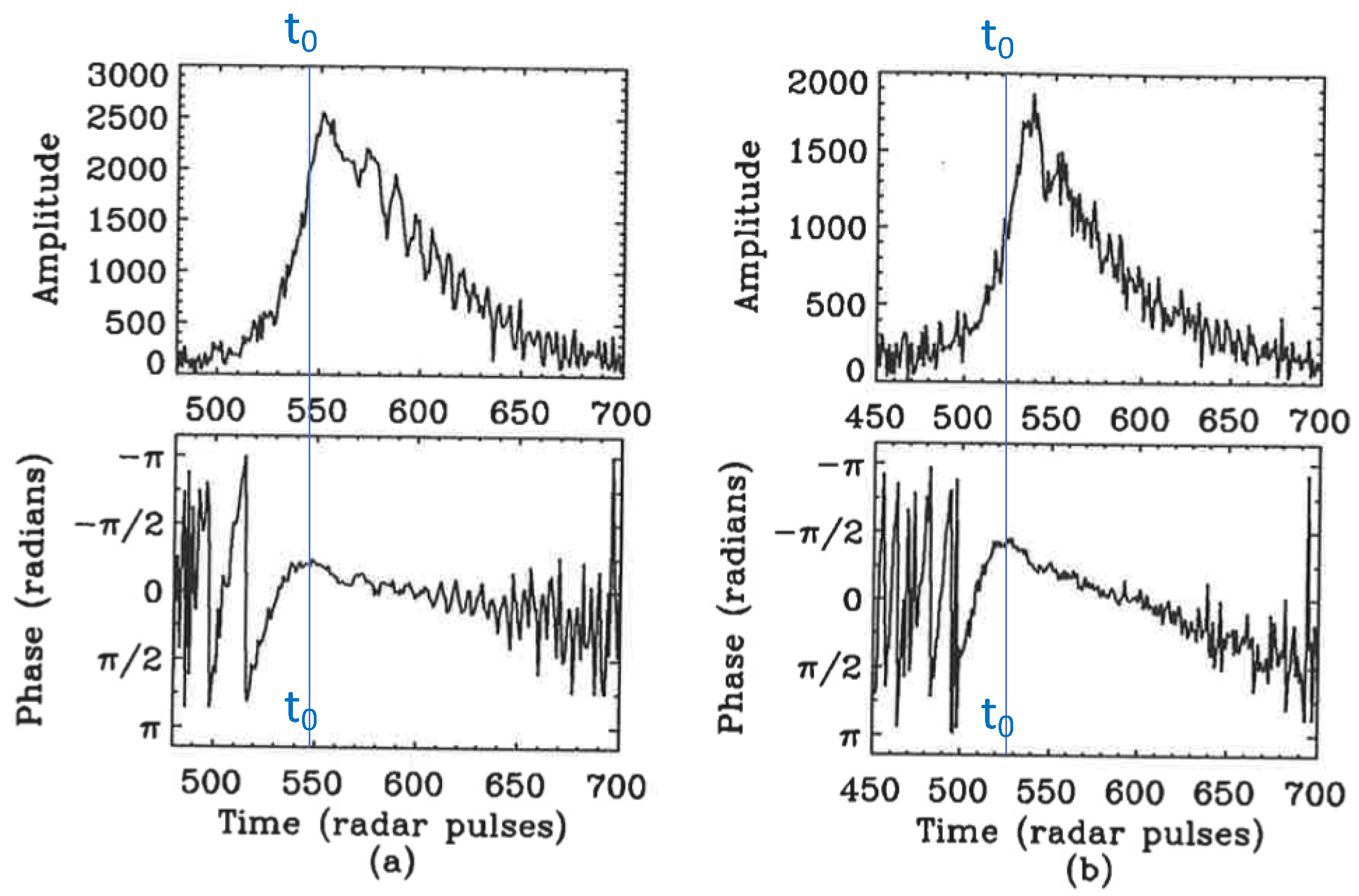
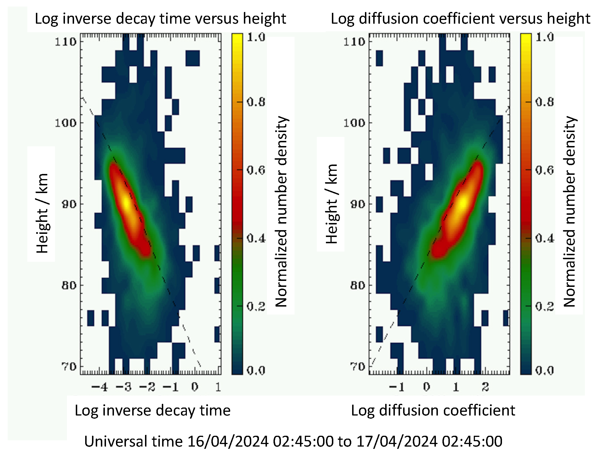
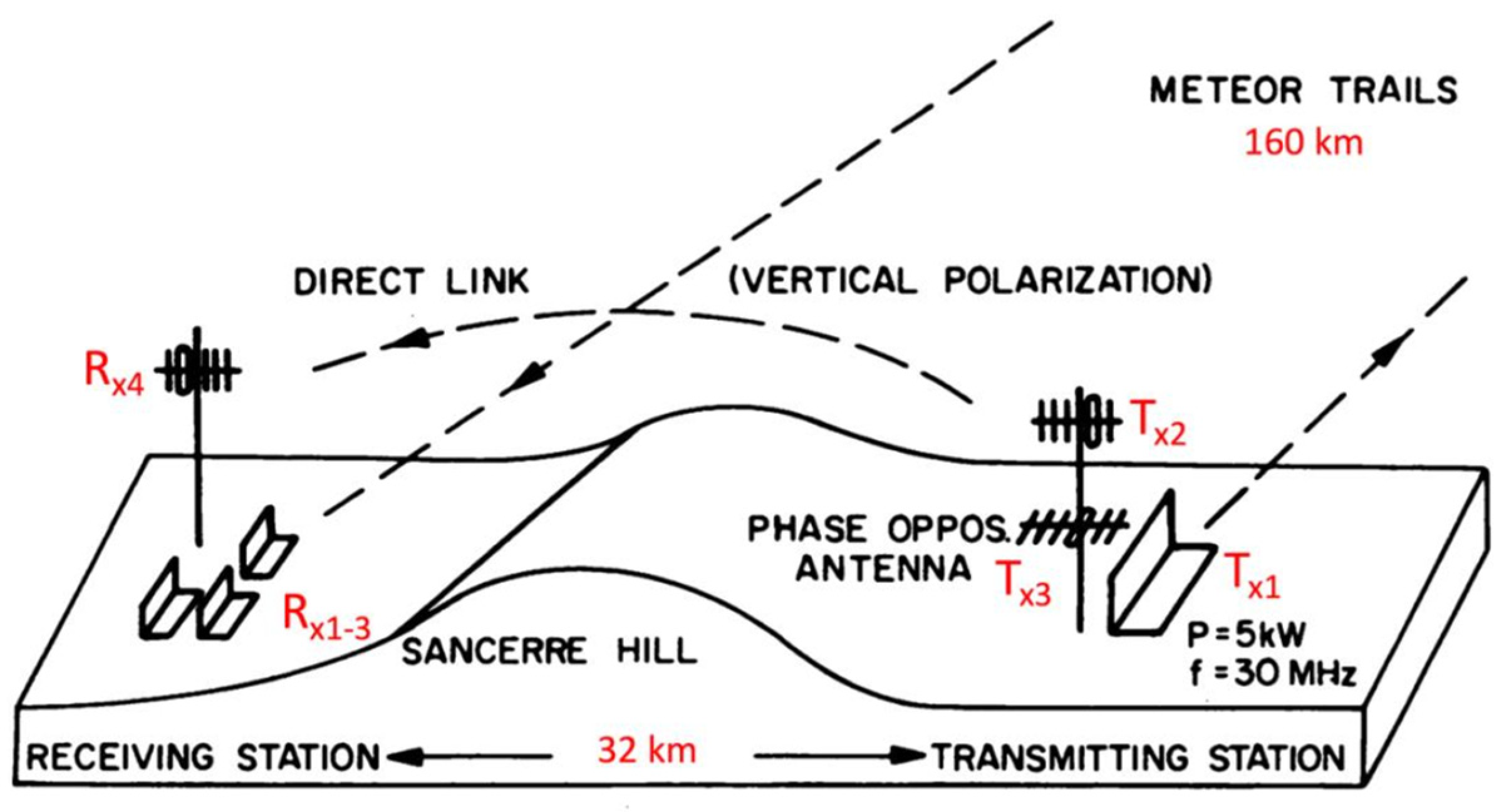
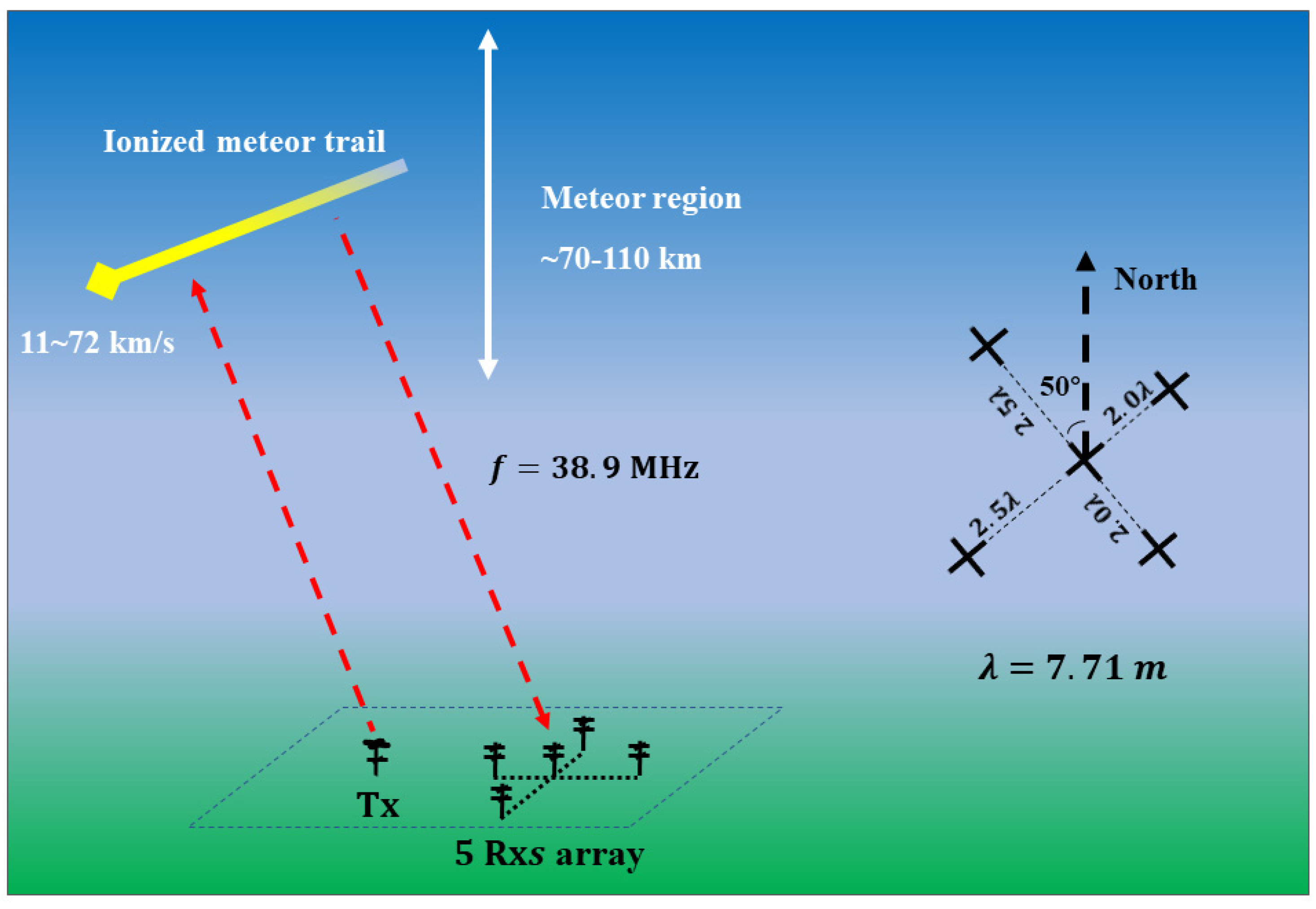
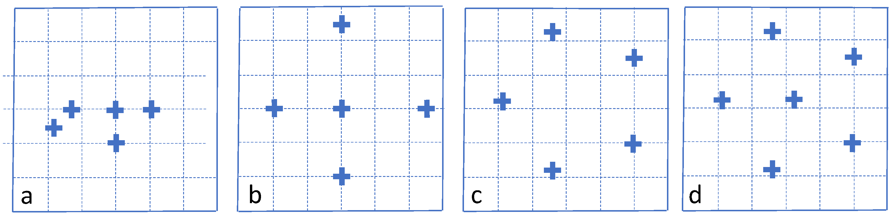
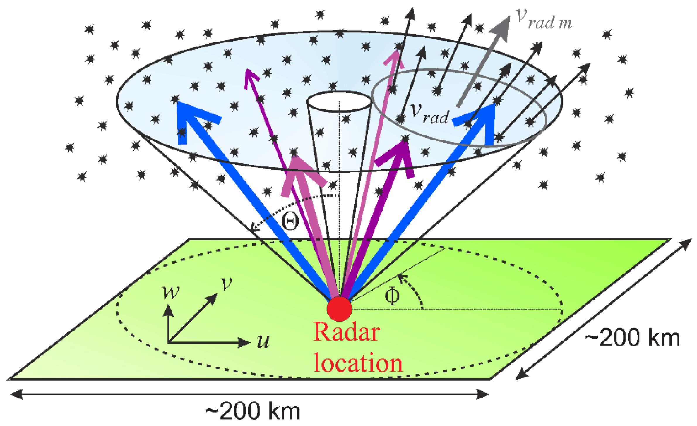
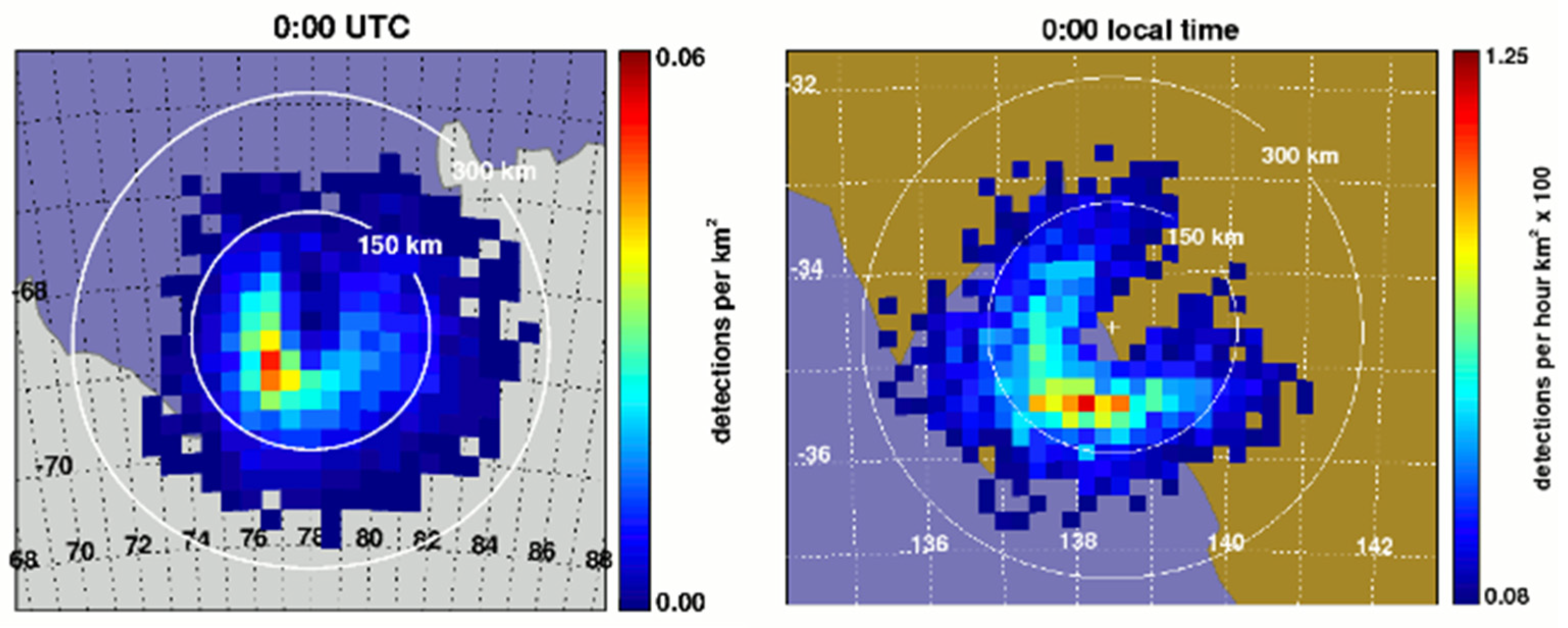
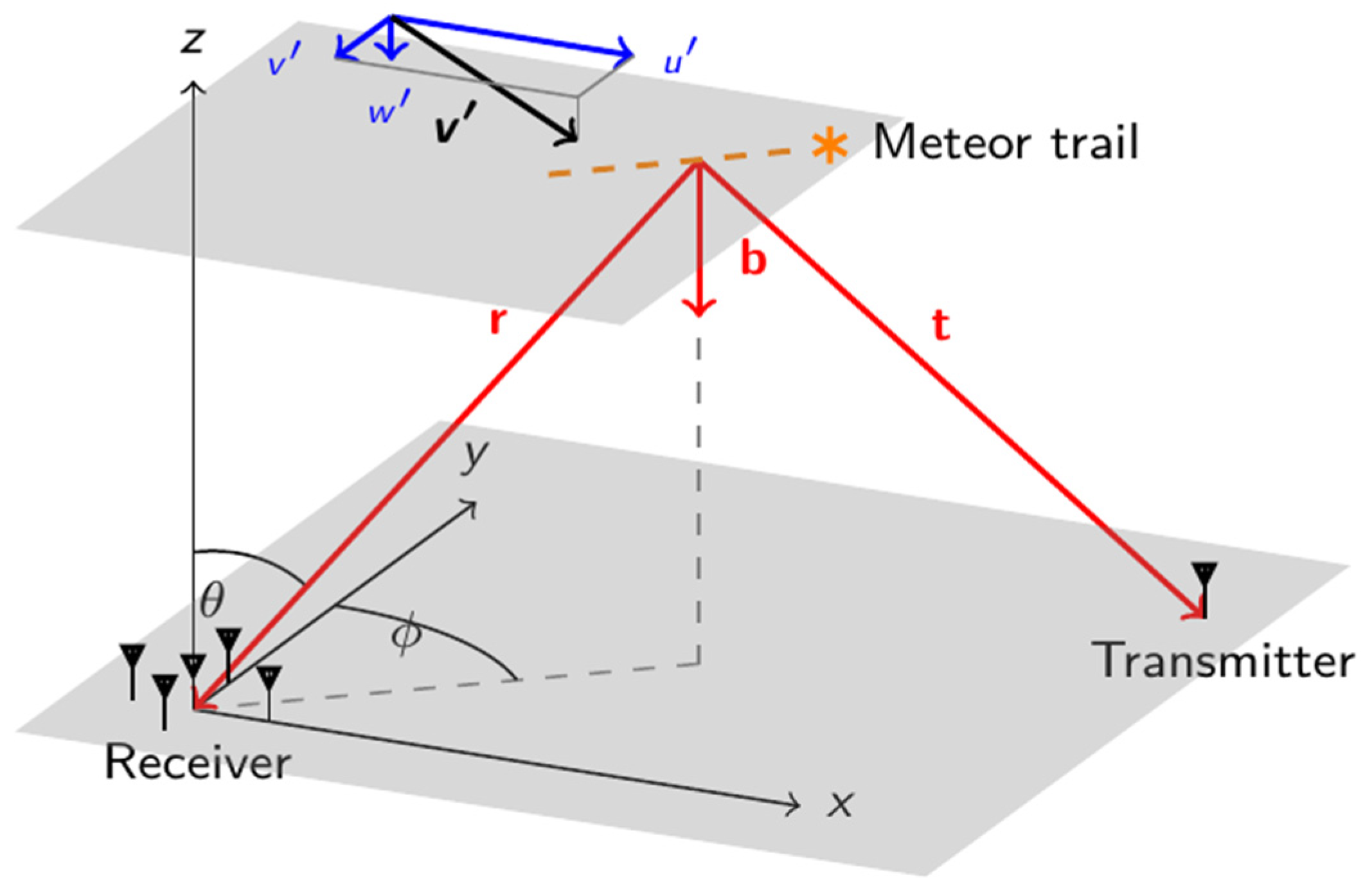
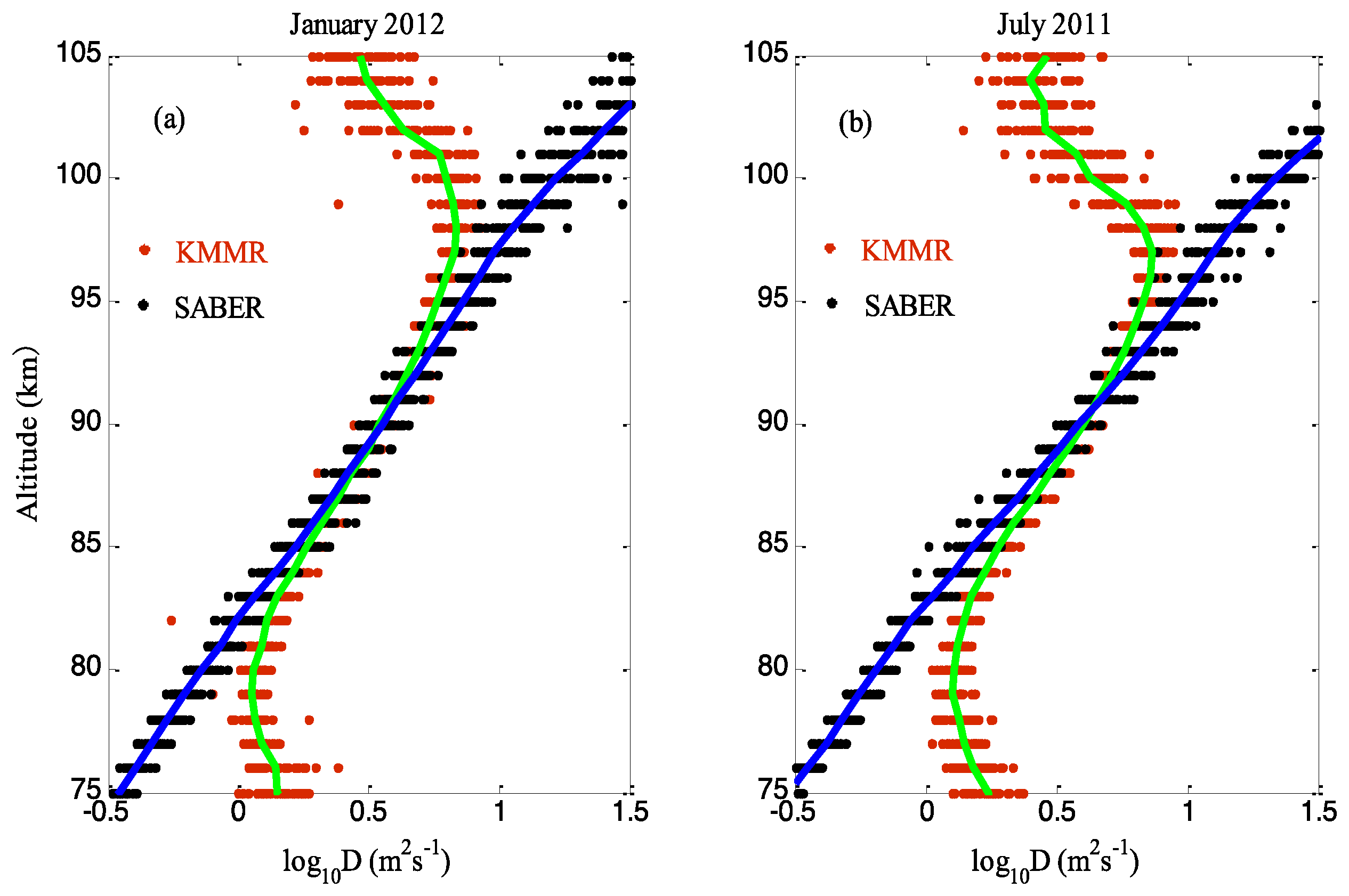
Table 1.
The main operational parameters of two modern meteor radars. Mengcheng is a dedicated all-sky meteor radar; Langfang is an all-sky meteor radar that shares the same ST hardware but uses its own transmitting and receiving antennas. It is unique in that the ST and meteor radars have separate operating frequencies for the two modes.
| Parameter | Mengcheng [80] | Langfang [85] |
|---|---|---|
| Location | USTC Observatory, Mengcheng (33.4° N, 116.5° E), China | NSSC Langfang Observatory (39.39° N, 116.66° E), China |
| Frequency | 38.9 MHz | 35.0 MHz in Meteor Mode; 53.8 MHz in ST Mode |
| Receive Channels | Six (Five used) | Six (Five used); Six (One used) |
| Peak power | 24 kW | 48 kW |
| Antennas | One crossed two-element folded dipole for Tx, and five two-element crossed Yagis for Rx | One crossed two-element folded dipole for Tx, and five two-element crossed Yagis for Rx; 144 (12 × 12) three-element linear Yagis for Tx/Rx, tuned |
| Pulse repetition frequency | 430 Hz | 430 Hz; user selected |
| Transmission mode | Circular | Circular; linear |
| Coherent integrations | Four | Four; user-selected |
| Range resolution | 1.8 km | 1.8 km; from 100 m |
| Pulse type | Gaussian | Gaussian; Raised cosine |
| Pulse width | 24 μs | 24 μs; user-selected |
| Duty cycle | 8.3% | 8.3%; 2.4% @ 600 m |
| Detection range | 70–110 km | 70–110 km; 0.5–20 km |
Disclaimer/Publisher’s Note: The statements, opinions and data contained in all publications are solely those of the individual author(s) and contributor(s) and not of MDPI and/or the editor(s). MDPI and/or the editor(s) disclaim responsibility for any injury to people or property resulting from any ideas, methods, instructions or products referred to in the content. |
© 2024 by the author. Licensee MDPI, Basel, Switzerland. This article is an open access article distributed under the terms and conditions of the Creative Commons Attribution (CC BY) license (https://creativecommons.org/licenses/by/4.0/).
Share and Cite
MDPI and ACS Style
Reid, I.M. Meteor Radar for Investigation of the MLT Region: A Review. Atmosphere 2024, 15, 505. https://doi.org/10.3390/atmos15040505
AMA Style
Reid IM. Meteor Radar for Investigation of the MLT Region: A Review. Atmosphere. 2024; 15(4):505. https://doi.org/10.3390/atmos15040505
Chicago/Turabian StyleReid, Iain M. 2024. "Meteor Radar for Investigation of the MLT Region: A Review" Atmosphere 15, no. 4: 505. https://doi.org/10.3390/atmos15040505
Note that from the first issue of 2016, this journal uses article numbers instead of page numbers. See further details here.