Article

A Climatological Study of Western Mediterranean Medicanes in Numerical Simulations with Explicit and Parameterized Convection

1
Department of Earth and Environmental Sciences, University of Milan-Bicocca, 20126 Milan, Italy
2
Laboratoire de Physique, ENS de Lyon, Université Claude Bernard, 69364 Lyon, France
3
CIMA Foundation, 17100 Savona, Italy
4
Institute of Atmospheric Sciences and Climate, Consiglio Nazionale delle Ricerche (ISAC-CNR), 10133 Turin, Italy
*
Author to whom correspondence should be addressed.
Atmosphere 2018, 9(10), 397; https://doi.org/10.3390/atmos9100397
Submission received: 31 July 2018 / Revised: 27 September 2018 / Accepted: 2 October 2018 / Published: 11 October 2018
(This article belongs to the Special Issue Mediterranean Tropical-Like Cyclones (Medicanes))

Abstract

:
The semi-enclosed Mediterranean basin, surrounded by high mountains, is placed in a favorable location for cyclonic storms development. Most of these are extratropical cyclones of baroclinic and orographic origin, but occasionally, some low pressure systems may develop to assume features characteristic of tropical cyclones. Medicanes (MEDIterranean hurriCANES) are infrequent and small-sized tropical-like cyclones. They originate and develop over sea, and are associated with strong winds and heavy precipitations. Proper definitions and classifications for Medicanes are still partially lacking, and systematic climatic studies have appeared only in recent years. In this work, we provide climatologies of Medicanes in the Western Mediterranean basin based on multidecadal runs performed with the Weather Research and Forecasting regional model with different resolutions and setups. The detection of Medicanes is based on a cyclone tracking algorithm and on the methodology of Hart cyclone phase space diagrams. We compare the statistics of Medicanes in the historical period 1979–1998 between runs at a resolution of 11 km with different convective parameterizations and microphysics schemes and one run at a resolution of 4 km with explicitly resolved convection. We show how different convective parameterization schemes lead to different statistics of Medicanes, while the use of different microphysical schemes impacts the length of the cyclone trajectories.

1. Introduction

The semi-enclosed Mediterranean basin is one of the main cyclogenesis regions in the world [1]. Most cyclones developing in the area have baroclinic or orographic origin. Due to thermodynamic disequilibrium, occasionally, some of them evolve into warm core cyclones undergoing a tropical transition [2]. Medicanes, a contraction of MEDIterranean HurriCANES, or Mediterranean tropical-like cyclones (TLC), are mesoscale storms characterized by warm sea surface temperatures of at least 15 °C and baroclinic cut-off lows in the upper atmospheric layers [2,3,4,5]. The enthalpy transfer at the air–sea interface is essential for the environmental imbalance and promotes deep convection and tropopause divergence. Medicanes are not tropical cyclones in a strict sense. They are low pressure systems that typically form as classical extratropical baroclinic low pressure systems and then evolve into roughly axisymmetric structures, with an eye surrounded by an eyewall, that, at least in their mature phase, are maintained the same way as tropical cyclones, by inducing large enthalpy fluxes from the sea [2].
As revealed by satellite images, Medicanes have a spirally shaped cloud cover with a clear circular eye in the middle, surrounded by an eyewall [6]. In the mature stage, they can assume the same structure and properties of tropical cyclones, but are of a smaller size. The spatial scale of a Medicane never extends beyond a diameter of 300 km, with a lifetime from 12 h to 5 days for a track between 700 and 3000 km. Seasonal distribution is characterized by a very low number of events in summer, a high activity during autumn, and a flattish tail in winter and spring [7,8,9]. In most cases, TLCs maintain tropical features for less than 24 h, reaching a maximum wind intensity of about 30 m/s, with gusts above 40 m/s, corresponding to the lower bound of the hurricane category 1 on the Saffir–Simpson scale.
Since the 1980s, several studies have been carried out based on satellite images or by combining models and observations. Early studies focused on structural features such as the vertical wind profile, the temperature fields and the amount of precipitation [10,11,12,13]. Other studies focused on the role played by heat fluxes in the development of Medicanes [2,3,5,6,11,14,15]. The atmospheric environment is analyzed, for example, in [4,16].
The lack of observations over sea, the episodic occurrence of Medicanes and the small size make it difficult to recognize the meteorological features associated with them [6]. There is not a clearcut distinction between Medicanes and the broad spectrum of Mediterranean low-pressure systems. A significant fraction of Medicanes look like hybrid cyclonic storms combining, in different proportions, the physical mechanisms of ordinary extratropical (e.g., frontal dynamics) and tropical disturbances [17]. These hybrid systems have only a weak lower-tropospheric, warm-core structure resulting from the lack of sustained convection near the cyclone centre [2]. A minimal necessary condition that is generally accepted for the development of a Medicane is the presence of a warm core in the lower troposphere. Other criteria are more debatable but some ideal candidates have been identified, such as the presence of a warm core in the upper tropospheric layer.
Several methods have been developed for the detection of Mediterranean cyclones from numerical models. An identification procedure to investigate the sea level pressure field was proposed by [18,19], at first without discriminating among tropical and extratropical features, and later specifically for mesoscale cyclones. An algorithm for the identification of Mediterranean cyclones was implemented by [6]. Climatologies of Medicanes based on 60 years simulations at different resolutions were provided by [8]. Recently, ref. [20] performed an analysis in the context of the MedCORDEX and EURO-CORDEX projects. Note, however, that a general difficulty in performing statistical analyses of Medicanes is presented by the fact that a universally accepted definition of Medicanes is still lacking.
Previous climatological studies were based on numerical simulations with relatively coarse resolution (25–40 km), and are thus at the edge of reliability to study small scale structures like Medicanes. To assess the robustness of those studies, it is therefore of importance to investigate the effects of different representations of small scale processes (crucially, moist processes, that is, convection and cloud microphysics) on the statistical properties of Medicanes. In this study, we analyze multidecadal simulations obtained with the Weather Research and Forecast model (WRF) over the Western Mediterranean with different setups, parameterization schemes, and grid spacings from about 4 km to about 11 km. We then apply the cyclone tracking method of [18,19] and the Medicane identification method of [21] to create climatologies of Medicanes and of their thermal properties.
The paper is structured as follows. In Section 2, we describe the set of simulations analyzed for this study, and how we have adapted tracking and identification methods commonly used in the literature to our analysis. In Section 3, we describe the results of the analysis. First, we perform some sensitivity tests on parameters of the tracking and identification methods, to assess the robustness of the procedure. Then, we analyze the dependence of the present day statistics of Medicanes on the representation of convection in the model. We compare a high resolution, non-hydrostatic, convection permitting simulation, with slightly coarser runs with parameterized convection. We consider three runs with parameterized convection, making use of different convective schemes and microphysics. All the simulations are forced by reanalysis data. In Section 4, we summarize the main outcomes of this work and discuss possible developments.

2. Materials and Methods
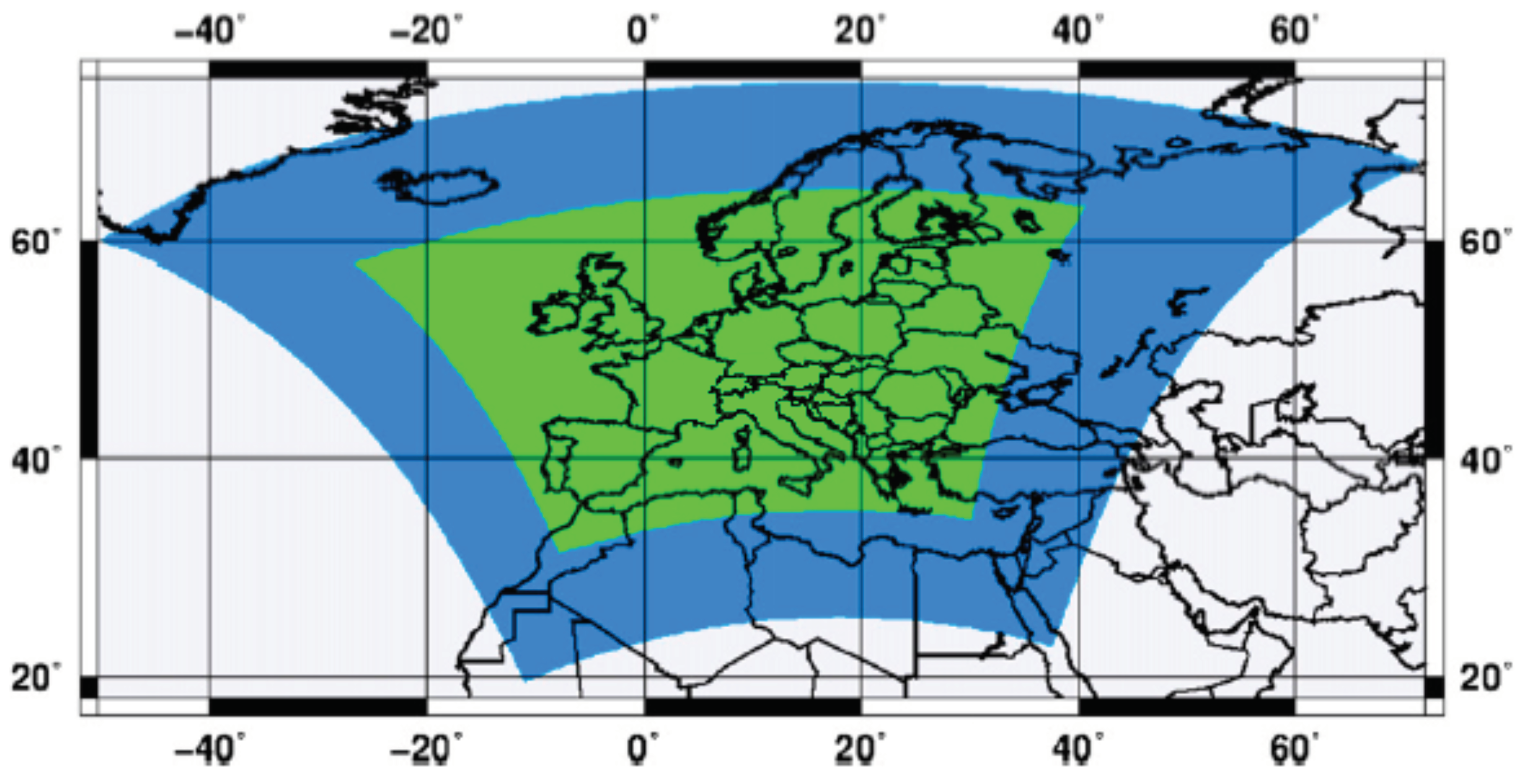
2.1. Data

Data for the present study are the 3 hourly output of simulations performed with the Advanced Research version 3.4.1 of the Weather Research Forecast regional model as part of a previous project (EXPRESS-Hydro, Pieri et al. [22]). One run (named et04 in the following) was performed in a non-hydrostatic setup with a spatial resolution of 0.037° (about 4 km) for the period 1979–2008 (Table 1). The boundary and initial conditions were provided by ERA-Interim data. In order to avoid abrupt resolution change with respect to the forcing dataset, a two-way nesting strategy was used. The model was run at 0.11° (approximately 11 km) in a wider domain (the EURO-CORDEX domain shown in blue in Figure 1), and at 0.037° (approximately 4 km) in the internal domain (shown in green in Figure 1). In the external domain, the Kain–Fritsch convective scheme was used. See [22] for more details.
Furthermore, several multidecadal runs were performed at a spatial resolution of 0.11° over the EURO-CORDEX domain with different convective parameterizations and microphysics schemes. In this study, we consider three historical simulations run with ERA-Interim boundary conditions for the period 1979–1998. The historical run kt11 was performed with the Kain–Fritsch (KF) convection scheme [23] and the Thompson microphysics scheme [24]. The historical run kw11 was performed with the KF convection scheme and with the WRF Single Moment 6 (WSM6) microphysics scheme [25]. The historical run bt11 was performed with the Betts–Miller–Janjic (BMJ) convection scheme [26] and the Thompson microphysics scheme.
The different setups chosen in this study are expected to lead to different results. Recent studies have shown that WRF shows high sensitivity to the choice of parameterization layout in the statistics of tropical cyclones [27] and in the properties of Medicanes [28]. In a previous study [22], the precipitation data from the same simulations used in our study were compared with several observational products. While a good overall agreement between observed and modeled precipitation patterns was found, the model outputs displayed a positive precipitation bias, and this was dependent on the representation of convection. Explicitly resolved convection was shown to considerably reduce precipitation biases in summer, and differences existed among the different convective parameterization schemes, with BMJ outperforming the KF scheme, but underestimating the probability of extreme precipitation rates.
The KF parameterization is a mass-flux scheme that is suitable for mesoscale models and able to handle very intense convection. BMJ, on the other hand, is a profile-relaxation-type scheme that adjusts the sounding toward a reference profile derived from climatology. The non-hydrostatic run is supposed to have the best skills in capturing the details of the convective processes involved in the initiation and development of a Medicane. Differences in the microphysics scheme have also been shown to impact the simulations of case study Medicanes [29,30]. In this work, we tested two microphysics schemes. The WSM6 scheme [25] has six prognostic water substance variables, and each hydrometeor distribution is fully determined by the specification of the mixing ratio of the corresponding hydrometeor species (single moment). The [24] microphysics scheme is a two-moment scheme as it also predicts number concentrations for ice and rain based on the environmental conditions.
Different areas of cyclogenesis are present in the Western and Eastern parts of the Mediterranean basin [31,32,33]. In our simulations, the domain of the high resolution run covers the Mediterranean sea only partially (Figure 1). The Eastern Mediterranean is partially excluded from the domain and the Central Mediterranean is crossed by the boundaries of the internal domain. Border effects due to change in resolution in the nesting procedure could affect the results on the statistics. Since, in this study, we are particularly interested in comparing the statistics of runs with parameterized convection with those of the run with high resolution explicit convection, we limit the analysis of the statistics of Medicanes to an area comprised between 5° W–20° E longitude and 35° N–46° N latitude. This includes the Western Mediterranean and a part of the Central Mediterranean. In the following, we call this area Western Mediterranean (WM) for simplicity.
It is important to clarify that we take the high resolution non-hydrostatic run as a reference from the point of view of the precision of the representation of the physical processes involved, but we do not claim that this is an exact representation of reality. Given the way the simulations are set up, even a perfect numerical model would not lead to a punctual, one to one correspondence with what happened in the real world. The frequency and characteristics of Medicanes should match the real ones, but we do not expect to recreate exactly a given storm occurring at a given place on a given date, as the reanalysis data only prescribe the boundary conditions in the EURO-CORDEX domain, and this is not sufficient to determine the inner evolution of the perturbations. The transition of the synoptic scale cyclones into TLC and their subsequent evolution depend on many circumstances at the local scale, which can differ between reality and simulations. This work is thus strictly statistical in nature. Note that, in general, a comparison with observations is quite difficult, since, as explained in the next session, the detection of Medicanes requires information on the vertical thermal structure of the cyclones. Pure observational data are thus not available for a climatological study, and reanalysis data have a resolution that is probably too coarse to provide a reliable representation of Medicanes.

2.2. Methods

The analysis of the Medicane activity is divided into two parts. First a cyclone tracking algorithm is applied to preselect cyclone trajectories which are potential candidates to have evolved into Medicanes during their evolution. The tracking algorithm is adapted from a standard method for tracking extratropical cyclones [18] and then modified to capture smaller mesoscale cyclones [19]. Once a dataset of potential trajectories has been obtained, the Hart criteria for detecting warm core cyclones is applied to each instant of the trajectories [21]. In the following, we describe the two methods.

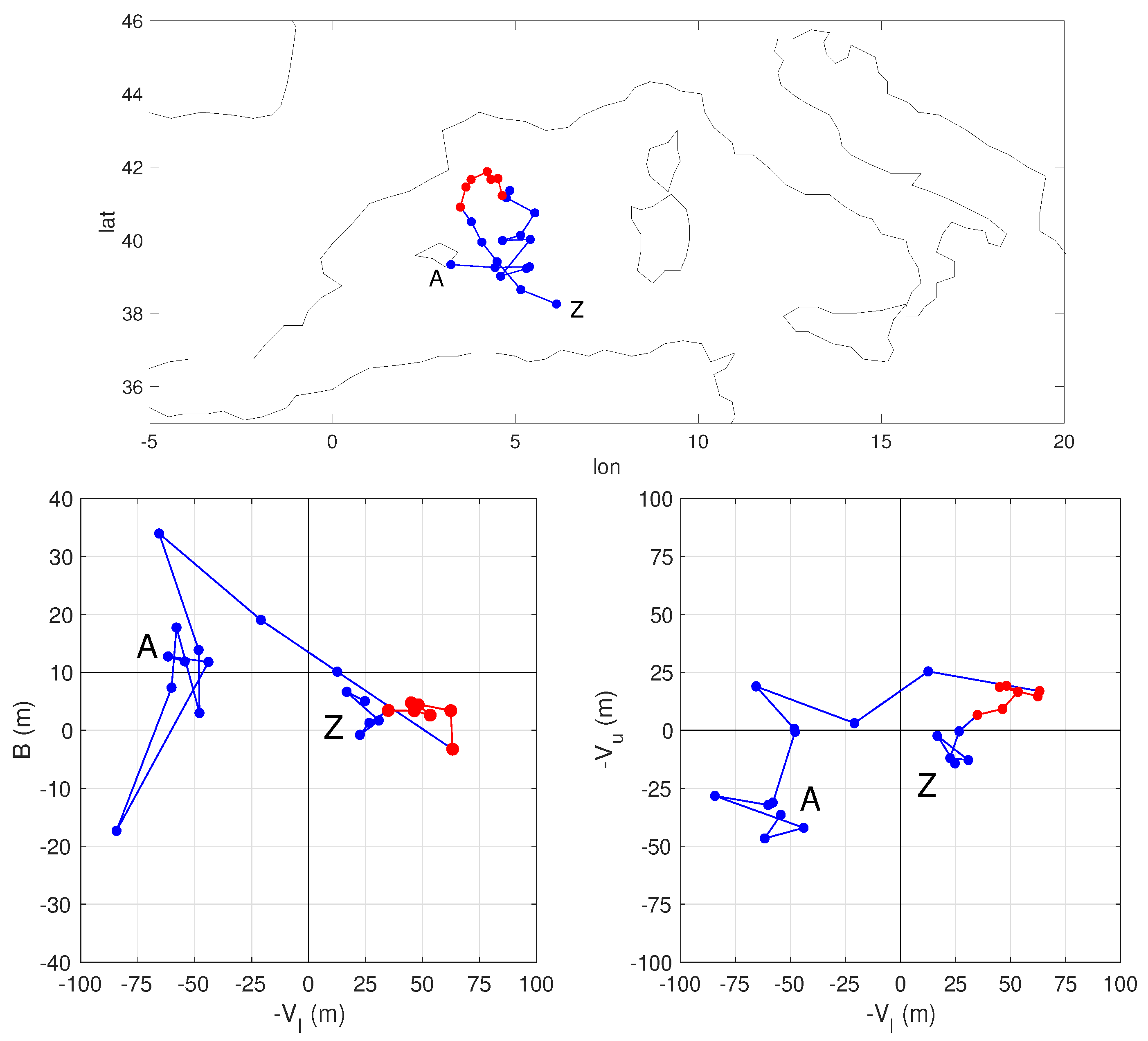
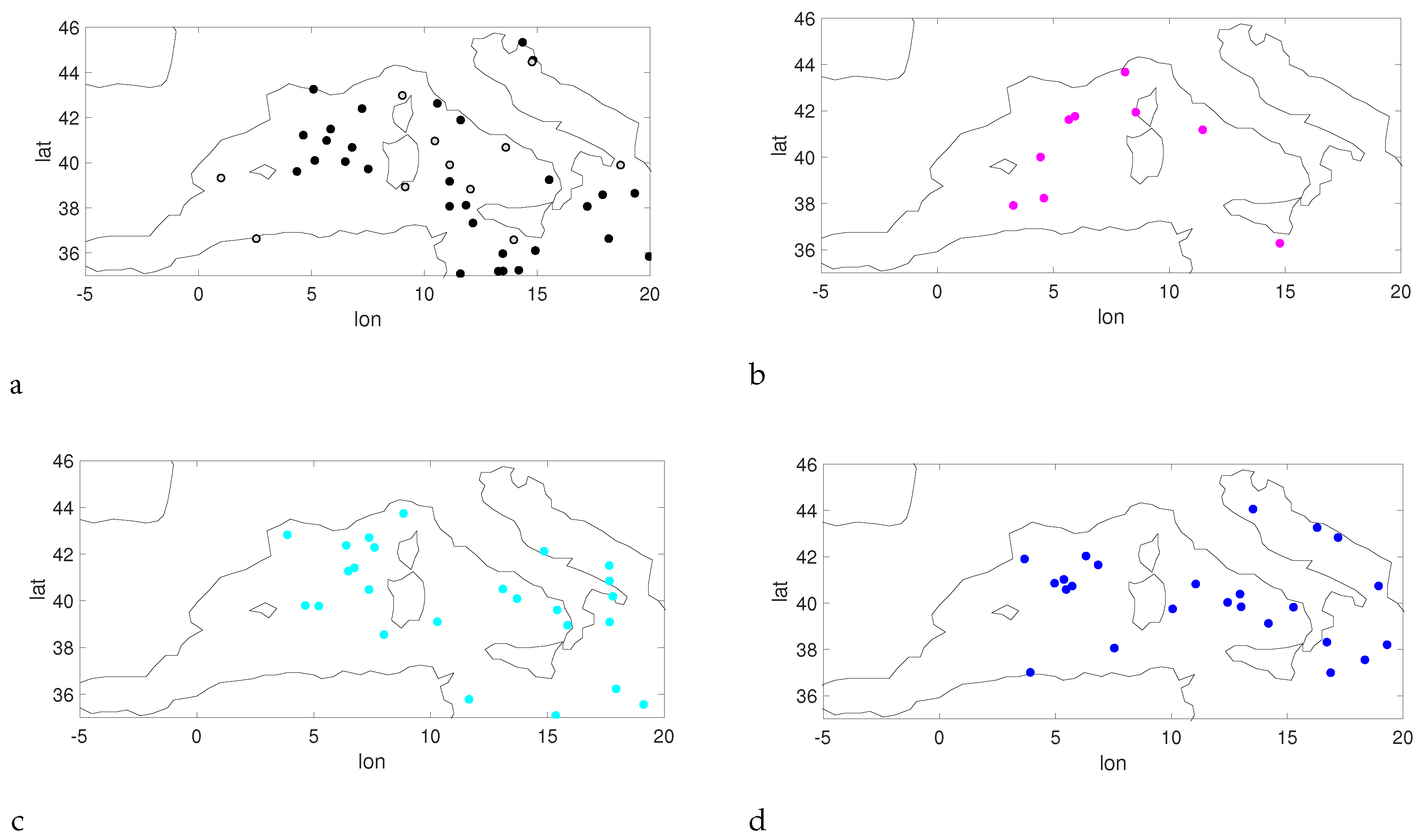
2.2.1. Cyclone Tracking

The cyclone tracking method is similar to [18,19]. The algorithm first looks for local minima in the instantaneous sea level pressure field. Then, a selection is applied on the set of minima in order to keep only minima corresponding to structures strong enough. The selection is based on the values of the sea level pressure gradient around the minimum. Once the strong minima are selected, a proximity criterion is applied in order to connect minima at successive time instants in order to build cyclone trajectories.
First of all, a spatial Cressman filter [34] is applied to the sea level pressure in order to remove local minima due to the noisy nature of the field, and to identify only those related to real mesoscale dynamical structures. The filtered sea level pressure p ˜ s x , t at grid point x and time t is obtained taking a weighted average of the original sea level pressure p s x , t on a circular area A of radius D around x
p ˜ s x , t = A W x , x p s x , t d A A W x , x d A ,
where the weighting factor W x , x depends on the distance d x , x between x and its neighbors x
W x , x = D 2 d 2 x , x D 2 + d 2 x , x .
Local minima on the field of the filtered pressure are then recorded. In the original formulation of the tracking algorithm [18], designed for the detection of large scale extratropical cyclones, the influence radius in the Cressman filter was D = 200 km. In order to preserve smaller structures like Medicanes, we set the radius to D = 50 km, as in [19].
For each minimum, we then compute the gradient of the sea level pressure along the eight principal directions (E, NE, N, NW, W, SW, S, SE) inside a circle of radius 300 km. Since the grid of the model is not regular, the pressure field is interpolated along each of the eight directions over a set of equidistant points 10 km from each other. For each direction, we take the maximum sea level pressure gradient. The minimum is classified as the centre of a potentially interesting cyclone if the sea level pressure gradient is larger than a threshold G along at least N of the eight principal directions. In [19], the criteria were N = 6 and G = 3.21 10 2 hPa km 1 . However, we noticed that the threshold value of G = 3.21 10 2 hPa km 1 in at least N = 6 directions is a very strong requirement which creates problems in the detection of cyclones. In fact, it happens relatively often that a minimum in the middle of a trajectory goes below the threshold, making our automated tracking algorithm split the trajectory in two or more parts, eventually losing it for the following analysis of Medicanes, which require a minimum length of the trajectories. We have therefore chosen to use the lower threshold G = 0.5 10 2 hPa km 1 (previously used in [18] to detect extratropical cyclones) in at least N = 6 directions in this first phase. The requirement of a stronger intensity of the cyclones is then applied later, after the trajectories have been reconstructed, as explained in the following.
Once the minima at each time instant have been selected, a proximity condition is imposed in order to reconstruct the trajectories. Starting from time t = 0 , for each minimum at time t, we check if there is a minimum at time t + Δ t which is closer than Δ x = V Δ t , with V = 50 km h 1 and Δ t = 3 h. In that case, the two minima are considered to belong to the same trajectory. We verified that thanks to the filtering and the selection described above, no inconsistencies (for example, two minima at time t + Δ t both possible successors of one single minimum at time t) were found.
Once the trajectories have been classified, further conditions are imposed in order to preselect only the ones which are relevant for our analysis. All the trajectories shorter than 24 h are discarded. All the trajectories that spend less than 12 h over sea are discarded. If a trajectory spends at least half of its life over land or at less than 100 km from the coast, it is discarded unless it has moved for at least 1000 km during its lifetime (this removes quasi-stationary minima due to orographic effects close to the coastlines). Finally, the condition on the intensity of the minima is applied. We keep all the trajectories for which the maximum of the gradient is larger than a threshold G = 3.21 10 2 hPa km 1 in at least N = 6 principal directions for at least 8 time steps that are not necessarily consecutive. We performed a sensitivity study on the value of G and found that the value G = 3.21 10 2 hPa km 1 used in the literature gives consistent results also in our case.

2.2.2. Medicane Identification

An accepted precise definition of Medicanes is still lacking. The scientific community is currently discussing the criteria that should be met in order to classify a cyclonic perturbation as a Medicane, i.e., a tropical-like cyclone in the Mediterranean region, but there is a substantial agreement on the fact that the main difference with respect to classical extratropical cyclones relies upon the existence of a warm core (Lluìs Fita Borrell, personal communication). Here, we adopt a method for characterizing cyclones developed by [21]. Three parameters are used to represent the thermal structure of a cyclone. The parameters are computed using the geopotential height field Z at three different vertical levels within a circle of radius 100 km around the cyclone centre. The three parameters are:
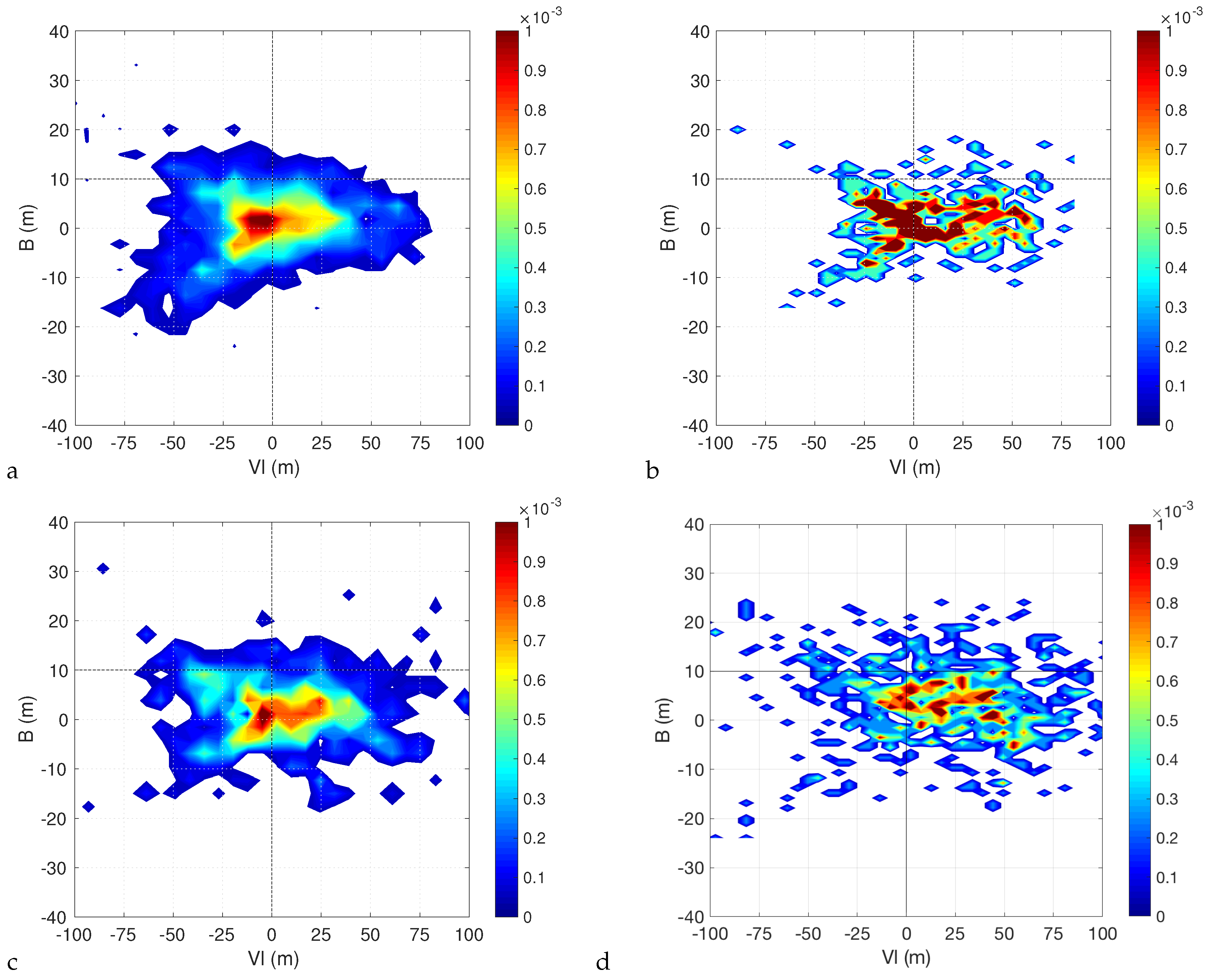
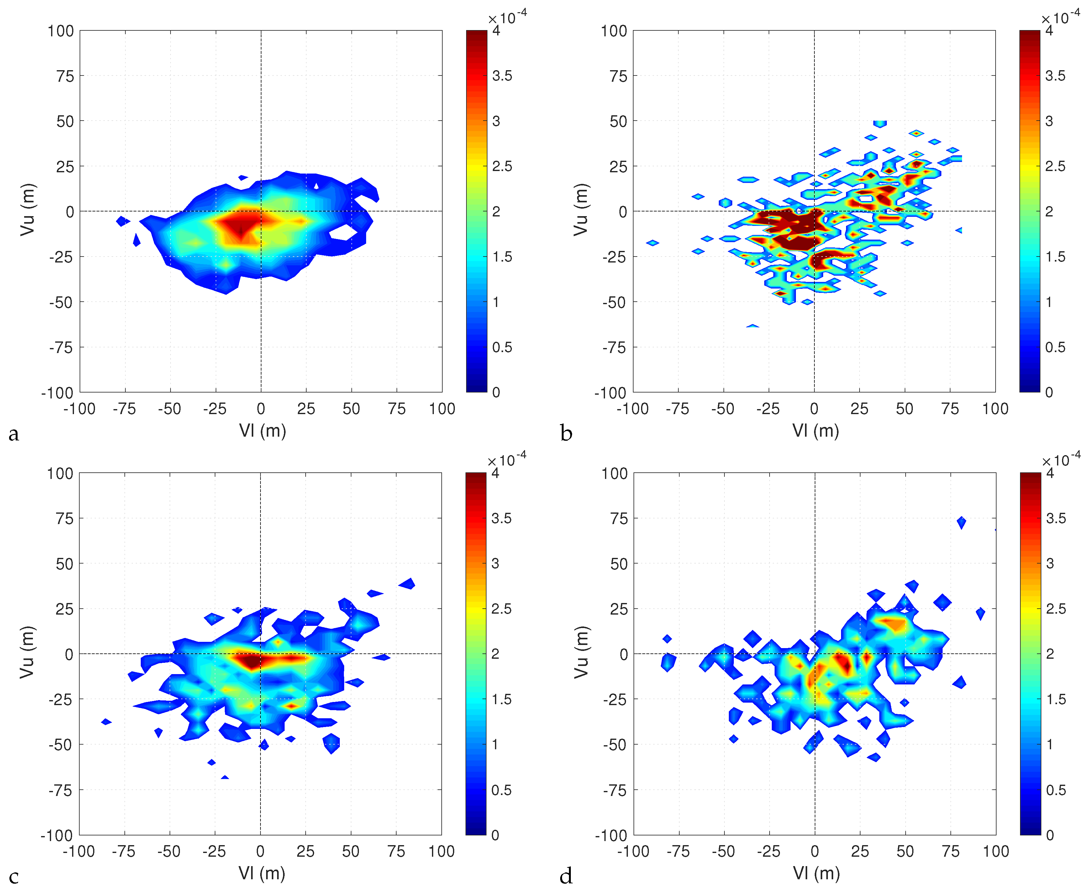
  • B, a measure of the thermal asymmetry of the cyclone in the lower troposphere, defined as the difference in mean thickness between the 850 hPa and 500 hPa isobaric surfaces at the right and left of the cyclone trajectory
    B = Z 500 x , t Z 850 x , t ¯ R Z 500 x , t Z 850 x , t ¯ L
    where the overbar indicates the mean over the area of a semicircle of radius 100 km, located to the right (subscript R) or to the left (subscript L) of the storm trajectory.
  • V l , a measure of the lower tropospheric thermal wind. By defining Δ Z = m a x ( Z ) m i n ( Z ) (where the maximum and the minimum are taken at the same pressure level), V l is defined as
    V l = Δ Z ln ( p ) 850 500 ;
  • V u , a measure of the upper tropospheric thermal wind, which is similarly defined as
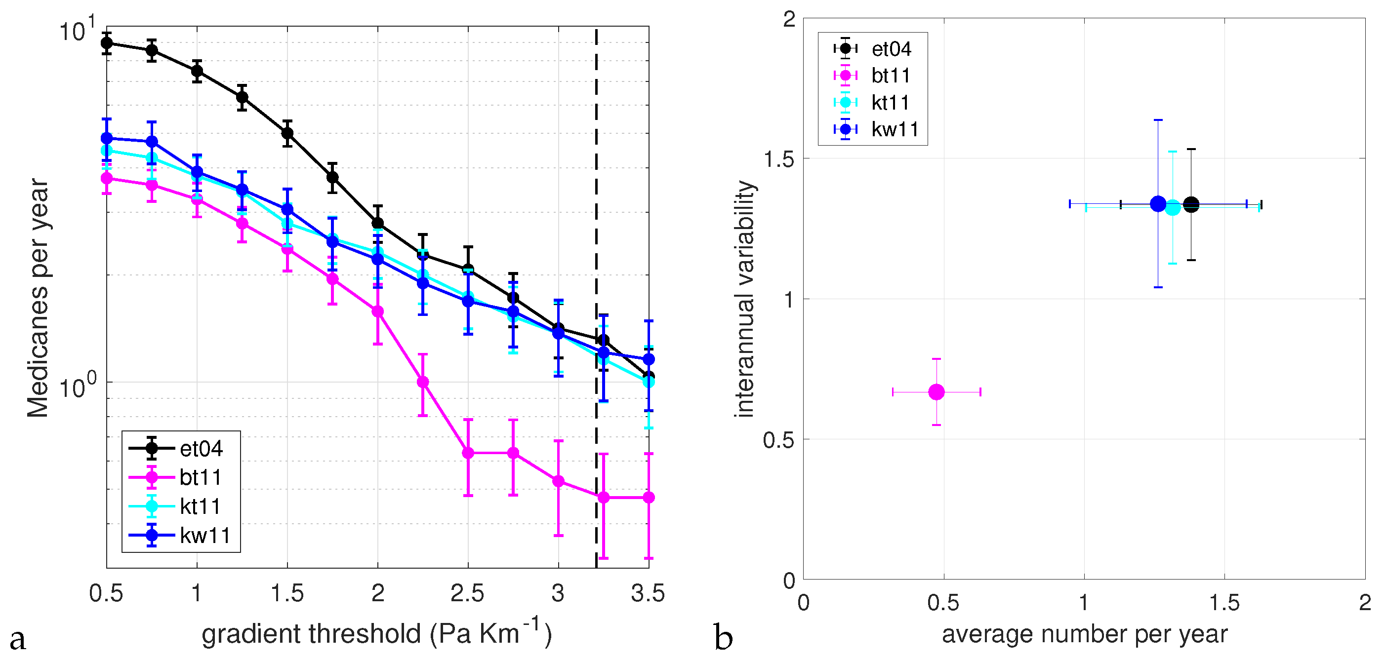
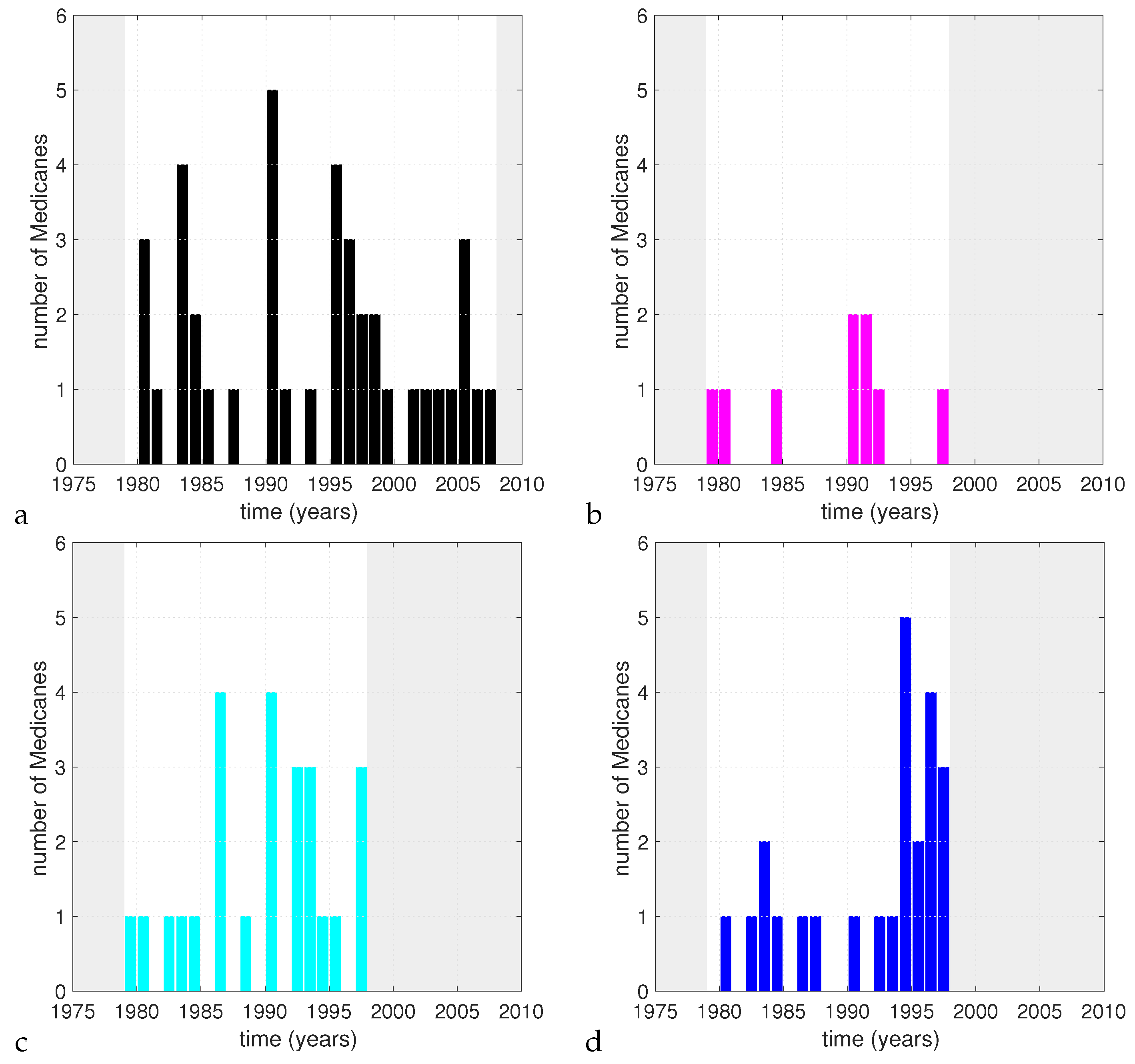
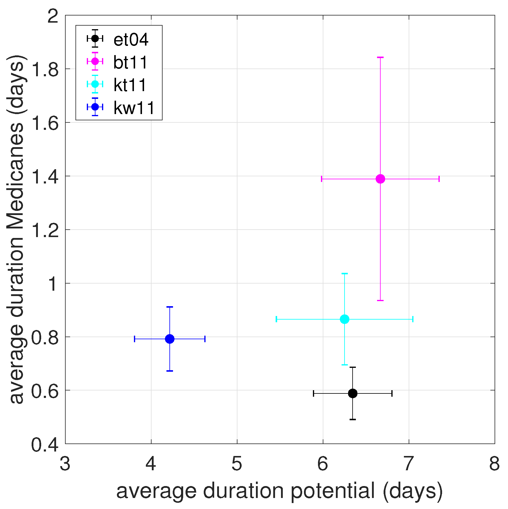
    V u = Δ Z ln ( p ) 500 200 .
In Hart’s view, a tropical or tropical-like cyclone is a non-frontal system characterized by thermal symmetry, while an extratropical cyclone is a frontal system that is thermally asymmetric. Mature tropical cyclones have values of B of approximately zero, while developing extratropical cyclones have large positive values of B. The condition for distinguishing a tropical thermal gradient from a non-tropical thermal gradient is conventionally set at B < 10 m [21,35]. The parameters V l and V u instead describe the cold vs warm core vertical structure of the cyclone. See Appendix A for a discussion on their derivation. Positive (negative) values of V l indicate a cyclone with a warm (cold) core in the lower troposphere, and equivalently for V u and the upper troposphere [21]. Tropical and extratropical cyclones have warm and cold cores, respectively, throughout the whole troposphere. Hybrid and transitioning cyclones may have different signs for the thermal wind parameters. Here, we define a Medicane as a cyclone with B < 10 and with V l > 0 and V u > 0 (that is, a deep warm core symmetric cyclone).
Note that, originally, ref. [21] used the isobaric surfaces of 900, 600 and 300 hPa. These values have been used in several other publications (e.g., [8,15,20,36]). Other authors have used different values, for example, ref. [19] used the isobaric surfaces at 925, 700 and 400 hPa. In our case, we used 850, 500 and 200 hPa (adapting the procedure for tropospheric layers of unequal mass), because the data available from the simulations only provided these three vertical levels. Our layers are higher than those used in the aforementioned publications. This will influence to some extent the numerical value of the parameters, but we do not expect this to change the statistics of the population of identified Medicanes substantially. The value of the threshold of 10 m for B is quite arbitrary, and it has been used in the literature both when using the 900–600 hPa layers and the 925–700 hPa layers. Moreover, in our study, the condition in the tracking algorithm about the surface pressure gradient being larger than a threshold along at least 6 directions around the centre already enforces a high degree of symmetry on the detected cyclones. Indeed, the B parameter is the least decisive in discriminating a detected potential cyclone from a Medicane. For what concerns the parameter V l , we expect that using the 850–500 hPa layers instead of the 900–600 hPa layers will change the value but not the sign of the parameter, and it is the latter that matters. The case of the parameter V u is more delicate, as temperature starts increasing with height at the tropopause and the 200 hPa level may already be in the stratosphere. In fact, ref. [19] suggest that for the Mediterranean, the upper layer for the Hart analysis can be lowered to 700–400 hPa, on the basis that in the midlatitudes, the tropopause is usually lower than in the tropics. Here, we cannot test how the algorithm is sensitive to the choice of the levels, as only 3 pressure level geopotential heights have been saved in the climatological simulations. We note that in the case of a classical extratropical cyclone, an upper layer that is too high may result in the spurious detection of a warm core if the 200 hPa pressure level is above the tropopause (see Figure 3b in [21]). By performing the analysis, we can say a posteriori that this rarely happens. On the other hand, we cannot rule out the possibility that the use of the layer 500–200 hPa sometimes leads to the unwanted attribution of a weak cold core anomaly where indeed a TLC is present, but numerical case studies of Medicanes showed that the temperature profile minimum is not lower than 200 hPa [15], proving that, at least in those cases, the use of the 500–200 hPa is appropriate.
Originally, ref. [21] used a radius of 500 km, which is too large for structures like Medicanes. In the literature on Medicanes, different radius values have been used. For example, refs. [19,36] used a variable radius whose value is computed by estimating the size of the warm core anomaly, while [8,15] used a fixed radius of 100 km after doing some testing on different parameter choices. Recently, ref. [20] used a fixed value of 150 km. Attempts to use a time dependent value have given poor performances [37], leading the authors to use a fixed value of 70 km. In this work, we used a radius of 100 km, as it has been found to be a good choice in several previous works [8,15], and as the results of case studies are not qualitatively sensitive to the precise value used [38].
Figure 2 shows an example of the Hart analysis for an individual cyclone from the non-hydrostatic run. The bottom panels of Figure 2 show the evolution in the three-dimensional Hart parameter space by two projections on the V l B (left) and V l V u (right) planes. The cyclone (blue) originated on 5 October 1996 close to the Balearic islands (A) as a normal extratropical cyclone characterized by thermal asymmetry ( B > 10 m) and both lower and upper cold cores ( V l < 0 m and V u < 0 m). In its evolution, it developed first an upper warm core and after some hours, at the beginning of 7 October 1996, transitioned to a full Medicane state (red in the figure) by acquiring also a lower warm core and pronounced thermal symmetry, while moving in the Northern part of the basin. The cyclone lost its Medicane status by the end of the same day by losing its upper warm core while moving south, and died as a hybrid cyclone close to the coast of North Africa on 8 October 1996 (Z).

3. Results

Medicane activity shows a marked seasonality (e.g., [8]). The number of events peaks in the autumn and winter, has high variability from February to July, and is very low in summer. Consequently, we compute the annual statistics of Medicanes not on the standard calendar year, but on a “Medicane year” extending from August to July of the following year, similarly to what was done in [8]. In the rest of the paper, when we talk about annual values or interannual variability, we refer to Medicane years. Note that in this way, for each dataset, the first 7 months of the first calendar year and the last 5 months of the last calendar year are excluded from the analysis.
A cyclone is classified as a Medicane if B < 10 m, V l > 0 m and V u > 0 for at least one time step. We performed a sensitivity study on the most critical parameter of the identification procedure, that is, the value of the threshold G on the intensity of the maxima of the sea level pressure gradient used to discard trajectories (after the cyclone trajectories have been reconstructed). We varied G between 0.5 × 10 2 hPa km 1 and 3.5 × 10 2 hPa km 1 . The lower value is the one used during the trajectory reconstruction step, that is, in that case, no further condition on the intensity of the cyclone is applied. Figure 3a shows the average number of Medicanes per year that were detected in the different historical runs as a function of G. Error bars were computed with bootstrap resampling. For each run, we calculated the time series of the annual number of Medicanes, and then we generated 10,000 series of the same length by random sampling with replacement from the initial one. The error bar is taken as the standard deviation of the distribution of average values obtained with the bootstrap. With this procedure, we take the simple hypothesis that the annual time series have zero or negligible time correlation. Although it is possible that some correlation on a multiannual scale exists, due to the NAO (Northern Atlantic Oscillation) or other climatic variability, or even on longer time scales, due to climate change, it is extremely hard to capture them on a sample of 20–30 years. Since no obvious correlation appears from the visual inspection of the time series, we have taken the simple approximation that they can be treated as uncorrelated. Even if they were, however, the effect on the estimate of the error would probably be small.
We can see that for values of G close to the one normally used in the literature (G = 3.21 × 10 2 hPa km 1 ), the non-hydrostatic run gives, on average, about 1.3–1.4 events per year, consistent with previous climatological studies [7,8]. Runs with the KF parameterization scheme agree very well with the non-hydrostatic run, giving values which are statistically indistinguishable, while the run with the BMJ parameterization scheme has much lower, more inconsistent values, below 0.5 events per year. For lower values of G, the run with the BMJ parameterization has values consistent with the runs with other parameterizations. The drop in the number of Medicanes with respect to the runs with the KF scheme is at about G = 2 × 10 2 hPa km 1 . The run with explicit convection sees more cyclones if no or weak constraint on the intensity is used. This is probably due to the fact that having a higher resolution in this run, there is a larger number of small scale lows related to orographic effects, which are of no interest for our analysis.
Overall, we can conclude that for the values of G used to study Medicanes, the KF parameterization shows good skills in reproducing the statistics of the non-hydrostatic run. The BMJ parameterization instead has more or less the same cyclogenesis, but cyclones are too weak, and therefore, the intense cyclones which can transition to a Medicane are underrepresented. The two microphysical schemes seem to have no effect on the average number of Medicanes per year. Figure 3b shows a scatter plot of the mean and the interannual variability of the yearly number of Medicanes for the case G = 3.21 × 10 2 hPa km 1 . Error bars are again obtained with the bootstrap resampling. The position of the points in this figure confirms what was already discussed above.
A visual inspection of the time series of the annual number of events for the present day runs (Figure 4) shows no apparent consistency between the different setups. This hints at the fact that the control on the number of events provided by the common boundary conditions is low with respect to the contribution of the local conditions and of the representation of the physics. Obviously, this is just a visual argument, since the length of the time series is too short to perform a robust analysis from this point of view.
Figure 5 shows the locations of the transition to a Medicane for all the trajectories in each run. Again, no particular spatial clustering seems to emerge in the simulations, but this is also probably due to the limited length of the runs.
We next characterize the statistics of Medicane occurrence in terms of their lifetime. Figure 6 shows a scatter plot of the average total length of the trajectories which, at a certain point, have evolved into a Medicane, against the average amount of time they have spent as Medicanes. Error bars have been computed as the standard deviation of the durations of the trajectories divided by the square root of the number of the trajectories. We can see that the simulation with the WSM6 microphysics is characterized by a much shorter total length of the trajectories (about 4 days) than the three simulations with the Thompson microphysics (about 6.5 days). The amount of time spent as a Medicane instead is highly variable and does not seem to be directly related to a specific setup. The WSM6 microphysics is known to better represent convective events, as discussed in [39], but has also been shown to produce significant biases in the mean precipitation [22]. The Thompson scheme tends to produce excessively small droplets and a slow fall speed, implying an underestimated rainfall rate in comparison to WSM6 [39], which could be related to the longer lifetime of the cyclones. Previous Medicane case studies showed a slightly better maximum 10 m wind speed agreement between WRF simulations with Thompson microphysics and observations [29,30], but a general conclusion about the best microphysics for Medicanes cannot be drawn at present.
The characterization of the cyclone trajectories is completed by performing an analysis of the statistical properties of Medicanes in the Hart parameter space. For each simulation, we consider all the trajectories which have been classified as a Medicane at a certain point of their evolution. Each of them corresponds to a sequence of points in the two planes V l B and V l V u . We compute, in each plane, the density of these points by gridding the plane with 50 bins in each direction between the minimum and maximum values taken by the parameters. Note that we include only the trajectories that, at a certain point, have become a Medicane, but we compute the densities using the whole trajectories.
Figure 7 and Figure 8 show the densities for the historical runs in the V l B and V l V u planes. Taking the non-hydrostatic run as a reference, we can see that, for most of the time, the cyclones are symmetric extratropical cyclones characterized by a cold core both in the lower and upper troposphere. The probability of developing a lower warm core is higher than that of developing an upper warm core. Indeed very few cyclones have an upper warm core and a lower cold core at the same time, while the opposite situation is much more frequent. This suggests that the transition to Medicane passes mostly through an hybrid phase where a cold core extratropical cyclone develops a lower warm core first, and an upper warm core later on (from this point of view, the example provided in Figure 2 is an unusual case).
The densities computed from the runs with parameterized convection qualitatively confirm this picture. However, it is clear that while the simulation with the KF convective scheme and Thompson microphysics reproduces the behaviour of the non-hydrostatic run quite well, the same can not be said about the simulation with the BMJ convective scheme and about the simulation with the KF convective scheme and WSM6 microphysics. The densities for the simulation with the BMJ scheme are concentrated around a few values and as a result are very noisy. This is natural considering that, as we said, we have few trajectories classified as Medicanes in this simulation, so the statistics is much poorer. Similarly, the simulation with the KF convective scheme and the WSM6 microphysics has shorter trajectories than the ones with Thompson microphysics, resulting in less points being available to obtain smooth estimates of the densities despite the similar number of trajectories.

4. Conclusions

In this study, we analyzed the statistics of Medicanes in the Western Mediterranean basin from a set of multidecadal simulations performed with WRF in different model setups. The set of simulations includes a 30 year long historical non-hydrostatic 4 km resolution run taken as a benchmark and three 20 year long historical runs at 11 km resolution runs with different microphysics and convective parameterization.
The first result of this study is that the choice of parameterizations of moist processes has a large impact on the statistics of strong cyclones developing into Medicanes. Specifically, the convection parameterization scheme influences the number of Medicanes per year. It controls the initiation of intense cyclones and their transition to a tropical-like state. Taking the high resolution, non-hydrostatic run as a benchmark, the “best” setup among our simulations is given by the KF convective parameterization. The BMJ convective parameterization produces too few intense cyclones. The analysis performed in this study sheds light onto previous results which showed that the BMJ scheme leads to lower summer precipitation in the European region compared to other schemes, giving better agreement with the observational datasets. In fact, we point out that this apparently better performance is related to two counteracting biases: overall, on one hand, WRF simulations at the convective gray-zone resolution—where convective processes, while not explicitly resolved by the model, are already partially permitted—result in a significant overestimation of summer precipitation [22,40]; on the other hand, the excessive weakening of cyclone strength associated with the BMJ scheme, which relaxes the atmospheric sounding towards a reference profile, reduces the precipitation intensity. Those two biases partially compensate and lead to a better performance for the BMJ scheme in terms of average precipitation but fail to reproduce the statistics of intense cyclones and intense precipitations.
The choice of microphysics scheme instead determines the duration of the intense cyclones (although not of the Medicane phase), that is, the efficiency with which the model dissipates and weakens a strong cyclone once latent heat release due to the rain formation starts to be important. We cannot make conclusions about the best microphysics scheme, as we have no benchmark to compare with. Long, reliable observational datasets will be very valuable in the needed evaluation process, in particular for studies involving the future projection of the impact of climate change on the statistics of Medicanes.

Author Contributions

C.P., F.R. and M.M. conceived the idea and the methods of the analysis. A.P. and J.v.H. performed the simulations and provided the data. F.R., C.P. and M.M. wrote the scripts for the processing of the data. F.R. and M.M. performed the data analysis. F.R., C.P. and M.M. wrote the paper. All the authors participated to the interpretation of the results.

Funding

This research received no external funding.

Acknowledgments

This article is an outcome of Project MIUR-Dipartimenti di Eccellenza 2018–2022. J.v.H. acknowledges support by the Project of Interest NextData (www.nextdataproject.it), funded by the Italian Ministry of Education, University and Research. The authors would like to thank Emmanouil Flaounas for providing a code for the computation of the Hart parameters.

Conflicts of Interest

The authors declare no conflict of interest.

Appendix A

In this Appendix, we explicitly derive the parameters V l and V u introduced by [21]. From the geostrophic equation in pressure coordinates, geostrophic velocity is
v g = 1 f k × p Φ
where f is the Coriolis parameter, k is the vertical unit vector, Φ is the geopotential and p is the gradient operator taken at constant pressure. Following [21], the magnitude of the geostrophic wind can be written as
v g = 1 f Φ M A X Φ M I N d
where the gradient of the geopotential has been approximated using the cyclone geopotential perturbation ( Φ M A X Φ M I N ) at a given pressure level and the distance d between the two geopotential extrema. This can also be written in terms of the geopotential height Z = Φ / g as
Δ Z = Z M A X Z M I N = v g f d g
(see Equation (4) in [21], where there is a typo and f and g have been switched).
In log-pressure coordinates, the thermal wind is obtained as the vertical derivative (the derivative with respect to the variable ζ = H ln p p 0 , with H being a height scale) of the geostrophic velocity:
v g ζ = 1 f k × ζ p Φ = g f d k × ( Δ Z ) ζ
where, for the last equality, the same approximation used to obtain Equation (A2) has been used, and d is considered, as in [21], to be constant. Using now the hydrostatic equation Φ / p = 1 / ρ , and considering that / ζ = ( p / H ) / p , we also get
v g ζ = 1 f k × p Φ ζ = 1 f k × p p H ρ = R f H k × p T
where the last equality is derived from the use of the ideal gas law p = ρ R T , with R being the gas constant for air.
The Hart parameters have the form (see Equation (5) in [21])
V = H ( Δ Z ) ζ = R d g p T
where the last equality comes from putting together Equations (A4) and (A5). A warm core cyclone, for which p T < 0 , has a positive value for the Hart parameter, and vice versa for a cold core cyclone. The units of the parameter are meters.

References

  1. Akhtar, N.; Brauch, J.; Dobler, A.; Béranger, K.; Ahrens, B. Medicanes in an ocean-atmosphere coupled regional climate model. Nat. Hazards Earth Syst. Sci. 2014, 14, 2189–2201. [Google Scholar] [CrossRef] [Green Version]
  2. Emanuel, K. Genesis and maintenance of “Mediterranean hurricanes”. Adv. Geosci. 2005, 2, 217–220. [Google Scholar] [CrossRef]
  3. Homar, V.; Romero, R.; Stensrud, D.J.; Ramis, C.; Alonso, S. Numerical diagnosis of a small, quasi-tropical cyclone over the western Mediterranean: Dynamical vs. boundary factors. Q. J. R. Meteorol. Soc. 2003, 129, 1469–1490. [Google Scholar] [CrossRef] [Green Version]
  4. Fita, L.; Romero, R.; Luque, A.; Emanuel, K.; Ramis, C. Analysis of the environments of seven Mediterranean tropical-like storms using an axisymmetric, nonhydrostatic, cloud resolving model. Nat. Hazards Earth Syst. Sci. 2007, 7, 41–56. [Google Scholar] [CrossRef] [Green Version]
  5. Moscatello, A.; Miglietta, M.M.; Rotunno, R. Observational analysis of a Mediterranean ‘hurricane’ over south-eastern Italy. Weather 2008, 63, 306–311. [Google Scholar] [CrossRef] [Green Version]
  6. Tous, M.; Romero, R. Meteorological environments associated with medicane development. Int. J. Climatol. 2013, 33, 1–14. [Google Scholar] [CrossRef]
  7. Cavicchia, L.; von Storch, H.; Gualdi, S. Mediterranean Tropical-Like Cyclones in Present and Future Climate. J. Clim. 2014, 27, 7493–7501. [Google Scholar] [CrossRef] [Green Version]
  8. Cavicchia, L.; von Storch, H.; Gualdi, S. A long-term climatology of medicanes. Clim. Dyn. 2014, 43, 1183–1195. [Google Scholar] [CrossRef]
  9. Nastos, P.; Karavana Papadimoua, K.; Matsangouras, I. Mediterranean tropical-like cyclones: Impacts and composite daily means and anomalies of synoptic patterns. Atmos. Res. 2018, 208, 156–166. [Google Scholar] [CrossRef]
  10. Ernst, J.A.; Matson, M. A Mediterranean tropical storm? Weather 1983, 38, 332–337. [Google Scholar] [CrossRef]
  11. Reale, O.; Atlas, R. Tropical Cyclone–Like Vortices in the Extratropics: Observational Evidence and Synoptic Analysis. Weather Forecast. 2001, 16, 7–34. [Google Scholar] [CrossRef]
  12. Luque, A.; Fita, L.; Romero, R.; Alonso, S. Tropical-like Mediterranean storms: An analysis from satellite. In Proceedings of the Joint EUMETSAT/AMS Conference, Amsterdam, The Netherlands, 24–28 September 2007. [Google Scholar]
  13. Claud, C.; Alhammoud, B.; Funatsu, B.M.; Chaboureau, J.P. Mediterranean hurricanes: Large-scale environment and convective and precipitating areas from satellite microwave observations. Nat. Hazards Earth Syst. Sci. 2010, 10, 2199–2213. [Google Scholar] [CrossRef] [Green Version]
  14. Pytharoulis, I.; Craig, G.C.; Ballard, S.P. The hurricane-like Mediterranean cyclone of January 1995. Meteorol. Appl. 2000, 7, 261–279. [Google Scholar] [CrossRef] [Green Version]
  15. Miglietta, M.M.; Moscatello, A.; Conte, D.; Mannarini, G.; Lacorata, G.; Rotunno, R. Numerical analysis of a Mediterranean hurricane over south-eastern Italy: Sensitivity experiments to sea surface temperature. Atmos. Res. 2011, 101, 412–426. [Google Scholar] [CrossRef]
  16. Campins, J.; Jansà, A.; Genovés, A. Three-dimensional structure of western Mediterranean cyclones. Int. J. Climatol. 2006, 26, 323–343. [Google Scholar] [CrossRef] [Green Version]
  17. Romero, R.; Emanuel, K. Medicane risk in a changing climate. J. Geophys. Res. Atmos. 2013, 118, 5992–6001. [Google Scholar] [CrossRef] [Green Version]
  18. Picornell, M.; Jansà, A.; Genovés, A.; Campins, J. Automated database of mesocyclones from the HIRLAM(INM)-0.5° analyses in the western Mediterranean. Int. J. Climatol. 2001, 21, 335–354. [Google Scholar] [CrossRef] [Green Version]
  19. Picornell, M.A.; Campins, J.; Jansà, A. Detection and thermal description of medicanes from numerical simulation. Nat. Hazards Earth Syst. Sci. 2014, 14, 1059–1070. [Google Scholar] [CrossRef] [Green Version]
  20. Gaertner, M.; González-Alemán, J.; Romera, R.E.A. Simulation of medicanes over the Mediterranean Sea in a regional climate model ensemble: Impact of ocean–atmosphere coupling and increased resolution. Clim. Dyn. 2018, 51, 1041–1057. [Google Scholar] [CrossRef]
  21. Hart, R.E. A Cyclone Phase Space Derived from Thermal Wind and Thermal Asymmetry. Mon. Weather Rev. 2003, 131, 585–616. [Google Scholar] [CrossRef]
  22. Pieri, A.B.; von Hardenberg, J.; Parodi, A.; Provenzale, A. Sensitivity of Precipitation Statistics to Resolution, Microphysics, and Convective Parameterization: A Case Study with the High-Resolution WRF Climate Model over Europe. J. Hydrometeorol. 2015, 16, 1857–1872. [Google Scholar] [CrossRef]
  23. Kain, J.S.; Fritsch, J.M. A One-Dimensional Entraining/Detraining Plume Model and Its Application in Convective Parameterization. J. Atmos. Sci. 1990, 47, 2784–2802. [Google Scholar] [CrossRef] [Green Version]
  24. Thompson, G.; Rasmussen, R.M.; Manning, K. Explicit Forecasts of Winter Precipitation Using an Improved Bulk Microphysics Scheme. Part I: Description and Sensitivity Analysis. Mon. Weather Rev. 2004, 132, 519–542. [Google Scholar] [CrossRef]
  25. Hong, S.Y.; Lim, J.O.J. The WRF Single-Moment 6-Class Microphysics Scheme (WSM6). J. Korean Meteor. Soc. 2006, 42, 129–151. [Google Scholar]
  26. Betts, A.K. A new convective adjustment scheme. Part I: Observational and theoretical basis. Q. J. R. Meteorol. Soc. 1986, 112, 677–691. [Google Scholar] [CrossRef]
  27. Zhang, C.; Wang, Y. Why is the simulated climatology of tropical cyclones so sensitive to the choice of cumulus parameterization scheme in the WRF model? Clim. Dyn. 2018, 1–21. [Google Scholar] [CrossRef]
  28. Ricchi, A.; Miglietta, M.M.; Barbariol, F.; Benetazzo, A.; Bergamasco, A.; Bonaldo, D.; Cassardo, C.; Falcieri, F.M.; Modugno, G.; Russo, A.; et al. Sensitivity of a Mediterranean Tropical-Like Cyclone to Different Model Configurations and Coupling Strategies. Atmosphere 2017, 8, 92. [Google Scholar] [CrossRef]
  29. Miglietta, M.M.; Mastrangelo, D.; Conte, D. Influence of physics parameterization schemes on the simulation of a tropical-like cyclone in the Mediterranean Sea. Atmos. Res. 2015, 153, 360–375. [Google Scholar] [CrossRef]
  30. Pytharoulis, I.; Matsangouras, I.; Tegoulias, I.; Kotsopoulos, S.; Karacostas, T.; Nastos, P. Numerical Study of the Medicane of November 2014. In Perspectives on Atmospheric Sciences; Karacostas, T., Bais, A., Nastos, P., Eds.; Springer Atmospheric Sciences: Cham, Switzerland, 2017; pp. 115–121. [Google Scholar]
  31. Trigo, I.F.; Bigg, G.R.; Davies, T.D. Climatology of Cyclogenesis Mechanisms in the Mediterranean. Mon. Weather Rev. 2002, 130, 549–569. [Google Scholar] [CrossRef]
  32. Fita, L.; Romero, R.; Ramis, C. Intercomparison of intense cyclogenesis events over the Mediterranean basin based on baroclinic and diabatic influences. Adv. Geosci. 2006, 7, 333–342. [Google Scholar] [CrossRef] [Green Version]
  33. Campins, J.; Genovés, A.; Picornell, M.A.; Jansà, A. Climatology of Mediterranean cyclones using the ERA-40 dataset. Int. J. Climatol. 2011, 31, 1596–1614. [Google Scholar] [CrossRef]
  34. Cressman, G.P. An operational objective analysis system. Mon. Weather Rev. 1959, 87, 367–374. [Google Scholar] [CrossRef]
  35. Evans, J.L.; Hart, R.E. Objective Indicators of the Life Cycle Evolution of Extratropical Transition for Atlantic Tropical Cyclones. Mon. Weather Rev. 2003, 131, 909–925. [Google Scholar] [CrossRef]
  36. Miglietta, M.; Laviola, S.; Malvaldi, A.; Conte, D.; Levizzani, V.; Price, C. Analysis of tropical-like cyclones over the Mediterranean Sea through a combined modeling and satellite approach. Geophys. Res. Lett. 2013, 40, 2400–2405. [Google Scholar] [CrossRef] [Green Version]
  37. Cioni, G.; Malguzzi, P.; Buzzi, A. Thermal structure and dynamical precursor of a Mediterranean tropical-like cyclone. Q. J. R. Meteorol. Soc. 2016, 142, 1757–1766. [Google Scholar] [CrossRef]
  38. Provera, M. Detection Criteria for Medicanes. Laurea Thesis, Università degli Studi di Milano Bicocca, Milan, Italy, 2017. [Google Scholar]
  39. Otkin, J.; Huang, H.; Seifert, A. A comparison of microphysical schemes in the WRF Model during a severe weather event. In Proceedings of the 7th Annual WRF User’s Workshop, Boulder, CO, USA, 19–22 June 2006. [Google Scholar]
  40. Yu, X.; Lee, T. Role of convective parameterization in simulations of heavy precipitation systems at grey-zone resolutions—Case studies. Asia-Pac. J. Atmos. Sci. 2011, 47, 99–112. [Google Scholar] [CrossRef]
Figure 1. The EURO-CORDEX domain (blue) and the internal domain (green) used for the high-resolution integration. Adapted from [22].
Atmosphere 09 00397 g001
Figure 2. Example of a Hart analysis of a Medicane case that occurred on the 7 October 1996 in the convection permitting simulation, using a value of the pressure gradient threshold of 3.21 × 10 2 hPa km 1 . The part in red refers to the stage in which the cyclone had a deep warm core and was symmetrical. The time step between dots is 3 h. The initial and final points along the trajectory are labeled respectively A (18:00 h on 5 October 1996) and Z (12:00 h on 8 October 1996). Note that these mark the first and last instants at which the Hart parameters could be computed: the trajectory actually was first (last) detected 3 h before (after) the point indicated as A (Z).
Atmosphere 09 00397 g002
Figure 3. (a) Average number per year of detected Medicanes as a function of the sea level pressure gradient in the tracking algorithm. The average for each year is taken over the Medicane season, that is, the period from August to July of the following year. The dashed line indicates the value of 3.21 × 10 2 hPa km 1 commonly used in the literature and also in this study for the detection of Medicanes. (b) Scatter plot of the average number per year of Medicanes detected with a pressure gradient value of 3.21 × 10 2 hPa km 1 and interannual variability. The error bars represent the standard deviation of the distribution of values obtained by bootstrap resampling 10,000 time series starting from the original one.
Atmosphere 09 00397 g003
Figure 4. Time series of the number of detected Medicanes per Medicane season for G = 3.21 × 10 2 hPa km 1 in the et04 (a), bt11 (b), kt11 (c) and kw11 (d) simulations. The shaded areas indicate time periods outside the range of the simulations.
Atmosphere 09 00397 g004
Figure 5. Location of the first transition to Medicane state for the et04 (a), bt11 (b), kt11 (c) and kw11 (d) simulations, for G = 3.21 × 10 2 hPa km 1 . In (a) the black dots correspond to events in the period 1979–1998, while the grey dots correspond to events in the periods 1999–2008.
Atmosphere 09 00397 g005
Figure 6. Scatter plot of the average duration of Medicanes, whole trajectory (horizontal axis) and Medicane state (vertical axis), for G = 3.21 × 10 2 hPa km 1 . The error bars are computed as the standard deviation of the durations of the individual trajectories divided by the square root of the number of the trajectories.
Atmosphere 09 00397 g006
Figure 7. Density of V l and B Hart parameters for the et04 (a), bt11 (b), kt11 (c) and kw11 (d) simulations, for G = 3.21 × 10 2 hPa km 1 .
Atmosphere 09 00397 g007
Figure 8. Density of V l and V u Hart parameters for the et04 (a), bt11 (b), kt11 (c) and kw11 (d) simulations for G = 3.21 × 10 2 hPa km 1 .
Atmosphere 09 00397 g008
Table 1. List of WRF simulations with details of the setup. Runs with parameterized convection were performed on the EURO-CORDEX area, while run et 04 was performed on a smaller domain within the EURO-CORDEX domain, with a two-way nesting strategy. The last two columns show the average number of Medicanes per year and the interannual variability with the estimated error. The annual values were computed on the “Medicane year”, from August to July of the following year. Error bars were computed with bootstrap resampling: their amplitude corresponds to one standard deviation of the distribution obtained with 10,000 resamplings.
RunPeriodResolutionForcingConvectionMicrophysicsAverageVariability
et041979–20084 kmEra-InterimexplicitThompson 1.38 ± 0.25 1.37 ± 0.20
bt111979–199811 kmEra-InterimBetts-Miller-JanjicThompson 0.47 ± 0.15 0.70 ± 0.12
kt111979–199811 kmEra-InterimKain-FritschThompson 1.32 ± 0.31 1.38 ± 0.20
kw111979–199811 kmEra-InterimKain-FritschWSM6 1.26 ± 0.31 1.41 ± 0.30

