Abstract
Ozone and fine particles (PM2.5) are the two main air pollutants of concern in the New South Wales Greater Metropolitan Region (NSW GMR) due to their contribution to poor air quality days in the region. This paper focuses on source contributions to ambient ozone concentrations for different parts of the NSW GMR, based on source emissions across the greater Sydney region. The observation-based Integrated Empirical Rate model (IER) was applied to delineate the different regions within the GMR based on the photochemical smog profile of each region. Ozone source contribution was then modelled using the CCAM-CTM (Cubic Conformal Atmospheric model-Chemical Transport model) modelling system and the latest air emission inventory for the greater Sydney region. Source contributions to ozone varied between regions, and also varied depending on the air quality metric applied (e.g., average or maximum ozone). Biogenic volatile organic compound (VOC) emissions were found to contribute significantly to median and maximum ozone concentration in North West Sydney during summer. After commercial and domestic sources, power generation was found to be the next largest anthropogenic source of maximum ozone concentrations in North West Sydney. However, in South West Sydney, beside commercial and domestic sources, on-road vehicles were predicted to be the most significant contributor to maximum ozone levels, followed by biogenic sources and power stations. The results provide information that policy makers can use to devise various options to control ozone levels in different parts of the NSW Greater Metropolitan Region.
1. Introduction
Ozone is one of the criterion pollutants monitored at many monitoring stations in the Sydney metropolitan area over the past few decades (from 1970 until now). It is a secondary pollutant produced from complex photochemical reaction of nitrogen oxides (NOx) and mainly volatile organic compounds (VOC) under sunlight. In the metropolitan area of Sydney, NOx emissions come from many different sources including motor vehicles, industrial, commercial-domestic, non-road mobile (e.g., shipping, rail, aircraft) and biogenic (soil) sources. Similarly, VOC emission comes from biogenic (vegetation) and various anthropogenic sources.
From the early 1970s until the late 1990s, ozone exceedances at a number of sites in Sydney occurred frequently, especially during the summer period. From early 2000–2010, ozone concentration as measured at many monitoring stations tended to decrease. This is mainly due to a cleaner fleet of motor vehicles compared to that in the past, despite an increase in the total number of vehicles. Recently, there has been a slight upward trend of ozone levels in the Sydney region.
Controlling ozone (either maximum ozone or exposure), with least cost and best outcome, is a complex problem to solve and depends on the meteorological and emission characteristics within the region. A study to understand and determine the source contribution to ozone formation in various parts of the Sydney metropolitan region is helpful to policy makers to manage ozone levels. Sensitivity of ozone concentration to changes in emission rate of VOC and NOx sources has been shown to be nonlinear in many experimental and modelling studies [1].
As the ozone response to NOx and VOC sources is mostly nonlinear depending on the source region, which is either NOx or VOC limited, the nonlinear interaction among the impacts of emission sources leads to discrepancies between source contribution attributed from a group of emitting sources, and the sum of contribution attributed to each component [1]. For this reason, source contribution is studied for the impact of each source to different regions in Sydney, which is characterised by the base state of emission and the meteorology pattern in the region.
Observation-based methods can be used to provide a means of assessing the potential extent of the photochemical smog problem in various regions [2,3]. The Integrated Empirical Rate (IER) model, developed by Johnson [3] based on smog chamber studies, is used in this study to determine and understand the photochemical smog in various regional sites in Sydney. Ambient measurements are used at the monitoring stations. The IER model have been used by Blanchard [4] and Blanchard and Fairley [5] in photochemical smog studies in Michigan and California to determine whether a site or a region is in a NOx-limited or VOC-limited regime.
The contribution of the source to ambient ozone concentration is important for understanding the process of dispersion of pollutants from various sources to a receptor point using various approaches, such as the tagged species approach [6]. Interest in this area, especially ambient particulates has been expanded in recent years in numerous studies on particle characterisation or VOC via source fingerprints using the positive matrix factorisation (PMF) statistical method [7,8,9]. Rather than a backward receptor model, a forward source to receptor dispersion model can also be used to study the source contribution at the receptor point.
To this end, an emission inventory and an air quality dispersion model can be used to predict the pollutant concentration at the receptor point, under various emission source profile scenarios, and hence, can isolate the source contribution of various sources [6,10,11,12,13]. For example, using an urban air quality model called SIRANE with a tagged species approach to determine the source contribution to NO2 concentration in Lyon, a large industrial city in France, Nguyen et al. [13] showed that traffic is the main cause of NO2 air pollution in Lyon. Likewise, Dunker et al. [10] using ozone source apportionment technology (OSAT) in the CAMx air quality model, attributed ozone in the Lake Michigan area to mainly biogenic sources, depending on the receptor region.
The forward approach of using an air quality model for source contribution determination of ozone concentration at receptor points is used in this study by using the Cubic Conformal Atmospheric model-Chemical Transport model (CCAM-CTM). Other models such as the CAMx (Comprehensive Air Quality model with Extensions) or the CMAQ (Community Multiscale Air Quality Modeling System) have been used by various authors, such as Li et al. [11] who used CAMx with OSAT to study the source contribution to ozone in the Pearl River Delta (PRD) region of China and Wang et al. [14] who used CAMx with OSAT to study ozone source attribution during a smog episode in Beijing, China. The authors showed that a significant spatial distribution of ozone in Beijing has a strong regional contribution. Similar techniques have been used to study the source apportionment of PM2.5 using source-oriented CMAQ, such as Zhang et al. [15] in their study of source apportionment of PM2.5 secondary nitrate and sulfate in China from multiple emission sources across China.
The CCAM-CTM air quality model is applied to the Sydney basin, which has a population of more than 5 million and has a diverse source of air emission pattern. Beside biogenic emissions, anthropogenic source emissions such as motor vehicles and industrial sources are two of the main contributors to ozone formation in Sydney. Duc et al. [16] used a modelling approach based on the Air Pollution model-Chemical Transport model (TAPM-CTM) to show that the motor vehicle morning peak emission in Sydney strongly influences the daily maximum ozone level in the afternoon at various sites in Sydney, especially downwind sites in the South West of Sydney.
Duc et al., [12] recently used Cubic Conformal Atmospheric model-Chemical Transport model (CCAM-CT) to determine both the PM2.5 and ozone source contribution based on the Sydney particle study (SPS) period of January 2011. Their results show that biogenic emission contributed to about 15–25% of average PM2.5 and about 40–60% of the maximum ozone at several sites in the Greater Sydney Region (GMR) during January 2011. In addition, the source contribution to maximum ozone in Richmond (North West Sydney) is different from other sites in Sydney in that the industrial sources contribute more than mobile sources to the maximum ozone at this site while the reverse is true at other sites.
This study extends the previous study [12] by using many additional sources including non-road mobile sources (shipping, locomotives, aircrafts), and commercial and domestic sources over the whole 12 month period of 2008 and determining the source contribution of ozone for different sub-regions which have different ozone characteristics in its response to NOx and VOC emission.
2. Methodology and Data
2.1. CCAM-CTM Modelling System
The CCAM-CTM modelling system was used in this study to simulate the photochemical process that produces ozone over the NSW Greater Metropolitan Region (GMR). This chemical transport model (CTM) is driven by the meteorological data produced by the Cubic Conforming Atmospheric model (CCAM). CCAM can use the re-analysis global data sets such as NCEP or ERA-Interim as the host data to downscale into a higher resolution regional modelling domain and to produce meteorological data as input to the CTM model.
Figure 1 shows the overall structure of the emission modelling and CCAM-CTM framework. The Cubic Conformal Atmospheric model (CCAM) uses the global meteorological forecast or re-analysis data such as ERA-Interim or NCEP reanalysis data as a host model to downscale these data into a region of interest at higher resolution [17]. As a mesoscale model, CCAM is similar to the Weather Research Forecast (WRF) model in that they both use the host model data (such as NCEP, ERA-Interim, CMIP5) but it is different in a number of ways:
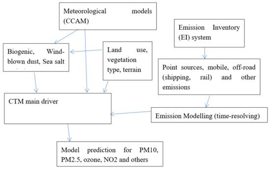
Figure 1.
Schematic structure of the emission and chemical transport model (CTM) modelling system.
- -
- It does not require boundary condition data as it is a global model that can be stretched to higher resolution at one particular region.
- -
- It can use CMIP5 climate projection data as host model data and does the climate projection based on the corresponding emission scenarios of the host model.
In this study, the CTM domain configuration consists of 4 nested grids, as shown in Figure 2, comprising the outermost Australia domain (75 × 65 grid cells) at 80 km × 80 km resolution, NSW (60 × 60 grid cells) at 27 km × 27 km, the Greater Metropolitan Region or GMR (60 × 60 grid cells) at 9 km × 9 km resolution and the innermost domain covering the Sydney region (60 × 60 grid cells) at 3 km × 3 km resolution.
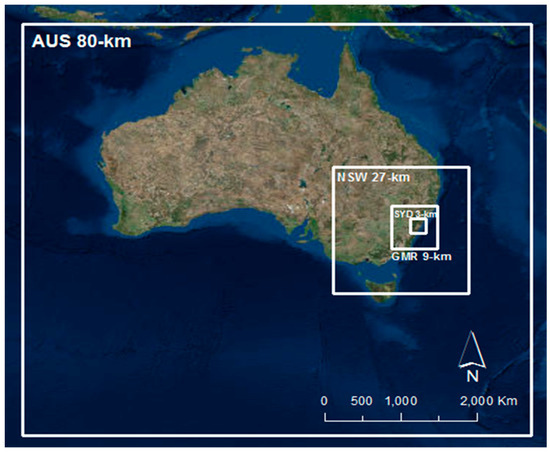
Figure 2.
The 4 nested domains for the CCAM-CTM (Cubic Conformal Atmospheric model-Chemical Transport model) simulation: Australia, NSW, GMR (Greater Metropolitan Region) and Sydney domains.
Further details of the domain setting, the model configurations as well as model validation as compared to observations can be found in [18] of this issue of Atmosphere.
2.2. Emission Modelling
The emission modelling embedded in the CCAM-CTM modelling system consists of natural and anthropogenic components. All natural emissions from the canopy, trees, grass pasture, soil, sea salt and dust were modelled and generated inline of CTM while the anthropogenic emissions were taken from the EPA NSW GMR Air Emissions Inventory for 2008 and prepared offline as input to the CTM.
The 2008 NSW GMR Air Emissions Inventory data, which is the latest inventory available to this study, was segregated into 17 major source groups: power generation from coal, power generation from gas, residential wood heaters, on-road vehicle petrol exhaust, diesel exhaust, other (e.g. LPG) exhaust, petrol evaporation, non-exhaust (e.g., brake) particulate matter, shipping and commercial boats, industrial vehicles and equipment, aircraft (flight and ground operations), locomotives, commercial non-road equipment, other commercial-domestic areas and industrial area fugitive sources, biogenic sources, and non-biogenic natural sources. Figure 3, as an example, shows the anthropogenic area source NO weekend emission for October 2008 and locations of power stations in the GMR. The source-dependent fraction for major source groups used in emission modelling is referenced in Appendix A of [18] in this issue of Atmosphere.
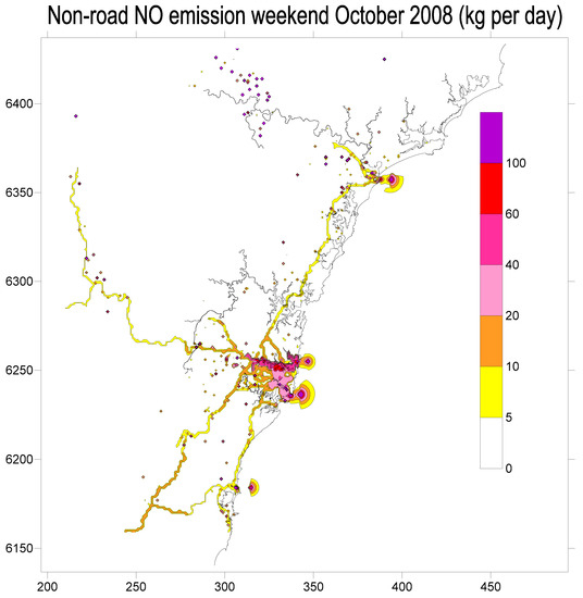
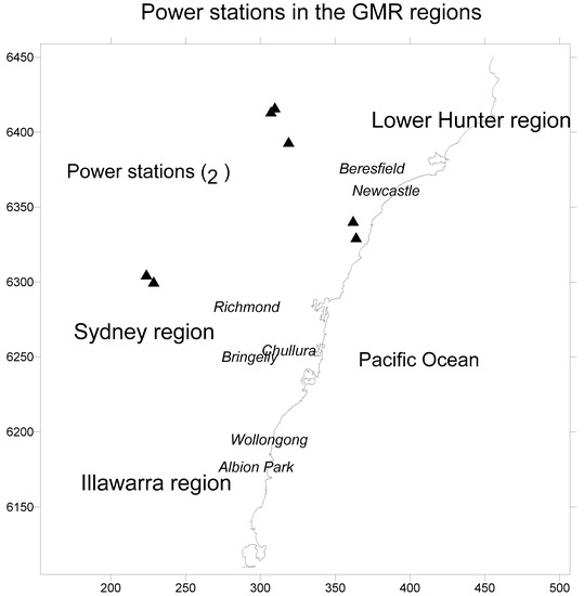
Figure 3.
Non-road area source NO weekend emission (above) for October 2008 (unit in kg/day) and locations of power stations in the GMR (bottom).
The emission of NOx and various species of VOC from area sources and power station point sources in the GMR for a typical summer month (January 2008 weekday) is shown in Table 1. These areas sources are commercial-domestic, locomotives, shipping, non-road commercial vehicles, industrial vehicles, passenger and light-duty petrol vehicles (VPX), passenger and light-duty diesel vehicles (VDX), all evaporative vehicle emission (VPV) and other vehicle exhaust (VLX).

Table 1.
Emission of NOx and VOC species from various area sources in the GMR for weekdays in January 2008.
The biogenic emission was modelled and generated inline in CTM. For ozone, the main biogenic contribution (VOC, NOx and NH3) is from vegetation and soil. The biogenic VOC is the sum of these species, isoprene, monoterpene, ethanol, methanol, aldehyde and acetone.
The biogenic emission consists of emission from forest canopies, pasture and grass and soil. The canopy model divides the canopy into an arbitrary number of vertical layers (typically 10 layers are used). Biogenic emissions from a forest canopy can be estimated from a prescription of the leaf area index, LAI (m2 m−2), the canopy height hc (m), the leaf biomass Bm (g m−2), and a plant genera-specific leaf level VOC emission rate Q (µg-C g−1 h−1) for the desired chemical species. The LAI used in CTM is based on Lu et al.’s [19] scheme which consists of LAI for trees and grass derived from an Advanced Very High-Resolution radiometer (AVHRR) normalized difference vegetation index (NDVI) data from between 1981 and 1994.
The biogenic NOx emission model from soil is based on the temperature-dependent Equation (1) [20].
where Qnox is the NOx emission rate at 30 °C and T is the soil temperature (°C).
Q = Qnox exp[0.71(T − 30)]
Ammonia (NH3) emission is based on Battye and Barrows’ scheme [21]. This approach uses annual average emission factors prescribed for four natural landscapes (forest, scrubland, pastureland, urban).
As shown in Figure 4, biogenic VOC emission occurs mostly in the west of Sydney and the Blue Mountain area, the National Park areas in the north, the lower Hunter region and inland of the Illawarra escarpment. In general, isoprene and monoterpene have similar spatial patterns as VOC distribution and reflect the Leaf Area Index (LAI) distribution in the modelling domain [12].
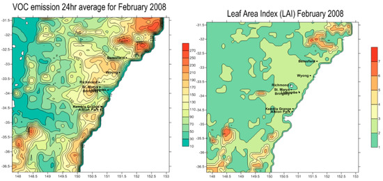
Figure 4.
VOC monthly 24-hourly average emission (kg/hour) (left) and Leaf Area Index (LAI) (right) for February 2008.
2.3. Emission Scenarios
The 2008 NSW GMR Air Emissions Inventory data was segregated into 16 major source groups, then re-grouped in to 8 categories, which are similar to those used by Karagulian, Belis et al. [22], to match the six identified categories using the component profile of the European Guide on Air Pollution Source Apportionment with Receptor Models for particles [23]. The emissions scenarios used in this study are: (1) All sources; (2) All anthropogenic—with emissions from all anthropogenic sources; (3) All natural—with emissions from all natural sources; (4) Power stations: emissions from coal and gas power generations; (5) On-road motor vehicles: emissions from petrol exhaust, diesel exhaust, other exhaust, petrol evaporative and non-exhaust particulate matter; (6) Non-road diesel and marine: with emissions from shipping and commercial boats, industrial vehicles and equipment, aircraft, locomotives, commercial non-road equipment; (7) Industry: with emissions from all point source except power generations from coal and gas; and (8) Commercial-domestic: with emissions from commercial and domestic-commercial area source excluding solid fuel burning (wood heaters). Wood heater emission is treated as a separate source category and in this study, which focused on summer ozone, there is no wood heating emission in the GMR.
2.4. The Integrated Empirical Rate (IER) Model
To determine the ozone production sensitivity to NOx and VOC, the IER model was used in this study. Central to the IER model is the concept of smog produced (SP). Photochemical smog is quantified in terms of NO oxidation which defines SP as the quantity of NO consumed by photochemical processes plus the quantity of O3 produced.
where and denote the NO and O3 concentrations that would exist in the absence of atmospheric chemical reactions occurring after time t = 0 and [NO]t and [O3]t are the NO and O3 concentrations existing at time t. denotes the concentration of smog produced by chemical reactions occurring during time t = 0 to time t = t.
When there is no more NO2 to be photolysed, and no more NO to react with reactive organic compounds to produce NO2 and nitrogen products (such as peroxyacetyl nitrate (PAN) species), ozone production is stopped. This condition in the photochemical process is called the NOx-limited regime. The ratio of the current concentration of SP to the concentration that would be present if the NOx-limited regime existed is defined as the parameter “Extent” of smog production (E). The extent value is indicative of how far toward attaining the NOx-limited regime the photochemical reactions have progressed. When E = 1, smog production is in the NOx-limited regime and the NO2 concentration approaches zero. When E < 1, smog production is in the light-limited (or VOC-limited) regime.
Previous studies have shown that high ozone levels in the west, north west and south west of Sydney are mostly in the regime of NOx-limited while central east Sydney is mostly light-limited (VOC-limited) [24]. For sensitivity analysis, it is expected that in the NOx-limited region, sensitivity of ozone to NOx emission change (say per-ton) is positive while it is negative in the VOC-limited region.
2.5. Source Attribution to Ozone Formation in Different Sub-Regions
Our study delineates the Greater Sydney Region into different sub-regions using the IER method and principal component analysis (PCA) statistical method. Source contribution to ozone formation was then determined in each of these sub-regions.
Using the 2008 summer (November 2007–March 2008) observed hourly monitoring data (NO, NO2, ozone and temperature) in the IER method, the extent of photochemical smog production in various Sydney sites was determined and then classified using a clustering statistical method. At a low level of pollutant concentrations, near background levels, with little or no photochemical reaction, the extent can be equal to 1. For this reason, to better classify the degree of photochemical reaction, the ozone level or the SP (smog produced) concentration has to be taken into account in addition to the extent variable.
Therefore, it is more informative to categorise the smog potential using both the extent value and the ozone concentration as:
- -
- Category A: extent > 0.8 and ozone conc. > 7 pphm
- -
- Category B: 0.5 < extent < 0.8 and 5 pphm < ozone conc. < 7 pphm
- -
- Category C: 0.5 < extent < 0.8 and 3 pphm < ozone conc. < 5 pphm
- -
- Category D: extent > 0.9 and ozone conc. < 3 pphm
Category A represents a very high ozone episode, Category B is a high ozone episode, Category C is a medium smog potential and Category D represents background or no smog production.
Using similar techniques as those of Yu and Chang [25], the principal component analysis (PCA) via correlation matrix on the 2007/2008 (1 November 2007 to 31 March 2008) summer ozone data was then used to delineate the regions in the Sydney area. The purpose of the PCA analysis is to transform the correlation coefficients between sites into component scores for each site based on the orthogonal principal components, in which the first component accounts for most of the variance and the second principal component the second most variance and so on. In this way, sites for which ozone are strongly related have similar component scores. Grouping the sites using a spatial contour plot of component scores identifies sites with similar ozone characteristics.
3. Results
3.1. Regional Delineation Using Integrated Empirical Rate (IER) Model and Principal Component Analysis (PCA)
The delineation of sub-regions in the GMR region based on their similar ozone formation patterns was performed using the clustering method and PCA method. These methods produced similar results. We present here the PCA results with component scores, which show that there are 3 principle components explaining most of the variances. The eigenvalues of the correlation matrix and the corresponding principal component scores for each site were derived. The contour plot of component scores for each component was used to delineate the regions.
The main sub-regions are western Sydney (North West, West, South West) and the coastal region consisting of astern Sydney, Lower Hunter and the Illawarra as shown in Figure 5a. The patterns of sub-regional delineation were similar to those from summer 1997/1998 [26,27] as depicted in Figure 5b. This means that over these 20 years, the spatial pattern of ozone formation did not show much change.
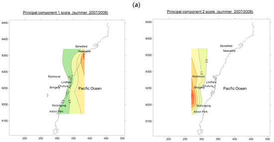
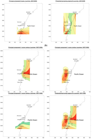
Figure 5.
Contour plots of the first 3 principal component scores depicting the regional delineation based on similarity of ozone formation pattern in (a) 2007/2008 and in (b) 1997/1998. The last plot in each graph is the combined plots of the 3 component score contours.
From the PCA analysis showing the spatial pattern of ozone formation, the Lower Hunter and Illawarra can be considered as separate from Sydney and the Sydney western region is separate from eastern and central Sydney. The western Sydney region is characterised as having a high frequency of smog events (NOx-limited or extent of smog production higher than 0.8). This is shown in Table 2, which shows the number of observed hourly data that are classified in each of the 4 smog potential categories for January 2008. Sites near the coast such as Randwick and Rozelle are in VOC-limited area with low smog events (zero number of observed hourly data in Category A and Category B).
Table 2.
Number of observed hourly data that are classified into each smog potential categories at different sites in the GMR for January 2008.
The Sydney western region is also sub-divided into 3 sub-regions, North West Sydney, West Sydney and South West Sydney. The North West is also influenced by sources in the Lower Hunter and the South West is related to some extent to the Illawarra region, as shown by the PCA analysis. The results confirmed previous studies [24,26,27], which have shown that the GMR region can be divided into sub-regions (north west, south west, west and central east) based on the ozone smog characteristics formed from the influence of meteorology and emission patterns in the GMR.
The GMR region was therefore divided into 6 sub-regions for this ozone source contribution study: Sydney North West, Sydney South West, Sydney West, Central and East Sydney, the Illawarra in the south and the Lower Hunter region in the north.
3.2. Source Contribution to Ozone over the Whole GMR
The CCAM-CTM predicted daily maximum 1-h and 4-h ozone concentrations in the GMR domain (9 km × 9 km) for the entire calendar year of 2008 under various emission scenarios are extracted at grid points nearest to the location of the 18 NSW Office of Environment and Heritage (OEH) air quality monitoring stations. Results from maximum 1-h and 4-h ozone analysis are very similar, therefore only results for 1-h predicted maximum ozone are presented.
Table 3 and Figure 6 shows the average source contributions to daily maximum 1-h ozone over the whole GMR. Apparently, natural sources are more significant in contributing to ozone concentration than all anthropogenic sources. During summer months (December, January and February), commercial and domestic, power stations and on-road motor vehicle sources contribute most to ozone formation in that order. During winter months (June, July and August), most of the anthropogenic sources contribute negatively to ozone formation (i.e., the presence of these sources decreases the level of ozone). Of the anthropogenic sources beside commercial-domestic sources, power stations contribute more to ozone formation within the whole GMR than that from on-road motor vehicles, industrial and non-diesel and marine sources in this order.
Table 3.
Monthly average of daily maximum 1-h predicted ozone concentration (ppb) in the GMR for different months in 2008 under various emission scenarios.
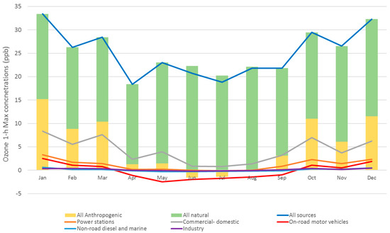
Figure 6.
Contribution of all anthropogenic and natural emissions (bar graph) and different anthropogenic sources (line graph) to the monthly average of daily maximum 1-h ozone concentration in 2008 in the GMR.
The monthly average of daily maximum 1-h ozone concentration for January 2008 for the 4 emission scenarios: base case, commercial-domestic sources off, power stations sources off and on-road mobile sources off is shown in Figure 7. The spatial pattern in daily maximum 1-h ozone from various source contribution is not uniform across the GMR as expected. The spatial pattern of maximum 1-h ozone shows that the relative importance of source contribution is different for different sub-regions.
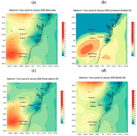
Figure 7.
Monthly average of daily maximum 1-h ozone concentration for January 2008 in (a) base case, (b) commercial-domestic sources off, (c) power stations sources off and (d) on-road mobile sources off emission scenarios.
3.3. Source Contribution to Ozone Concentrations over Sub-Regions within GMR
The daily maximum 1-h and 4-h predicted ozone concentrations under various emission scenarios are further analysed in this section to investigate the source contributions to ozone formation in each of the sub-regions across the GMR for 2008. As shown above from the PCA analysis, the different sub-regions have different smog characteristics as represented by the extent of smog production or NOx/VOC relationship with ozone level production. The 6 regions of the GMR are Sydney Northwest (Richmond and Vineyard), Sydney West (Bringelly, Prospect and St Marys), Sydney South West (Bargo, Liverpool and Oakdale), Sydney East (Chullora, Earlwood, Randwick and Rozelle), Illawarra (Albion Park, Kembla Grange and Wollongong) and Lower Hunter or Newcastle (Newcastle) regions. As for the whole GMR region analysis, only results for 1-h predicted ozone are presented here since the 4-h ones are very similar.
3.3.1. Sydney North West Region
This region is characterised as mostly NOx-limited during the ozone season (summer). Table 4 and Figure 8 show that of the anthropogenic sources, commercial-domestic sources (except wood heaters) contribute most to the 1-h ozone max, especially in the summer months. Power stations and motor vehicles are next in importance in contributing to ozone in the North West. Interestingly, during cold winter months, on-road motor vehicles have a negative contribution to maximum 1-h ozone in the North West of Sydney (i.e., increase in motor vehicle emission actually decreases the maximum ozone level in that region). This is due to the fact that photochemical ozone production never or rarely reaches NOx-limited during daytime, that is, mostly light-limited (or VOC-limited) regimes exist in the basin.
Table 4.
Monthly average of daily maximum 1-h ozone concentration (ppb) in the Sydney northwest region for different months in 2008 under various emission scenarios.
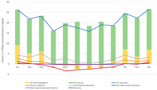
Figure 8.
Contribution of all anthropogenic and natural emissions (bar graph) and different anthropogenic sources (line graph) to the monthly average of daily maximum 1-h ozone concentration in 2008 in the Sydney northwest region.
To illustrate the change in ozone level in detail, Figure 9 shows the difference in predicted 1-h ozone (ppb) at Richmond for January 2008 between the base case and for scenarios when no biogenic emissions are present and when there is no emission from power stations. Biogenic emission significantly increases the ozone level and is the most important source contribution to the ozone maximum. Power station emission from the neighbouring region in the Lower Hunter also strongly influences the 1-h maximum ozone level in Sydney northwest, as is also shown in Figure 9. Note that, at night the ozone level is higher than the base case when coal-gas power station emissions are off as there is less NOx emission to scavenge the ozone.
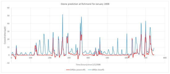
Figure 9.
Time series of difference in predicted 1-h ozone (ppb) at Richmond for January 2008 between the base case and biogenic emissions off (blue) and between the base case and power stations emissions off (red).
To summarise the whole distribution of predicted ozone with minimum, maximum, and median values, Figure 10 shows the box plots of the ozone prediction for January 2008 under different emission scenarios.
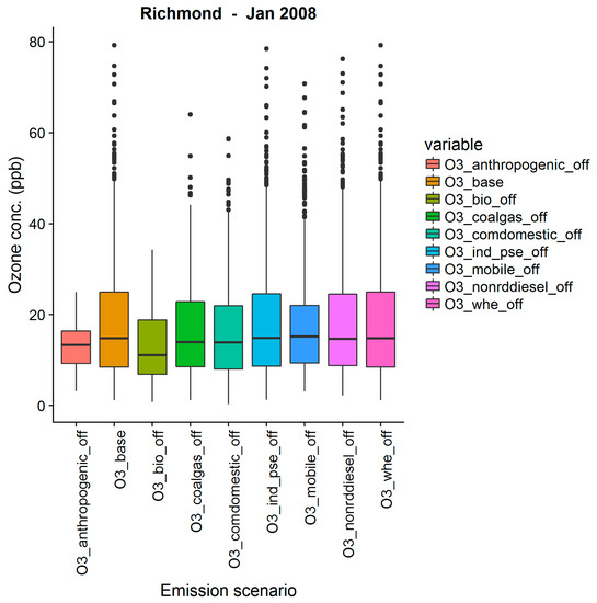
Figure 10.
Box plot for 1-h ozone concentration (ppb) in January 2008 under different emission scenarios at Richmond.
3.3.2. Sydney West, Sydney South West, Sydney East Regions
In the Sydney West region, the on-road motor vehicle emission has slightly more contribution to ozone 1-h max than that from power stations in the summer months. However, during cooler months in autumn and winter, motor vehicles have a negative contribution to daily maximum 1-h ozone levels.
Appendix A shows the tables and graphs summarising the effect of each source to the ozone formation in each of the regions. As shown in Figure A6 (Appendix A) of the ozone concentration at Chullora for January 2008, even though the monthly maximum is reduced when the mobile source is turned off, the median ozone increased slightly. This is because the night time ozone increases when there is less NOx emission to scavenge the ozone. The ozone level also increases during the day time, when ozone level is low and in a VOC-limited photochemical process, if NOx emission is decreased. This can be seen in the time series of difference in predicted ozone levels at Chullora for January 2008 under the base case and no motor vehicle emission scenario, as shown in Figure 11. Maximum ozone is reduced for days where the ozone is high, but for days when ozone is low and at night, the ozone level is higher when motor vehicle emission is turned off. The time series shows that for most of the time during January 2008, Chullora is in a VOC-limited regime. Also shown in Figure 11, is the time series of difference in predicted ozone under the base case and when no power station emission is present. Higher levels of local NOx due to emission from motor vehicles compared to that received downwind from power stations has a more dramatic effect on ozone level at Chullora.
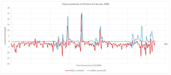
Figure 11.
Time series of difference in predicted 1-h ozone (ppb) at Chullora for January 2008 between the base case and motor vehicle emissions off (red) and between the base case and power station emissions off (blue).
3.3.3. Illawarra and Lower Hunter Regions
The results for the Illawarra and Lower Hunter regions are described in Appendix Table A4 and Table A5.
Table 5 summarises the order of importance in source contribution to 1-h ozone maximum in each of the 6 sub-regions of the GMR Sydney region.
Table 5.
Ranked order of contribution from anthropogenic sources to maximum 1-h ozone (warm months). For Central and East Sydney, motor vehicle or industry emission decreases the maximum 1-h ozone (negative contribution) and is denoted by x in the table.
4. Discussion
Air quality models have been used recently by various authors to study the source contribution to air pollution concentration at a receptor. The main models that are currently used are the source-oriented CMAQ model and the CAMx model with OSAT. The main advantage of these models is that they treat emitted species from different sources separately, and hence, can identify source contributions to ozone in a single model run rather than the multiple runs required by chemical transport models (CTM), using brute force or zero-out method as used in this study [11].
Caiazzo et al. [28], in their study to quantify the impact of major sectors on air pollution and early death in the whole US in 2005 using WRF/CMAQ model, estimated that ~10,000 (90% CI: −1000 to 21,000) premature deaths per year were due to changes in maximum ozone concentrations. The largest contributor to early deaths due to increases in maximum ozone is road transportation with ~5000 (90% CI: −900 to 11,000) followed by power generation with ~2000 (90% CI: −300 to 4000) early deaths per year.
Our study on source contribution to ozone formation in the Greater Metropolitan Region (GMR) of Sydney in 2008 identified biogenic sources (mainly vegetation via isoprene and monoterpene emission) as the major contributor to ozone formation in all regions of the GMR. This result confirms the previous study of Duc et al. [8] on ozone source contribution in the Sydney Particle Study (SPS) in January 2011. Similarly, Ying and Krishnan [29] in their study of source contribution of VOC in southeast Texas based on simulation using the CMAQ model, found that for maximum 8-h ozone occurrences from 16 August to 7 September 2000, the median of relative contributions from biogenic sources was approximately 60% compared to 40% from anthropogenic ones. As biogenic emission is a major contribution to ozone formation, it is important for the model to account for it as accurately as possible. Emmerson et al. [30] found that the Australian Biogenic Canopy and Grass Emission Model (ABCGEM), as implemented in the CCAM-CTM model used in this study, accounts for biogenic VOC emission (especially monoterpenes) from Australian eucalyptus vegetation better than the model of Emissions of Gases and Aerosols from Nature (MEGAN) when these modelled emissions are compared with observations.
Among the anthropogenic sources, commercial and domestic sources are the main contributors to ozone concentration in all regions. Power station or motor vehicle sources, depending on the region, are the next main contributors to ozone formation. However, in the cooler months, these sources (power stations and motor vehicles) decrease the level of ozone. From Table 1, commercial and domestic sources (except wood heaters) have much higher emission of most VOC species than other sources, even though they emit less NOx than other mobile sources. For this reason, it is not surprising that commercial and domestic sources contribute most to the ozone formation in all the metropolitan regions.
As it is not possible or practical to control biogenic emission sources, the implication of this study is that to control the level of ozone in the GMR, commercial and domestic sources should be the focus for policy makers to manage the ozone level in the GMR. As shown in Figure 7, when commercial domestic sources are turned off, a reduction in ozone is attained in all regions in the GMR.
A reduction in power station emission will significantly improve the ozone concentration in the North West of Sydney, but less so in other regions of the GMR. Gégo et al. [31] in their study of the effects of change in nitrogen oxide emissions from the electric power sector on ozone levels in the eastern U.S, using the CMAQ model for 2002, have shown that ozone concentrations would have been much higher in much of the eastern United States if NOx emission controls had not been implemented by the power sector, and exceptions occurred in the immediate vicinity of major point sources where increased NO titration tends to lower ozone levels.
Motor vehicles are less a problem compared to commercial-domestic and power station sources except for the South West of Sydney. However, the South West of Sydney has more smog episodes than other regions in the GMR, therefore, to reduce the high frequency of ozone events, control of motor vehicle emission should be given more priority than control of emission from power station sources. As shown in Figure 7, compared to other regions, a significant reduction of ozone in the South West is achieved when on-road mobile sources were turned off. This region is downwind from the urban area of Sydney, where the largest emission source of NOx and VOC precursors is motor vehicles, and hence, causes elevated ozone downwind in the South West of Sydney. Various studies have shown that areas downwind from the upwind emission of precursors experience high ozone [32,33].
Reduction in motor vehicle emission benefits the South West of Sydney but instead increases the daily average ozone level in the east of the Sydney region where most motor vehicle emission occurs even though this does not affect the maximum ozone level in this region.
Similar to our study, the source contribution to ozone in the Pearl River Delta (PRD) region of China was studied by Li et al. [11] who divided the whole modelling domain including the PRD and Hong Kong regions, south China region and the whole of China into 12 source areas and 7 source categories which include anthropogenic sources outside PRD, biogenic, shipping, point sources, areas sources such as domestic and commercial and mobile sources in PRD, and in Hong Kong. Their results showed that under mean ozone conditions, super-regional (outside regional and PRD areas) contribution is dominant but, for high ozone episodes, elevated regional and local sources are still the main causative factors. Among all the sources, the mobile source is the category that contributes most to ozone in the PRD region. They also showed that ozone in the upwind area of the Pearl River Delta is mostly affected by super-regional sources and local sources while the downwind area has higher ozone and is affected by regional sources in its upwind area besides the super-regional and local source contribution. This is not surprising as the mobile source is the dominant local source emission in the PRD area, and hence, downwind areas are mostly affected by this source in the ozone formation.
It should be noted that our results on the source contribution to ozone is only applied to the base 2008 emission inventory data. If this “base state” of emission is changed so that there is a different composition of VOC and NOx emissions (such as the 2013 or 2018 emission inventories), then the source contribution results could be different because the relation of ozone formation with VOC and NOx precursors emissions at various regions in the GMR is nonlinear and complex.
As ozone response to emitting sources of VOC and NOx is nonlinear, the contribution of each source to maximum ozone is dependent on the “base state” consisting of all other emitting sources in the region. Therefore, uncertainty in the emission inventory of these sources also affects the contribution of ozone attributed to this source. Cohan et al. [1] has shown that underestimates of NOx emission rates lead to underprediction of the total source contribution but overprediction of per-ton sensitivity.
Fujita et al. [34] in their study of source contributions of ozone precursors in California’s South Coast Air Basin to ozone weekday and weekend variation showed that reduced NOx emission of weekend emission from motor vehicle caused higher level of ozone than during the weekday due to the higher ratio of NMHC (non-methane hydrocarbon) to NOx in this VOC-limited basin. Conversely, Collet et al. [35] in their study of ozone source attribution and sensitivity analysis across the U.S showed that, in most of the locations, reduction in NOx emission is more effective than reduction in VOC emission in reducing ozone levels.
It is therefore important to determine and understand which region in the GMR is NOx-limited or VOC-limited. The observation-based IER method which uses monitoring station data has proved to be useful in delineation of the different regions of photochemical smog profiles, within the GMR where monitoring stations are located. Based on the results from the IER method, the results of source contribution to maximum ozone in the GMR using an air quality model for different emission scenarios can be understood and explained adequately from an emission point of view, and therefore, can facilitate policy implementation.
As for policy implementation in reducing ozone, it should be pointed out that even though Sydney ozone trend in the past decade has decreased, the background ozone trend is actually increasing [36], which is part of a world-wide trend of increasing background ozone levels. This will make the further reduction of ozone in the future much more difficult, as shown and discussed by Parrish et al. [37] in their study of background ozone contribution to the California air basins.
5. Conclusions
This study provides a detailed source contribution to ozone formation in different regions of the Greater Metropolitan Regions of Sydney. The importance of each source in these regions is depending on the ozone formation potential of each of these regions, and whether they are in NOx-limited or VOC-limited photochemical regimes in the ozone season. Extensive monitoring data available from the OEH monitoring network and many previous studies using observation-based methods have provided an understanding of the ozone formation potential in various sub-regions of the GMR.
Biogenic emission is the major contributor to ozone formation in all regions of the GMR due to their large emission of VOC. Of anthropogenic emissions, commercial and domestic sources are the main contributors to ozone concentration in all regions. These commercial and domestic sources (except wood heaters) have much higher emission of most VOC species but less NOx than other sources, such as mobile sources, and hence contribute more to ozone formation in all the metropolitan regions compared to other sources. The commercial and domestic sources should be the focus for policy makers to manage the ozone level in the GMR.
Furthermore, based on the results of this study, the following policy-relevant suggestions are proposed to regulate the ozone level in particular Sydney regions:
- -
- In the North West of Sydney, power station emission control will improve the ozone concentration there as well as in the Lower Hunter and the Illawarra regions.
- -
- In the South West of Sydney, which has more smog episodes than other regions in the GMR, control of motor vehicle emissions should be given priority to reduce the high frequency of ozone events in the Sydney basin.
Our next study in relation to source contribution to ozone formation will focus on the health impact of each emission source on various health endpoints from their contribution to poor air quality (e.g., ozone and PM2.5) in the GMR.
Author Contributions
Conceptualization, H.N.D.; methodology, H.N.D., L.T.-T.C.; software, H.N.D., T.T., D.S.; validation, L.T.-T.C., T.T. and D.S.; formal analysis, H.N.D.; investigation, H.N.D., L.T.-T.C.; resources, H.N.D., D.S., Y.S.; data curation, H.N.D., L.T.-T.C., T.T., D.S.; writing—original draft preparation, H.N.D.; writing—review and editing, H.N.D., L.T.-T.C.; visualization, H.N.D., L.T.-T.C.; supervision, H.N.D.; project administration, Y.S.; funding acquisition, Clare Murphy.
Funding
This research received no external funding except support from Clean Air and Urban Landscapes (CAUL) Research Hub for the retreat conference.
Acknowledgments
Open access funding for this work was provided from the Office of Environment & Heritage, New South Wales (OEH, NSW).
Conflicts of Interest
The authors declare no conflict of interest.
Appendix A
Appendix A.1. Sydney West Region
Table A1.
Monthly average of daily maximum 1-h predicted ozone concentration (ppb) in the Sydney west region for different months in 2008 under various emission scenarios.
Table A1.
Monthly average of daily maximum 1-h predicted ozone concentration (ppb) in the Sydney west region for different months in 2008 under various emission scenarios.
| Month | All Sources | Power Stations | Commercial-Domestic | On-Road Motor Vehicles | Non-Road Diesel and Marine | Industry | All Anthropogenic | All Natural |
|---|---|---|---|---|---|---|---|---|
| January | 38.53 | 4.02 | 10.23 | 5.24 | 0.52 | 0.28 | 20.29 | 18.23 |
| February | 29.33 | 2.52 | 6.83 | 1.72 | 0.11 | 0.64 | 11.82 | 17.51 |
| March | 31.89 | 1.24 | 10.57 | 1.66 | −0.07 | 0.32 | 13.72 | 18.17 |
| April | 18.61 | 0.09 | 2.95 | −1.44 | −0.08 | 0.09 | 1.63 | 16.97 |
| May | 23.6 | 0.36 | 4.8 | −2.94 | −0.16 | 0.02 | 2.19 | 21.41 |
| June | 20.68 | 0.13 | 0.88 | −1.97 | −0.18 | −0.14 | −1.26 | 21.94 |
| July | 18.99 | −0.04 | 0.86 | −1.42 | −0.09 | −0.04 | −0.72 | 19.71 |
| August | 22.27 | 0.01 | 1.58 | −1.25 | −0.09 | −0.01 | 0.29 | 21.98 |
| September | 23.02 | 1.53 | 3.47 | −0.84 | −0.01 | 0.19 | 4.38 | 18.63 |
| October | 32.28 | 2.39 | 8.24 | 2.5 | 0.24 | 0.48 | 13.87 | 18.41 |
| November | 28.36 | 1.69 | 4.8 | 0.96 | 0.15 | 0.19 | 7.79 | 20.57 |
| December | 34.12 | 2.33 | 6.62 | 3.24 | 0.36 | 0.47 | 13.03 | 21.09 |
| Average | 26.84 | 1.35 | 5.17 | 0.46 | 0.06 | 0.21 | 7.27 | 19.56 |
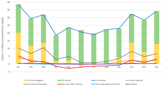
Figure A1.
Contribution of all anthropogenic and natural emissions (bar graph) and different anthropogenic sources (line graph) to the monthly average of daily maximum 1-h ozone concentration in 2008 in the Sydney west region.
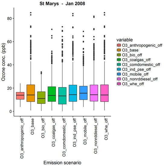
Figure A2.
Box plot for 1-h ozone concentration (ppb) in January 2008 under different emission scenarios at St Marys.
Appendix A.2. Sydney South West Region
In the Sydney south west region, which is mostly NOx-limited during the ozone season and is downwind from the Sydney central east region, the on-road motor vehicle emission has a greater contribution to daily maximum 1-h ozone than that from power stations in the summer months. Next is industry and then non-diesel and shipping sources. in that order as the ranked contribution to ozone concentration.
Table A2.
Monthly average of daily maximum 1-h predicted ozone concentration (ppb) in the Sydney south west region for different months in 2008 under various emission scenarios.
Table A2.
Monthly average of daily maximum 1-h predicted ozone concentration (ppb) in the Sydney south west region for different months in 2008 under various emission scenarios.
| Month | All Sources | Power Stations | Commercial-Domestic | On-Road Motor Vehicles | Non-Road Diesel and Marine | Industry | All Anthropogenic | All Natural |
|---|---|---|---|---|---|---|---|---|
| January | 38.05 | 3.12 | 8.76 | 5.41 | 0.79 | 1.31 | 19.4 | 18.65 |
| February | 27.07 | 1.54 | 4.79 | 1.78 | 0.4 | 0.95 | 9.46 | 17.61 |
| March | 31.66 | 1.75 | 8.17 | 1.96 | 0.35 | 1.11 | 13.35 | 18.32 |
| April | 19.76 | 0.23 | 2.01 | −0.11 | 0.11 | 0.26 | 2.52 | 17.24 |
| May | 24.62 | 0.54 | 2.91 | −1.1 | 0.07 | 0.27 | 2.76 | 21.86 |
| June | 21.71 | 0.11 | 0.63 | −1.29 | −0.06 | −0.05 | −0.64 | 22.35 |
| July | 19.7 | −0.01 | 0.62 | −1.26 | −0.07 | −0.09 | −0.8 | 20.5 |
| August | 22.37 | 0.05 | 0.85 | −0.81 | −0.02 | 0.05 | 0.16 | 22.21 |
| September | 21.97 | 0.89 | 2.25 | −0.51 | 0.05 | 0.21 | 2.92 | 19.06 |
| October | 29.87 | 1.81 | 5.66 | 2.22 | 0.46 | 0.83 | 11 | 18.86 |
| November | 27.91 | 1.18 | 4.29 | 1.1 | 0.21 | 0.5 | 7.28 | 20.63 |
| December | 31.4 | 1.62 | 4.83 | 2.26 | 0.49 | 0.74 | 9.95 | 21.45 |
| Average | 26.37 | 1.07 | 3.83 | 0.81 | 0.23 | 0.51 | 6.47 | 19.91 |
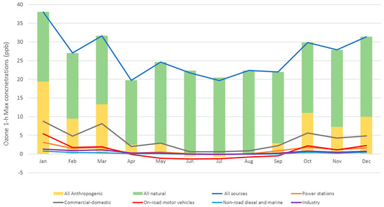
Figure A3.
Contribution of all anthropogenic and natural emissions (bar graph) and different anthropogenic sources (line graph) to the monthly average of daily maximum 1-h ozone concentration in 2008 in the Sydney South West region.
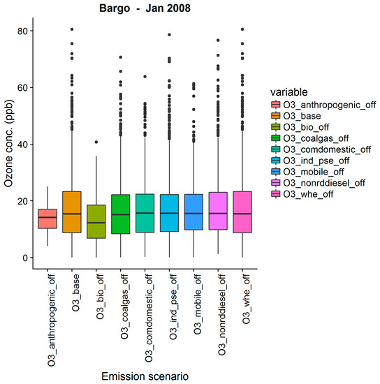
Figure A4.
Box plot for 1-h ozone concentration (ppb) in January 2008 under different emission scenarios at Bargo.
Appendix A.3. Sydney East Region
In the Sydney east region, the motor vehicle emission, on average for each month, contributes negatively to the 1-h maximum ozone concentration in all months of 2008 in this region (as represented by the 3 sites listed above). As this region is in a light-limited regime (or VOC-limited), an increase in NOx emission from motor vehicle sources will reduce the ozone level.
Table A3.
Monthly average of daily maximum 1-h predicted ozone concentration (ppb) in the Sydney east region for different months in 2008 under various emission scenarios.
Table A3.
Monthly average of daily maximum 1-h predicted ozone concentration (ppb) in the Sydney east region for different months in 2008 under various emission scenarios.
| Month | All Sources | Power Stations | Commercial-Domestic | On-Road Motor Vehicles | Non-Road Diesel and Marine | Industry | All Anthropogenic | All Natural |
|---|---|---|---|---|---|---|---|---|
| January | 27.91 | 2.29 | 8.63 | −0.88 | 0.09 | 0.16 | 10.29 | 17.61 |
| February | 23.5 | 1.41 | 6.07 | −0.82 | −0.3 | 0.17 | 6.53 | 16.97 |
| March | 22.79 | 0.93 | 6.59 | −1.96 | −0.37 | 0.12 | 5.32 | 17.47 |
| April | 15.82 | 0.09 | 1.98 | −2.37 | −0.46 | −0.1 | −0.84 | 16.66 |
| May | 18.94 | 0.05 | 4.05 | −5.08 | −0.88 | −0.17 | −1.9 | 20.85 |
| June | 17.77 | −0.01 | 0.82 | −3.67 | −0.77 | −0.26 | −3.88 | 21.65 |
| July | 15.79 | −0.11 | 0.81 | −3.46 | −0.68 | −0.18 | −3.6 | 19.39 |
| August | 19.39 | 0.03 | 1.43 | −3.02 | −0.51 | −0.13 | −2.16 | 21.55 |
| September | 19.32 | 0.29 | 3.91 | −2.39 | −0.62 | −0.02 | 1.2 | 18.12 |
| October | 26.23 | 2.04 | 8.14 | −1.61 | −0.32 | 0.12 | 8.39 | 17.85 |
| November | 23.79 | 1.11 | 3.38 | −0.85 | −0.09 | 0.13 | 3.68 | 20.11 |
| December | 30.73 | 2.26 | 8.31 | −0.37 | 0.17 | 0.34 | 10.71 | 20.01 |
| Average | 21.85 | 0.87 | 4.52 | −2.21 | −0.39 | 0.02 | 2.82 | 19.03 |
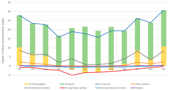
Figure A5.
Contribution of all anthropogenic and natural emissions (bar graph) and different anthropogenic sources (line graph) to the monthly average of daily maximum 1-h ozone concentration in 2008 in the Sydney east region.
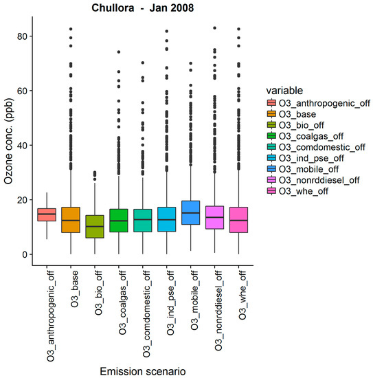
Figure A6.
Box plot for 1-h ozone concentration (ppb) in January 2008 under different emission scenarios at Chullora.
Appendix A.4. the Illawarra Region
In the Illawarra region, after commercial and domestic sources, power stations and motor vehicles are next in importance in contributing to ozone formation.
Table A4.
Monthly average of daily maximum 1-h predicted ozone concentration (ppb) in the Illawarra region for different months in 2008 under various emission scenarios.
Table A4.
Monthly average of daily maximum 1-h predicted ozone concentration (ppb) in the Illawarra region for different months in 2008 under various emission scenarios.
| Month | All Sources | Power Stations | Commercial-Domestic | On-road Motor vehicles | Non-Road Diesel and Marine | Industry | All Anthropogenic | All Natural |
|---|---|---|---|---|---|---|---|---|
| January | 33.99 | 4.02 | 8.99 | 2.48 | 0.48 | −0.1 | 15.86 | 18.13 |
| February | 27.45 | 2 | 5.87 | 1.82 | 0.14 | 0.21 | 10.05 | 17.41 |
| March | 29.34 | 1.75 | 8.02 | 1.4 | 0.08 | 0 | 11.25 | 18.1 |
| April | 18.36 | 0.19 | 2.44 | −1.05 | −0.1 | −0.12 | 1.37 | 16.99 |
| May | 23.35 | 0.43 | 3.84 | −2.09 | −0.2 | −0.25 | 1.82 | 21.53 |
| June | 20.78 | 0.05 | 0.82 | −1.9 | −0.22 | −0.21 | −1.45 | 22.23 |
| July | 19.04 | −0.02 | 0.72 | −1.59 | −0.14 | −0.11 | −1.12 | 20.16 |
| August | 22.22 | 0.12 | 1.21 | −1.2 | −0.07 | −0.04 | 0.06 | 22.16 |
| September | 21.85 | 1.22 | 2.96 | −0.92 | −0.08 | −0.01 | 3.2 | 18.65 |
| October | 29.7 | 2.69 | 6.94 | 1.28 | 0.23 | 0.18 | 11.35 | 18.35 |
| November | 26.68 | 1.76 | 3.65 | 0.62 | 0.22 | −0.11 | 6.14 | 20.54 |
| December | 32.17 | 2.39 | 5.95 | 2.23 | 0.52 | 0.25 | 11.33 | 20.84 |
| Average | 25.44 | 1.39 | 4.3 | 0.09 | 0.07 | −0.03 | 5.84 | 19.6 |
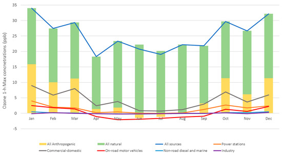
Figure A7.
Contribution of all anthropogenic and natural emissions (bar graph) and different anthropogenic sources (line graph) to the monthly average of daily maximum 1-h ozone concentration in 2008 in the Illawarra region.
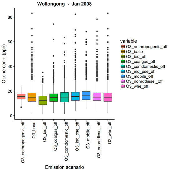
Figure A8.
Box plot for 1-h ozone concentration (ppb) in January 2008 under different emission scenarios at Wollongong.
Appendix A.5. The Lower Hunter (Newcastle) Region
In the Lower Hunter (Newcastle) region, power stations, non-road diesel and shipping sources are more important than motor vehicle and industrial sources.
Table A5.
Monthly average of daily maximum 1-h predicted ozone concentration (ppb) in the Newcastle region for different months in 2008 under various emission scenarios.
Table A5.
Monthly average of daily maximum 1-h predicted ozone concentration (ppb) in the Newcastle region for different months in 2008 under various emission scenarios.
| Month | All Sources | Power Stations | Commercial-Domestic | On-Road Motor Vehicles | Non-Road Diesel and Marine | Industry | All Anthropogenic | All Natural |
|---|---|---|---|---|---|---|---|---|
| January | 24.91 | 0.78 | 3.65 | 0.33 | 1.64 | 0.25 | 6.67 | 18.25 |
| February | 25.55 | 1.10 | 5.00 | 0.92 | 0.73 | 0.25 | 8.00 | 17.55 |
| March | 25.52 | 0.95 | 4.12 | 0.67 | 1.19 | 0.40 | 7.35 | 18.17 |
| April | 20.82 | −0.10 | 3.31 | −0.19 | −0.05 | −0.01 | 3.01 | 17.80 |
| May | 25.49 | −0.98 | 5.44 | −0.62 | −0.38 | −0.02 | 3.51 | 21.98 |
| June | 23.24 | −1.18 | 2.47 | −0.62 | −0.38 | −0.09 | 0.23 | 23.00 |
| July | 20.91 | −1.00 | 1.46 | −0.52 | −0.31 | −0.04 | −0.38 | 21.30 |
| August | 23.77 | −1.15 | 3.05 | −0.44 | −0.18 | 0.00 | 1.37 | 22.40 |
| September | 24.69 | 0.98 | 3.95 | 0.26 | 0.30 | 0.13 | 5.65 | 19.04 |
| October | 29.86 | 3.28 | 6.16 | 0.43 | 1.00 | 0.26 | 11.16 | 18.70 |
| November | 26.06 | 1.63 | 3.27 | 0.52 | 0.60 | 0.22 | 6.24 | 19.82 |
| December | 34.31 | 3.91 | 7.81 | 1.12 | 1.37 | 0.45 | 14.66 | 19.65 |
| Average | 25.45 | 0.69 | 4.15 | 0.15 | 0.46 | 0.15 | 5.63 | 19.82 |
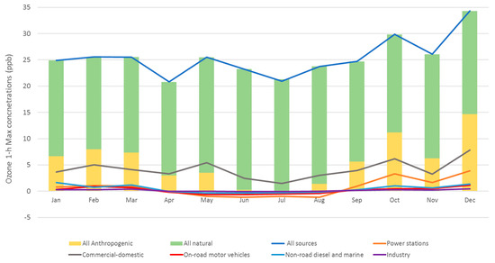
Figure A9.
Contribution of all anthropogenic and natural emissions (bar graph) and different anthropogenic sources (line graph) to the monthly average of daily maximum 1-h ozone concentration in 2008 in the Newcastle region.
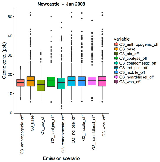
Figure A10.
Box plot for 1-h ozone concentration (ppb) in January 2008 under different emission scenarios at Newcastle.
References
- Cohan, D.; Hakami, A.; Hu, Y.; Russell, A.G. Nonlinear Response of Ozone to Emissions: Source Apportionment and Sensitivity Analysis. Environ. Sci. Technol. 2005, 39, 6739–6748. [Google Scholar] [CrossRef] [PubMed]
- Blanchard, C.; Stoeckenius, T. Ozone response to precursor controls: Comparison of data analysis methods with the predictions of photochemical air quality simulation models. Atmos. Environ. 2001, 35, 1203–1215. [Google Scholar] [CrossRef]
- Johnson, G. A simple model for predicting the ozone concentration of ambient air. In Proceedings of the Eight International Clean Air Conference, Melbourne, Australia, 7–11 May 1984; pp. 715–731. [Google Scholar]
- Blanchard, C. Ozone process insights from field experiments—Part III: Extent of reaction and ozone formation. Atmos. Environ. 2000, 34, 2035–2043. [Google Scholar] [CrossRef]
- Blanchard, C.; Fairley, D. Spatial mapping of VOC and NOx-limitation of ozone formation in central California. Atmos. Environ. 2001, 35, 3861–3873. [Google Scholar] [CrossRef]
- Dunker, A.; Yarwood, G.; Ortmann, J.; Wilson, G. The decoupled direct method for sensitivity analysis in a three-dimensional air quality model—Implementation, accuracy, and efficiency. Environ. Sci. Technol. 2002, 36, 2965–2976. [Google Scholar] [CrossRef] [PubMed]
- Buzcu, B.; Fraser, M. Source identification and apportionment of volatile organic compounds in Houston, TX. Atmos. Environ. 2006, 40, 2385–2400. [Google Scholar] [CrossRef]
- Ling, H.; Guo, H.; Cheng, H.R.; Yu, Y.F. Sources of ambient volatile organic compounds and their contributions to photochemical ozone formation at a site in the Pearl River Delta, southern China. Environ. Pollut. 2011, 159, 2310–2319. [Google Scholar] [CrossRef] [PubMed]
- Gaimoz, C.; Sauvage, S.; Gros, V. Volatile organic compounds sources in Paris in spring 2007. Part II: Source apportionment using positive matrix factorization. Environ. Chem. 2011, 8, 91–103. [Google Scholar] [CrossRef]
- Dunker, A.; Yarwood, G.; Ortmann, J.; Wilson, G. Comparison of source apportionment and source sensitivity of ozone in a three-dimensional air quality model. Environ. Sci. Technol. 2002, 36, 2953–2964. [Google Scholar] [CrossRef] [PubMed]
- Li, K.; Lau, A.; Fung, J.C.-H.; Zheng, J.Y.; Zhong, L.J.; Louie, P.K.K. Ozone source apportionment (OSAT) to differentiate local regional and super-regional source contributions in the Pearl River Delta region, China. J. Geophys. Res. 2012, 117, D15305. [Google Scholar] [CrossRef]
- Duc, H.; Trieu, T.; Metia, S. Source contribution to ozone and PM2.5 formation in the Greater Sydney Region during the Sydney Particle Study 2011. In Proceedings of the 23th International Clean Air & Environment Conference, Brisbane, Australia, 15–18 October 2017. [Google Scholar]
- Nguyen, V.; Soulhac, L.; Salizzoni, P. Source Apportionment and Data Assimilation in Urban Air Quality Modelling for NO2: The Lyon Case Study. Atmosphere 2018, 9, 8. [Google Scholar] [CrossRef]
- Wang, X.; Li, J.; Zhang, Y.; Xie, S.; Tang, X. Ozone source attribution during a severe photochemical smog episode in Beijing, China. Sci. China Ser. B Chem. 2009, 52, 1270–1280. [Google Scholar] [CrossRef]
- Zhang, H.; Li, J.; Ying, Q.; Yu, J.Z.; Wu, D.; Cheng, Y.; He, K.; Jiang, J. Source apportionment of PM2.5 nitrate and sulfate in China using a source-oriented chemical transport model. Atmos. Environ. 2012, 62, 228–242. [Google Scholar] [CrossRef]
- Duc, H.; Spencer, J.; Quigley, S.; Trieu, T. Source contribution to ozone formation in the Sydney airshed. In Proceedings of the 21th International Clean Air & Environment Conference, Sydney, Australia, 7–11 September 2013. [Google Scholar]
- Thatcher, M.; McGregor, J. Using a Scale-Selective Filter for Dynamical Downscaling with the Conformal Cubic Atmospheric Model. Mon. Weather Rev. 2009, 137, 1742–1752. [Google Scholar] [CrossRef]
- Chang, L.T.-C.; Duc, H.; Scorgie, Y.; Trieu, T.; Monk, K.; Jiang, N. Performance Evaluation of CCAM-CTM Regional Airshed Modelling for the New South Wales Greater Metropolitan Region. Atmosphere 2018. submitted. [Google Scholar]
- Lu, H.; Raupach, M.; McVicar, T.R.; Barrett, D.J. Decomposition of vegetation cover into woody and herbaceous components using AVHRR NDVI time series. Remote Sens. Environ. 2003, 86, 1–18. [Google Scholar] [CrossRef]
- Williams, E.; Guenther, A.; Fehsenfeld, F. An inventory of nitric oxide emissions from soils in the United States. J. Geophys. Res. 1992, 97, 7511–7519. [Google Scholar] [CrossRef]
- Battye, B.; Barrows, R. Review of Ammonia Emission Modeling Techniques for Natural Landscape and Fertilized Soils; Prepared for Thomas Pierce, US EPA. EC/R Incorporated: Chapel Hill, NC, USA, May 2004. Available online: https://www.researchgate.net/publication/267786537_Review_of_Ammonia_Emission_Modeling_Techniques_for_Natural_Landscapes_and_Fertilized_Soils (accessed on 7 September 2018).
- Karagulian, F.; Belis, C.; Francisco, C.; Prüss-Ustün, A.M.; Bonjour, S.; Adair-Rohani, H.; Amann, M. Contributions to cities’ ambient particulate matter (PM): A systematic review of local source contributions at global level. Atmos. Environ. 2015, 120, 475–483. [Google Scholar] [CrossRef]
- Belis, C.; Larsen, B.; Amato, F.; El Haddad, I.; Favez, O.; Harrison, R.; Hopke, P.; Nava, S.; Paatero, P.; Prevot, A.; et al. European Guide on Air Pollution Source Apportionment with Receptor Models; European Commission, Joint Research Centre, Institute for Environment and Sustainability, JRC-Reference Reports; Publications Office of the European Union: Luxembourg, 2014. [Google Scholar]
- Duc, H.; Azzi, M.; Quigley, S. Extent of photochemical smog reaction in the Sydney metropolitan areas. In Proceedings of the MODSIM 2003, International Congress on Modelling and Simulation, Townsville, Australia, 14–17 July 2003; pp. 76–81. [Google Scholar]
- Yu, T.; Chang, L. Delineation of air-quality basins utilizing multivariate statistical methods in Taiwan. Atmos. Environ. 2001, 35, 3155–3166. [Google Scholar] [CrossRef]
- Anh, V.; Azzi, M.; Duc, H.; Johnson, G. Classification of air quality monitoring stations in the Sydney basin. In Proceedings of the Asia-Pacific Conference on Sustainable Energy and Environmental Technology, Singapore, 19–21 June 1996; pp. 266–271. [Google Scholar]
- Duc, H.; Azzi, M.; Quigley, S. Extent analysis of historical photochemical smog events in the Sydney metropolitan areas. In Proceedings of the National Clean Air Conference, Newcastle, Australia, 23–27 November 2003. [Google Scholar] [CrossRef]
- Caiazzo, F.; Ashok, A.; Waitz, I.A.; Yim, S.H.L.; Barrett, S.R.H. Air pollution and early deaths in the United States. Part I: Quantifying the impact of major sectors in 2005. Atmos. Environ. 2013, 79, 198–208. [Google Scholar] [CrossRef]
- Ying, Q.; Krishnan, A. Source contributions of volatile organic compounds to ozone formation in southeast Texas. J. Geophys. Res. Atmos. 2010. [Google Scholar] [CrossRef]
- Emmerson, K.; Cope, M.; Galbally, I.; Lee, S.; Nelson, P.F. Isoprene and monoterpene emissions in south-east Australia: Comparison of a multi-layer canopy model with MEGAN and with atmospheric observations. Atmos. Chem. Phys. 2018, 18, 7539–7556. [Google Scholar] [CrossRef]
- Gégo, E.; Gilliland, A.; Godowitch, J.; Rao, S.T.; Porter, P.S.; Hogrefe, C. Modeling analyses of the effects of changes in nitrogen oxides emissions from the electric power sector on ozone levels in the eastern United States. J. Air Waste Manag. Assoc. 2008, 58, 580–588. [Google Scholar] [CrossRef] [PubMed]
- Millet, D.; Baasandorj, M.; Hu, L.; Mitroo, D.; Turner, J.; Williams, B.J. Nighttime chemistry and morning isoprene can drive urban ozone downwind of a major deciduous forest. Environ Sci. Technol. 2016, 50, 4335–4342. [Google Scholar] [CrossRef] [PubMed]
- Duc, H.; Shannon, I.; Azzi, M. Spatial distribution characteristics of some air pollutants in Sydney. Math. Comput. Simul. 2000, 54, 1–21. [Google Scholar] [CrossRef]
- Fujita, E.M.; Campbell, D.E.; Zielinska, B.; Sagebiel, J.C.; Bowen, J.L.; Goliff, W.S.; Stockwell, W.R.; Lawson, D.R. Diurnal and weekday variations in the source contributions of ozone precursors in California’s South Coast Air Basin. J. Air Waste Manag. Assoc. 2003, 53, 844–863. [Google Scholar] [CrossRef] [PubMed]
- Collet, S.; Kidokoro, T.; Karamchandani, P.; Shah, T.; Jung, J. Future-year ozone prediction for the United States using updated models and inputs. J. Air Waste Manag. Assoc. 2017, 67, 938–948. [Google Scholar] [CrossRef] [PubMed]
- Duc, H.; Azzi, M.; Wahid, H.; Quang, H. Background ozone level in the Sydney basin: Assessment and trend analysis. Int. J. Climatol. 2013, 33, 2298–2308. [Google Scholar] [CrossRef]
- Parrish, D.D.; Young, L.M.; Newman, M.H.; Aikin, K.C.; Ryerson, T.B. Ozone Design Values in Southern California’s Air Basins: Temporal Evolution and U.S. Background Contribution. J. Geophys. Res. Atmos. 2017. [Google Scholar] [CrossRef]
© 2018 by the authors. Licensee MDPI, Basel, Switzerland. This article is an open access article distributed under the terms and conditions of the Creative Commons Attribution (CC BY) license (http://creativecommons.org/licenses/by/4.0/).