Climatology and Interannual Variability of Winter North Pacific Storm Track in CMIP5 Models


Abstract
:1. Introduction
2. Data and Methods
2.1. Data
2.2. Methods
3. Results
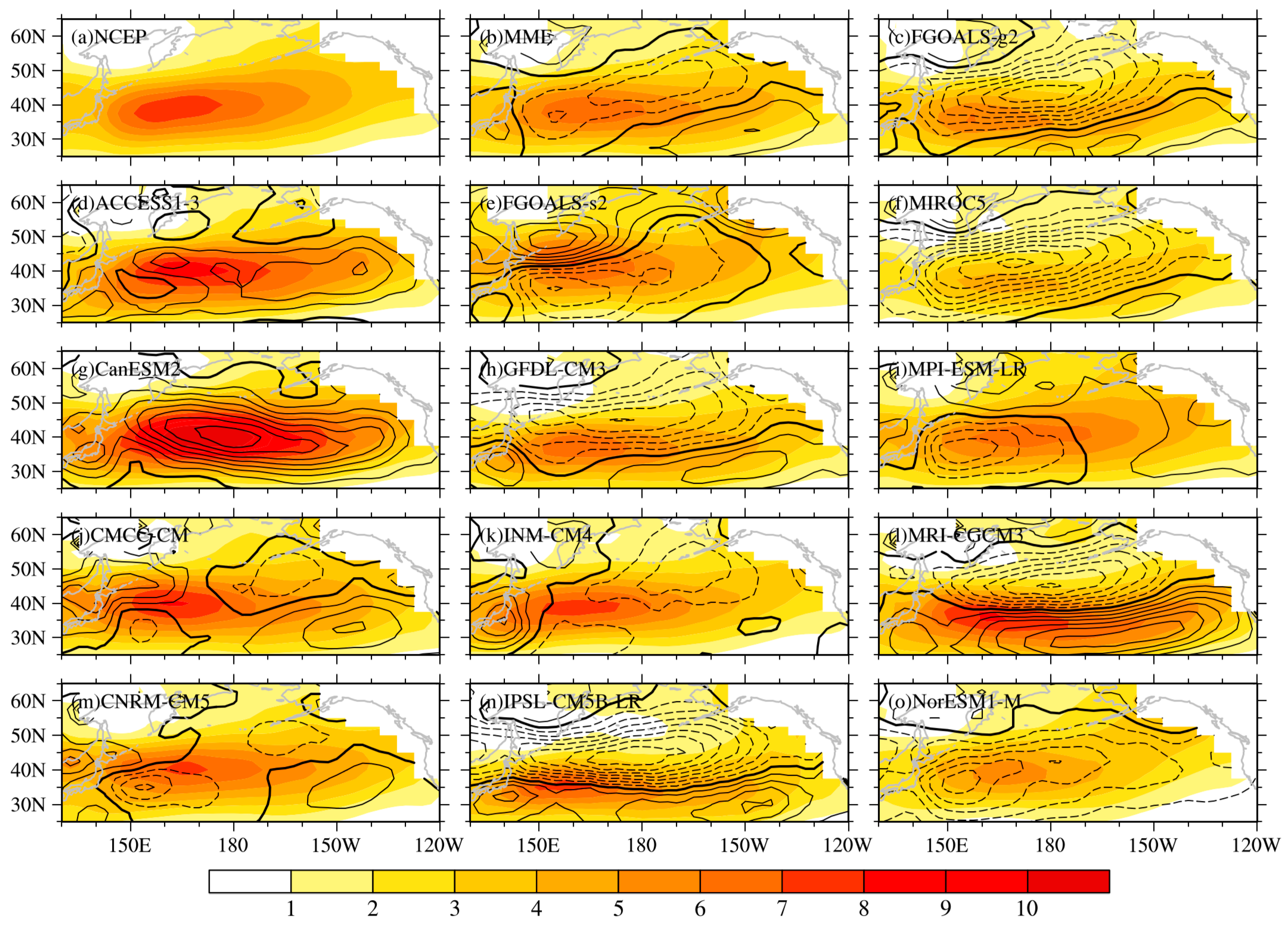
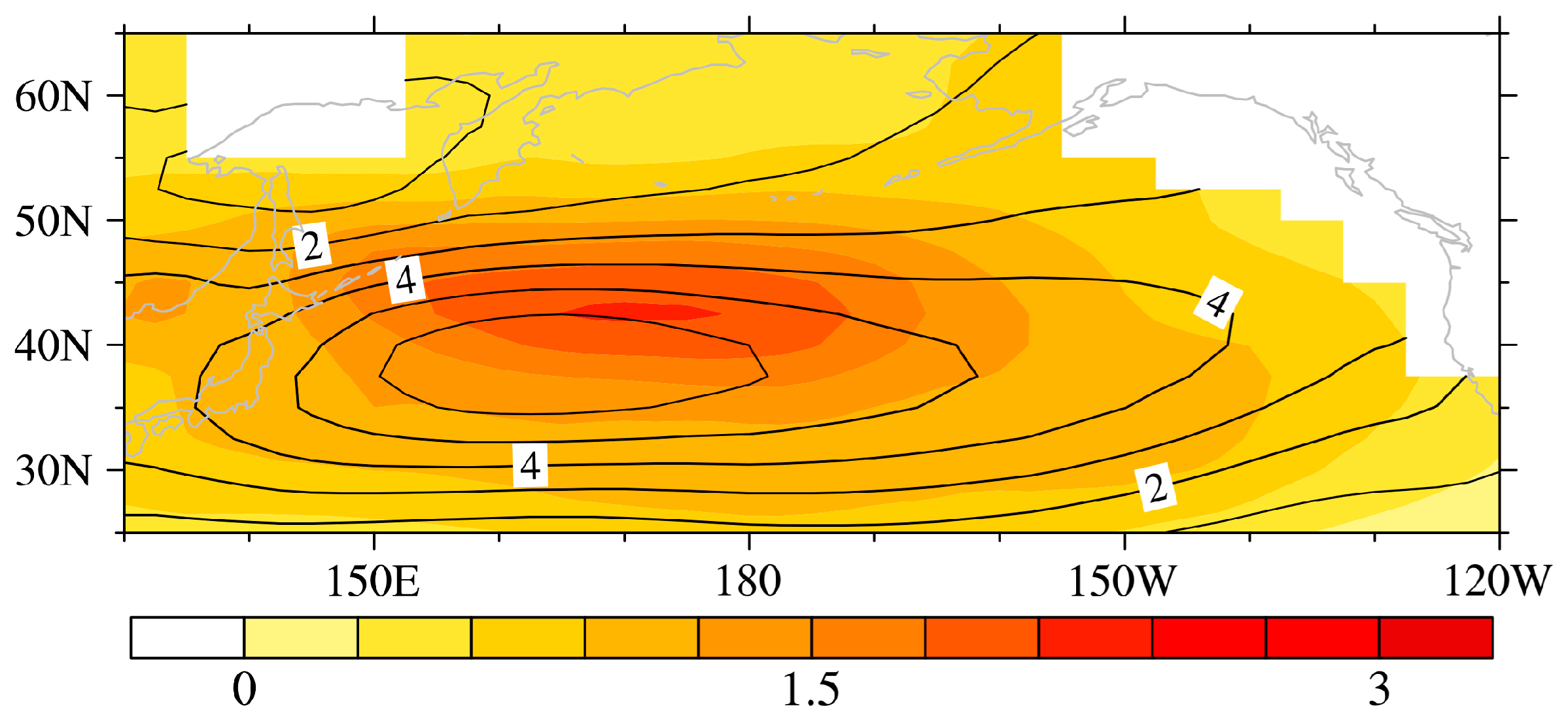
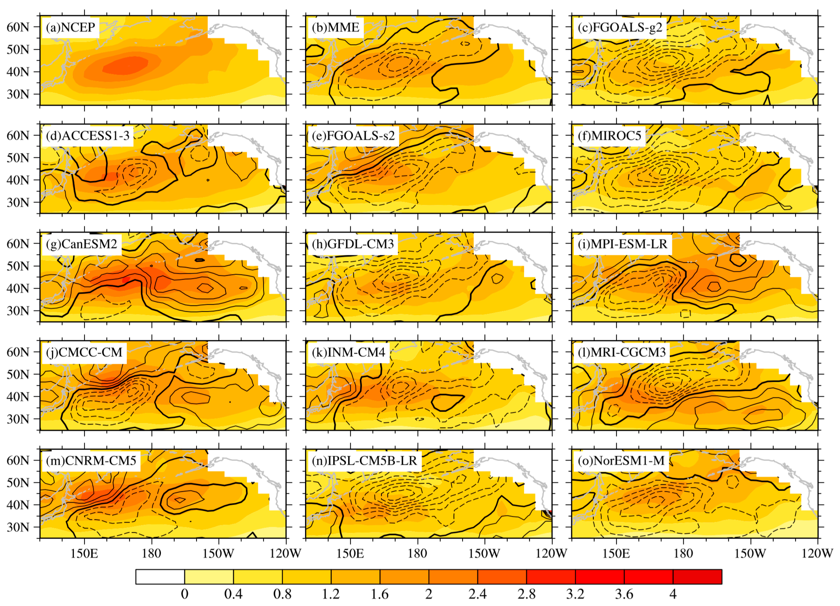
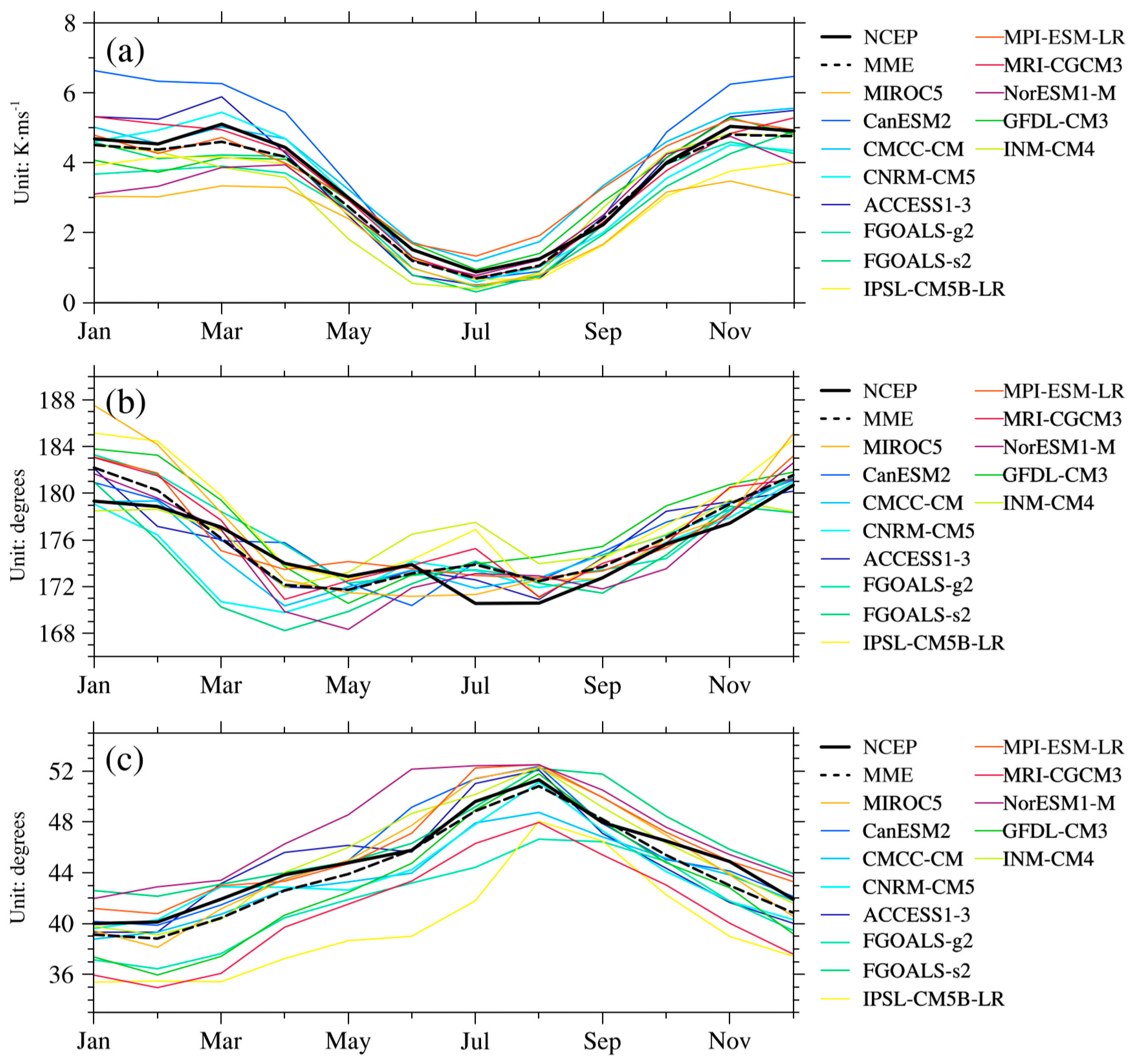
3.1. Climatology
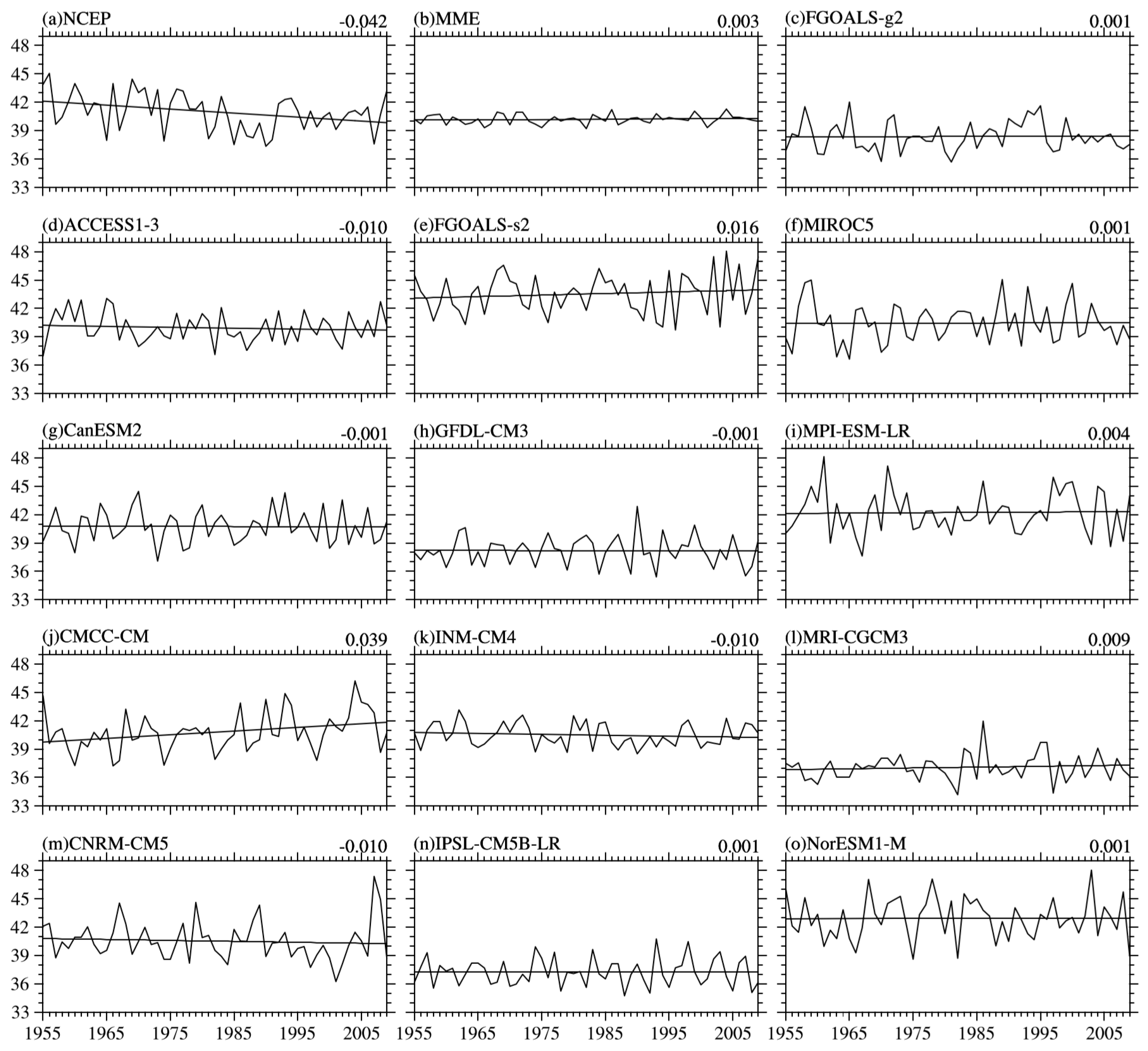
3.2. Interannual Variation of WNPST Strength
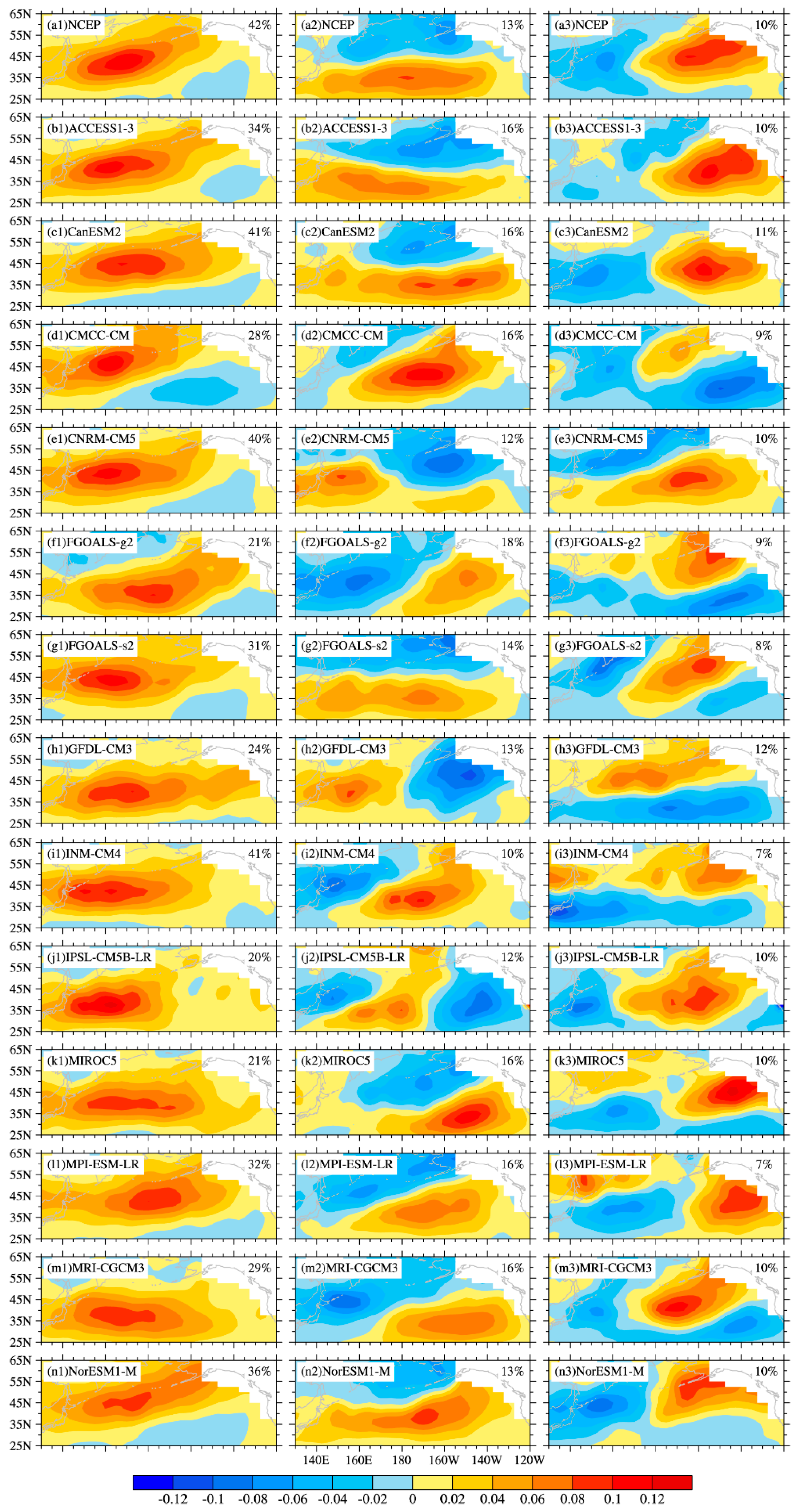
3.3. Spatial Modes
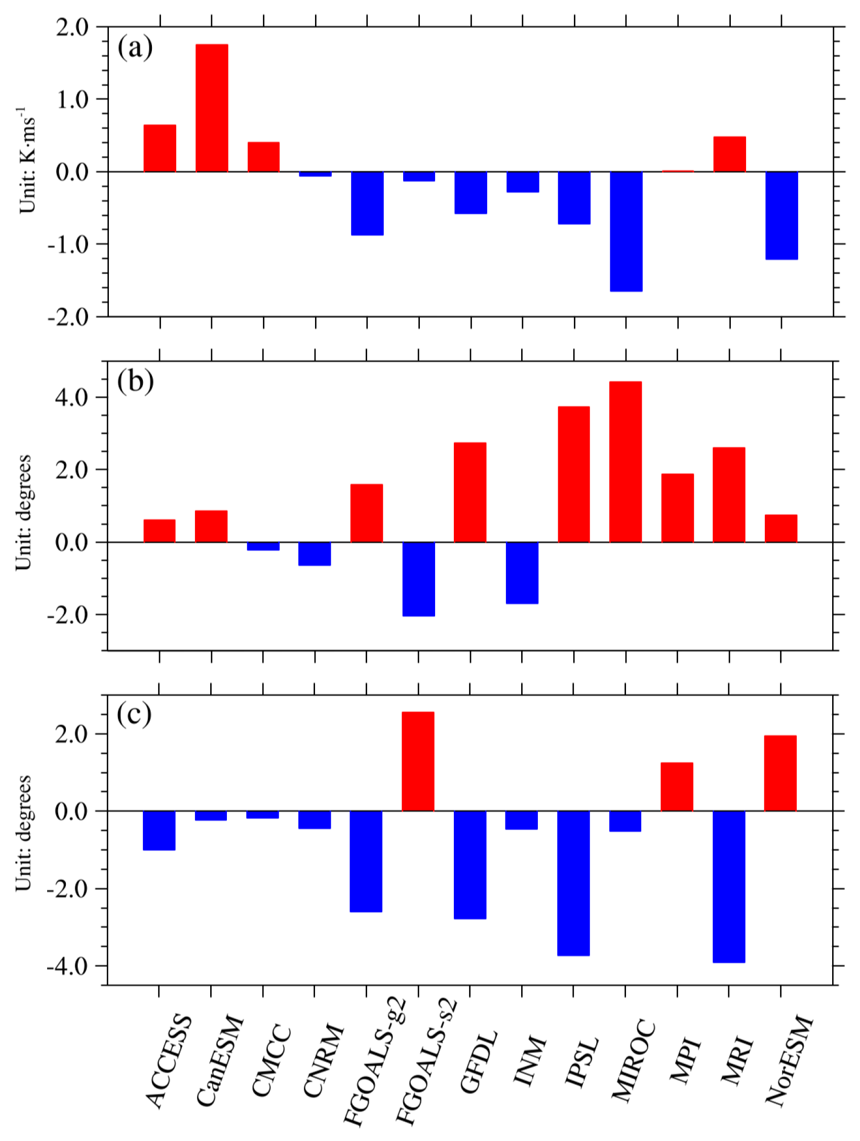
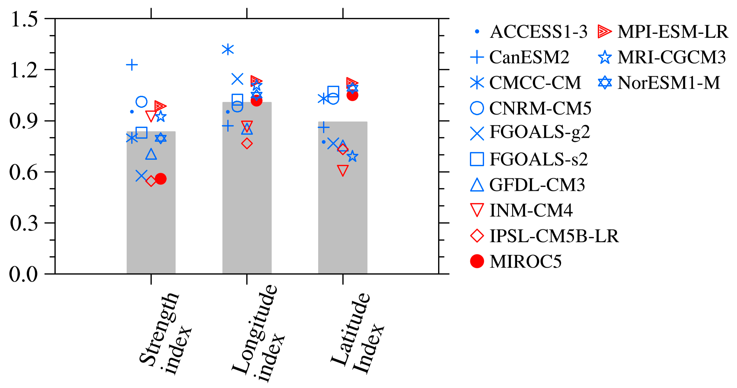
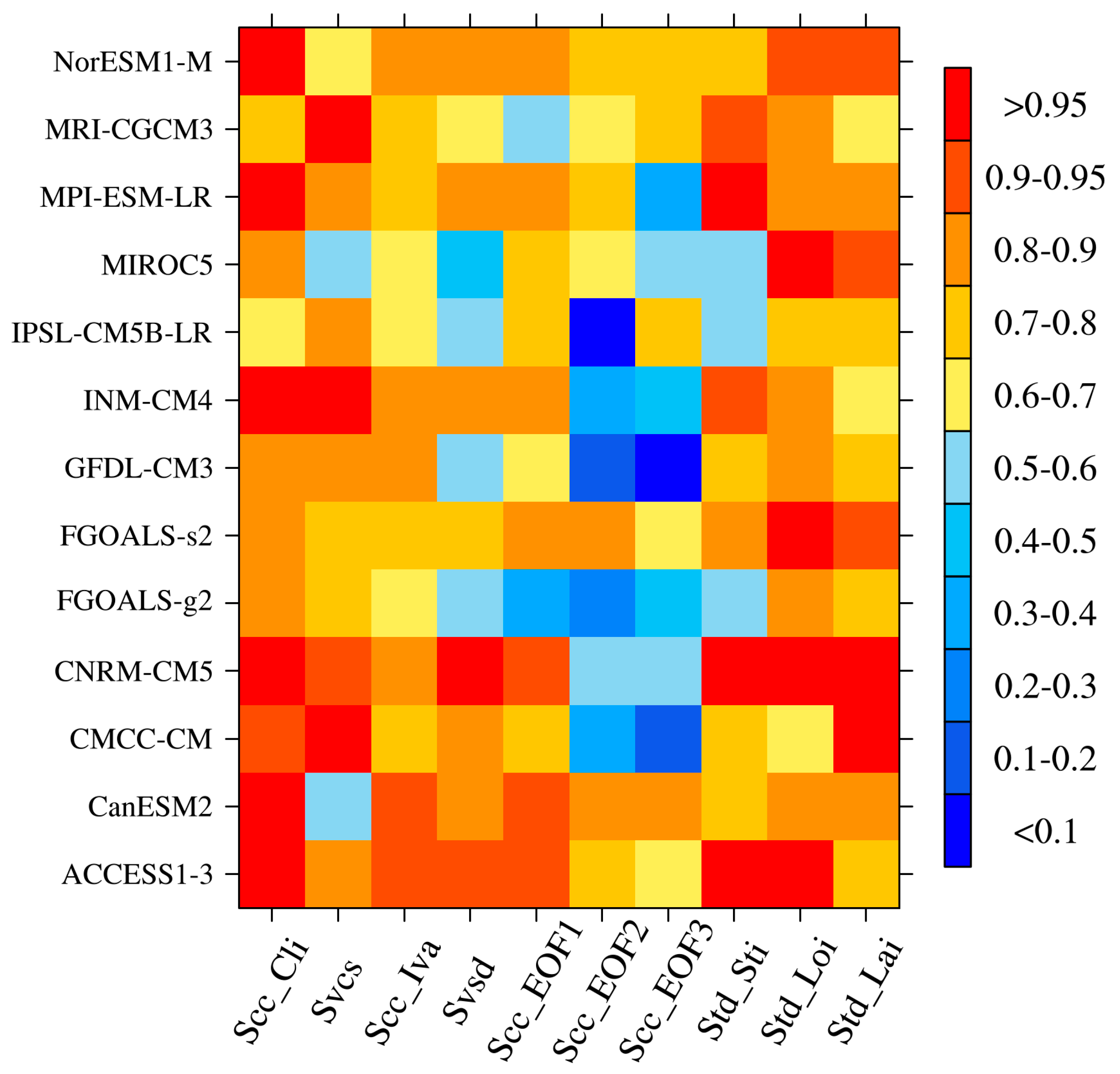
3.4. WNPST Indices
4. Summary
Acknowledgments
Author Contributions
Conflicts of Interest
References
- Blackmon, M.L.; Wallace, J.M.; Lau, N.C.; Mullen, S.L. An observational study of the Northern Hemisphere wintertime circulation. J. Atmos. Sci. 1977, 34, 1040–1053. [Google Scholar] [CrossRef]
- Nakamura, H. Midwinter suppression of baroclinic wave activity in the Pacific. J. Atmos. Sci. 1992, 49, 1629–1642. [Google Scholar] [CrossRef]
- Chang, E.K.M. Downstream development of baroclinic waves as inferred from regression analysis. J. Atmos. Sci. 1993, 50, 2038–2053. [Google Scholar] [CrossRef]
- Chang, E.K.M.; Fu, Y. Interdecadal variations in Northern Hemisphere winter storm track intensity. J. Clim. 2002, 15, 642–658. [Google Scholar] [CrossRef]
- Booth, J.F.; Kwon, Y.O.; Ko, S.; Small, R.J.; Msadek, R. Spatial Patterns and Intensity of the Surface Storm Tracks in CMIP5 Models. J. Clim. 2017, 30, 4965–4981. [Google Scholar] [CrossRef]
- Nakamura, H.; Sampe, T. Trapping of synoptic-scale disturbances into the North-Pacific subtropical jet core in midwinter. Geophys. Res. Lett. 2002, 29, 8-1–8-4. [Google Scholar] [CrossRef]
- Chang, E.K.M. Assessing the increasing trend in Northern Hemisphere winter storm track activity using surface ship observations and a statistical storm track model. J. Clim. 2007, 20, 5607–5628. [Google Scholar] [CrossRef]
- Lee, Y.Y.; Lim, G.H.; Kug, J.S. Influence of the East Asian winter monsoon on the storm track activity over the North Pacific. J. Geophys. Res. 2010, 115, D09102. [Google Scholar] [CrossRef]
- Deng, Y.; Jiang, T. Intraseasonal modulation of the North Pacific storm track by tropical convection in boreal winter. J. Clim. 2011, 24, 1122–1137. [Google Scholar] [CrossRef]
- Lee, Y.Y.; Lim, G.H. Dependency of the North Pacific winter storm tracks on the zonal distribution of MJO convection. J. Geophys. Res. 2012, 117, D14101. [Google Scholar] [CrossRef]
- Lee, Y.Y.; Kug, J.S.; Lim, G.H.; Watanabe, M. Eastward shift of the Pacific/North American pattern on an interdecadal time scale and an associated synoptic eddy feedback. Int. J. Climatol. 2011, 32, 1128–1134. [Google Scholar] [CrossRef]
- Straus, D.M.; Shukla, J. Variations of midlatitude transient dynamics associated with ENSO. J. Atmos. Sci. 1997, 54, 777–790. [Google Scholar] [CrossRef]
- Trenberth, K.E.; Hurrell, J.W. Decadal atmosphere-ocean variations in the Pacific. Clim. Dyn. 1994, 9, 303–319. [Google Scholar] [CrossRef]
- Hoskins, B.J.; Hodges, K.I. New perspectives on the Northern Hemisphere winter storm tracks. J. Atmos. Sci. 2002, 59, 1041–1061. [Google Scholar] [CrossRef]
- Booth, J.F.; Thompson, L.A.; Patoux, J.; Kelly, K.A.; Dickinson, S. The signature of the midlatitude tropospheric storm tracks in the surface winds. J. Clim. 2010, 23, 1160–1174. [Google Scholar] [CrossRef]
- Held, I.M.; Lyons, S.W.; Nigam, S. Transients and the extratropical response to El Niño. J. Atmos. Sci. 1989, 163–174. [Google Scholar] [CrossRef]
- Nakamura, H.; Izumi, T.; Sampe, T. Interannual and decadal modulations recently observed in the Pacific storm track activity and East Asian winter monsoon. J. Clim. 2002, 15, 1855–1874. [Google Scholar] [CrossRef]
- Yin, J.H. A consistent poleward shift of the storm tracks in simulations of 21st century climate. Geophys. Res. Lett. 2005, 32, L18701. [Google Scholar] [CrossRef]
- Ulbrich, U.; Pinto, J.G.; Kupfer, H.; Leckebusch, G.C.; Spangehl, T.; Reyers, M. Changing Northern Hemisphere storm tracks in an ensemble of IPCC climate change simulations. J. Clim. 2008, 21, 1669–1679. [Google Scholar] [CrossRef]
- Cai, M.; Mak, M. Symbiotic relation between planetary and synopticscale waves. J. Atmos. Sci. 1990, 47, 2953–2968. [Google Scholar] [CrossRef]
- Chang, E.K.M. An idealized nonlinear model of the Northern Hemisphere winter storm tracks. J. Atmos. Sci. 2006, 63, 1818–1839. [Google Scholar] [CrossRef]
- Chang, E.K.M.; Guo, Y.J. Dynamics of the stationary anomalies associated with the interannual variability of the midwinter Pacific storm track-The roles of tropical heating and remote eddy forcing. J. Atmos. Sci. 2007, 64, 2442–2461. [Google Scholar] [CrossRef]
- Yao, Y.; Zhong, Z.; Yang, X.Q. Numerical experiments of the storm track sensitivity to oceanic frontal strength within the Kuroshio/Oyashio Extensions. J. Geophys. Res. Atmos. 2016, 121, 2888–2900. [Google Scholar] [CrossRef]
- Nakamura, H.; Sampe, T.; Goto, A.; Ohfuchi, W.; Xie, S.P. On the importance of midlatitude oceanic frontal zones for the mean state and dominant variability in the tropospheric circulation. Geophys. Res. Lett. 2008, 35, L15709. [Google Scholar] [CrossRef]
- Nakamura, H.; Sampe, T.; Tanimoto, Y.; Shimpo, A. Observed associations among storm tracks, jet streams and midlatitude oceanic fronts. Geophys. Monogr. Ser. 2004, 147, 329–345. [Google Scholar] [CrossRef]
- Taylor, K.E.; Stouffer, R.J.; Meehl, G.A. An overview of CMIP5 and the experiment design. Bull. Am. Meteorol. Soc. 2012, 93, 485–498. [Google Scholar] [CrossRef]
- Gong, H.; Wang, L.; Chen, W.; Wu, R.; Wei, K.; Cui, X. The Climatology and Interannual Variability of the East Asian Winter Monsoon in CMIP5 Models. J. Clim. 2014, 27, 1659–1678. [Google Scholar] [CrossRef]
- Chang, E.K.M.; Guo, Y.; Xia, X. CMIP5 multi-model ensemble projection of storm track change under global warming. J. Geophys. Res. 2012, 117, D23118. [Google Scholar] [CrossRef]
- Chang, E.K.M.; Guo, Y.; Xia, X.; Zheng, M. Storm track activity in IPCC AR4/CMIP3 model simulations. J. Clim. 2013, 26, 246–260. [Google Scholar] [CrossRef]
- Li, Y.; Zhu, W.; Wei, J. Reappraisal and improvement of winter storm track indices in the North Pacific. Chin. J. Atmos. Sci. 2010, 34, 1001–1010. (In Chinese) [Google Scholar]
- North, G.; Bell, T.; Cahalan, R.; Moeng, F. Sampling errors in the estimation of empirical orthogonal functions. Mon. Weather Rev. 1982, 110, 699–706. [Google Scholar] [CrossRef]
- Timm, O.; Diaz, H.F. Synoptic-Statistical Approach to Regional Downscaling of IPCC Twenty-First-Century Climate Projections: Seasonal Rainfall over the Hawaiian Islands. J. Clim. 2009, 22, 4261–4280. [Google Scholar] [CrossRef]
- Taylor, K.E. Summarizing multiple aspects of model performance in a single diagram. J. Geophys. Res. Atmos. 2001, 106, 7183–7192. [Google Scholar] [CrossRef]
- Jiang, D.B.; Tian, Z.P. East Asian monsoon change for the 21st century: results of CMIP3 and CMIP5 models. Chin. Sci. Bull. 2012, 58, 1427–1435. [Google Scholar] [CrossRef]
- Ren, X.J.; Yang, X.Q.; Han, B.; Xu, G.Y. Storm track variations in the North Pacific in winter season and the coupled pattern with the midlatitude atmosphere-ocean system. Chin. J. Geophys. 2007, 50, 94–103. (In Chinese) [Google Scholar] [CrossRef]


| Model Name | Modeling Group | Atmospheric Resolution (Longitude × Latitude) |
|---|---|---|
| ACCESS1-3 (Australian Community Climate and Earth-System Simulator, version 1–3) | CSIRO and BoM, Australia | 192 × 145 |
| CanESM2 (Second Generation Canadian Earth System Model) | CCCma, Canada | 128 × 64 |
| CMCC-CM (Centro Euro-Mediterraneo per I Cambiamenti Climatici Climate Model) | CMCC, Italy | 480 × 240 |
| CNRM-CM5 (Centre National de Recherches Météorologiques Coupled Global Climate Model, version 5) | Centre National de RecherchesM´et´eorologiques and Centre Europeen de Recherche et Formation Avancees en Calcul Scientifique, France | 256 × 128 |
| FGOALS-g2 (Flexible Global Ocean-Atmosphere-Land System Model (FGOALS) gridpoint, version 2) | LASG, IAP, Chinese Academy of Sciences, China | 128 × 64 |
| FGOALS-s2 (FGOALS, second spectral version) | LASG, IAP, Chinese Academy of Sciences, China | 128 × 108 |
| GFDL-CM3 (Geophysical Fluid Dynamics Laboratory Climate Model, version 3) | GFDL, NOAA, United States | 144 × 90 |
| INM-CM4 (Institute of Numerica1 Mathematics Climate Model version 4) | Institute for Numerical Mathematics, Russia | 180 × 120 |
| IPSL-CM5B-LR (L’Institut Pierre-Simon Laplace Coupled Model, version 5B, coupled with NEMO, low resolution) | IPSL, France | 96 × 96 |
| MIROC5 (Model for Interdisciplinary Research on Climate, version 5) | Atmosphere and Ocean Research Institute (University of Tokyo), National Institute for Environmental Studies, and Japan Agency for Marine-Earth Science and Technology, Japan | 256 × 128 |
| MPI-ESM-LR (Max Planck Institute Earth System Model, low resolution) | MPI for Meteorology, Germany | 192 × 96 |
| MRI-CGCM3 (Meteorological Research Institute Coupled Atmosphere–Ocean General Circulation Model, version 3) | Meteorological Research Institute, Japan | 320 × 160 |
| NorESM1-M (Norwegian Earth System Model, version 1 (intermediate resolution)) | Norwegian Climate Centre, Norway | 144 × 96 |
| Model Name | EOF1 | EOF2 | EOF3 |
|---|---|---|---|
| ACCESS1-3 | 0.95 | 0.78 | 0.66 |
| CanESM2 | 0.90 | 0.85 | 0.87 |
| CMCC-CM | 0.72 | 0.34 (0.40) | 0.14 (0.67) |
| CNRM-CM5 | 0.93 | 0.52 (0.68) | 0.56 (0.72) |
| FGOALS-g2 | 0.38 | 0.28 (0.61) | 0.43 (0.71) |
| FGOALS-s2 | 0.88 | 0.86 | 0.63 |
| GFDL-CM3 | 0.68 | 0.11 (0.77) | 0.08 (0.89) |
| INM-CM4 | 0.88 | 0.38 (0.64) | 0.46 (0.70) |
| IPSL-CM5B-LR | 0.71 | 0.02 | 0.75 |
| MIROC5 | 0.72 | 0.62 | 0.57 |
| MPI-ESM-LR | 0.80 | 0.78 | 0.37 |
| MRI-CGCM3 | 0.51 | 0.63 | 0.74 |
| NorESM1-M | 0.84 | 0.74 | 0.80 |
| Model Name | Score |
|---|---|
| ACCESS1-3 | 0.63 |
| CanESM2 | 0.64 |
| CMCC-CM | 0.52 |
| CNRM-CM5 | 0.62 |
| FGOALS-g2 | 0.46 |
| FGOALS-s2 | 0.59 |
| GFDL-CM3 | 0.47 |
| INM-CM4 | 0.56 |
| IPSL-CM5B-LR | 0.43 |
| MIROC5 | 0.57 |
| MPI-ESM-LR | 0.56 |
| MRI-CGCM3 | 0.55 |
| NorESM1-M | 0.63 |
© 2018 by the authors. Licensee MDPI, Basel, Switzerland. This article is an open access article distributed under the terms and conditions of the Creative Commons Attribution (CC BY) license (http://creativecommons.org/licenses/by/4.0/).
Share and Cite
Yang, M.; Li, X.; Zuo, R.; Chen, X.; Wang, L. Climatology and Interannual Variability of Winter North Pacific Storm Track in CMIP5 Models. Atmosphere 2018, 9, 79. https://doi.org/10.3390/atmos9030079
Yang M, Li X, Zuo R, Chen X, Wang L. Climatology and Interannual Variability of Winter North Pacific Storm Track in CMIP5 Models. Atmosphere. 2018; 9(3):79. https://doi.org/10.3390/atmos9030079
Chicago/Turabian StyleYang, Minghao, Xin Li, Ruiting Zuo, Xiong Chen, and Liqiong Wang. 2018. "Climatology and Interannual Variability of Winter North Pacific Storm Track in CMIP5 Models" Atmosphere 9, no. 3: 79. https://doi.org/10.3390/atmos9030079