An Ensemble Mean and Evaluation of Third Generation Global Climate Reanalysis Models
by
 and
and
Jeffrey D. Auger
1,*, 
Sean D. Birkel
1,
Kirk A. Maasch
1,
Paul A. Mayewski
1 and
Keah C. Schuenemann
2 1
Climate Change Institute and School of Earth and Climate Sciences, University of Maine, Orono, ME 04473, USA
2
Department of Earth and Atmospheric Sciences, Metropolitan State University of Denver, Denver, CO 80204, USA
*
Author to whom correspondence should be addressed.
Atmosphere 2018, 9(6), 236; https://doi.org/10.3390/atmos9060236
Submission received: 9 February 2018
/
Revised: 14 June 2018
/
Accepted: 16 June 2018
/
Published: 19 June 2018
(This article belongs to the Special Issue Precipitation: Measurement and Modeling)
Abstract
:We have produced a global ensemble mean of the four third-generation climate reanalysis models for the years 1981–2010. The reanalysis system models used in this study are National Centers for Environmental Prediction (NCEP) Climate Forecast System Reanalysis (CFSR), European Centre for Medium-Range Weather Forecasts (ECMWF) Reanalysis Interim (ERA-I), Japan Meteorological Agency (JMA) 55-year Reanalysis (JRA-55), and National Aeronautics and Space Administration (NASA) Modern-Era Retrospective Analysis for Research and Applications (MERRA). Two gridded datasets are used as a baseline, for temperature the Global Historical Climatology Network (GHCN), and for precipitation the Global Precipitation Climatology Centre (GPCC). The reanalysis ensemble mean is used here as a comparison tool of the four reanalysis members. Meteorological fields investigated within the reanalysis models include 2-m air temperature, precipitation, and 500-hPa geopotential heights. Comparing the individual reanalysis models to the ensemble mean, we find that each perform similarly over large domains but exhibit significant differences over particular regions.
1. Introduction
Reanalysis models are numerical frameworks from which gridded solutions for past atmospheric states are obtained from the assimilation of historical meteorological observations. The first such model National Center for Environmental Prediction and National Center for Atmospheric Research (NCEP, NCAR, respectively) Reanalysis (R1) [1] provides meteorological outputs on a global domain, over the period of 1948–present, on a coarse 2.5° × 2.5° horizontal grid. A second generation of global climate reanalysis models, including European Centre for Medium-Range Weather Forecasts (ECMWF) 40-year Reanalysis (ERA-40) [2] and Japan Meteorological Agency (JMA) 25-year Reanalysis (JRA-25) [3], made improvements over R1, and subsequent reanalyses, by integrating satellite data, cloud motion winds (ERA-40), and wind profiles around tropical cyclones (JRA-25) on a finer resolution output of 1.125° × 1.125°. A third generation of global reanalysis models made significant advances in data assimilation and internal physics, computed at resolutions finer than 1° × 1°. These models are NCEP Climate Forecast System Reanalysis (CFSR) [4], ECMWF Reanalysis Interim (ERA-I) [5], JMA 55-year Reanalysis (JRA-55) [6], and NASA Modern-Era Retrospective Analysis for Research and Applications (MERRA) [7]. However, since the beginning of this analysis, a new version of National Aeronautics and Space Administration (NASA) MERRA has been released, MERRA-2 [8]. The aforementioned reanalysis products span from January 1979 to at least December 2017 (at the time of this study), with the exception of JRA-55 which begins January 1958. Each of the third generation models are considered state-of-the-art, but differences in meteorological outputs arise following different modeling approaches (refer to Table 1 for general model comparisons; refer also to the Overview & Comparison Tables at https://climatedataguide.ucar.edu/climate-data/atmospheric-reanalysis-overview-comparison-tables).
Reanalysis products are increasingly used for investigations into the changing climate. For example, Santer et al. [11] find a trend of increasing tropopause heights in ERA-40 linked to anthropogenic-forced warming, in agreement with climate model simulations and satellite data. Serreze et al. [12] compare vertical temperature and moisture profiles from CFSR, ERA-I, and MERRA to radiosonde station data within the Arctic, a data-sparse region where gridded output is heavily simulated. They find good agreement between the reanalyses and measured temperature and moisture trends, even though uncertainties are produced in both radiosonde data and reanalyses. Lindsay et al. [13] evaluated seven reanalysis models (at least one model per reanalysis generation) for the Arctic region and find that the third generation reanalyses (CFSR, ERA-I, and MERRA) provide the most significant correlations to observations, but with biases between the reanalyses for 2-m air temperature and other metrics. Chen et al. [14] examine variability between CFSR, ERA-I, JRA-55, and MERRA in the warm-season diurnal cycle over East Asia. They find that although these four reanalysis models reproduce the diurnal precipitation well over large spatial scales, individual models disagree considerably over regional scales. Chen et al. [14] also show that JRA-55 is in good agreement with observational data showing an increase in morning precipitation over their investigated domain. This same study determines that JRA-55 accurately reproduces wind speeds on the leeside of the Tibetan Plateau.
The above evaluations can be referred to as model-observation comparisons, where reanalysis model simulations are assessed by comparison to observations made by either satellite and/or station data. Here, we present an ensemble mean of the four leading reanalysis models—CFSR, ERA-I, JRA-55, and MERRA—and compare the individual reanalysis models against the ensemble mean to examine differences in the 2-m air temperature (T2m), precipitation, and 500-hPa geopotential height (Z500) fields. Spatial and time series comparisons are made with respect to the 30-year climate average period 1981–2010. The reanalysis ensemble mean should not be taken as “truth”, as our primary intention is to identify similarities and differences between the reanalysis models to provide baseline information for future studies. Although interannual variability correlations for T2m are strong on the global mean, we find significant differences in T2m between the reanalyses over many arid regions. There are also notable precipitation departures between the models in association with the Intertropical Convergence Zone (ITCZ). For T2m and precipitation, gridded observations—Global Historical Climatology Network (GHCN) and Global Precipitation Climatology Centre (GPCC)—are shown for baseline differences for each reanalysis model as well as the ensemble mean.
2. Experiments
Each reanalysis model can be found in month average file formats, which were used to produce the 1981–2010 averages. For CFSR, monthly files were found at the National Centers for Environmental Information (NCEI; www.ncdc.noaa.gov/data-access/model-data/model-datasets/climate-forecast-system-version2-cfsv2). Output from ERA-I and JRA-55 models were obtained from the NCAR Computational Information Systems Laboratory (CISL) Research Data Archive (RDA; http://rda.ucar.edu) under ds627.1 and ds628.1, respectively. Monthly files for MERRA were obtained from the NASA Modeling and Assimilation Data and Information Services Center (MDISC; http://disc.sci.gsfc.nasa.gov/mdisc).
The unprocessed outputs for each reanalysis model in this study are on different horizontal grids (Table 1). For simplicity, all model output fields were regridded to the same regular 0.5° × 0.5° latitude-longitude grid matching that of CFSR. Although it is most common to regrid to the lowest resolution of a model suite, the choice to use a finer common grid does not alter interpretations on the large-scale features reported here. Regridding was done using bilinear interpolation from the Earth System Modeling Framework (ESMF) software embedded within NCAR Command Language (NCL). Once regridded, netCDF files were produced for monthly, seasonal, and annual averages for each year and reanalysis product. The 1981–2010 climate average was created, again, for each month, season, and total. The reanalysis ensemble was generated by averaging monthly, seasonal, and annual means of the regridded CFSR, ERA-I, JRA-55, and MERRA outputs produced as explained above.
Gridded datasets are used in this study as a baseline for the comparisons. For T2m, GHCN version 3 (https://data.nodc.noaa.gov/cgi-bin/iso?id=gov.noaa.ncdc:C00839) [15,16] gridded dataset is used. The GHCN output is already on a 0.5° × 0.5° latitude-longitude grid; however, the grid cells do not match that of the regridded reanalysis output (the upper-left corner of the array is 89.75° N and 0.25° E). Thus, it was necessary to regrid GHCN to start the upper-left corner at 90° N and 0° E to match the 0.5° × 0.5° latitude-longitude grid. As a baseline for precipitation, the Global Precipitation Climatology Centre (GPCC; https://www.esrl.noaa.gov/psd/data/gridded/data.gpcc.html) [17] files are used. Similar to GHCN, GPCC output is on a 0.5° × 0.5° latitude-longitude grid with the upper-left corner matching as well. The same regridding scheme was applied to GPCC output for comparisons to reanalyses. As with the reanalyses, 30-year mean files were made for the period of 1981–2010.
3. Results
3.1. Two-Meter Air Temperature
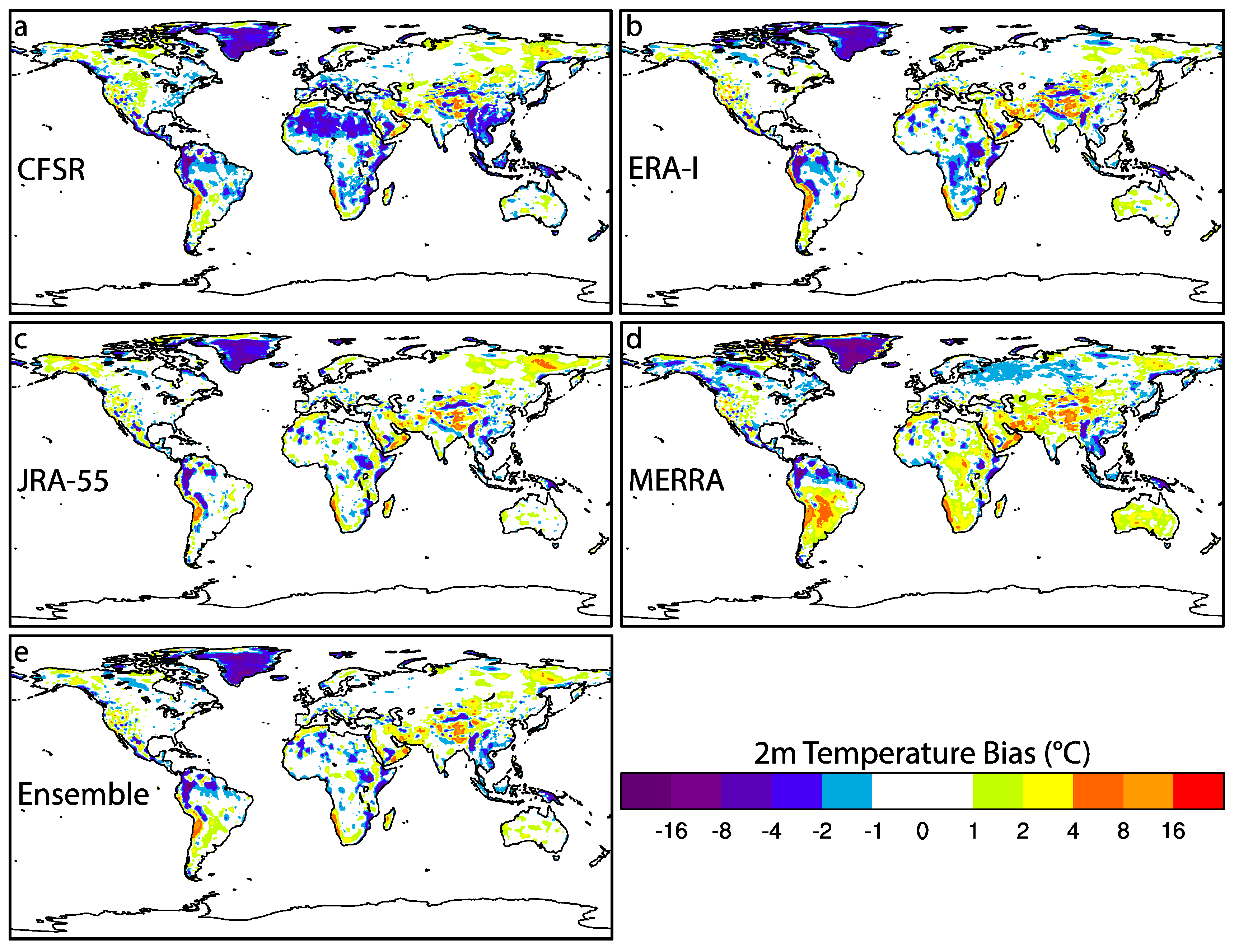
For the T2m (Figure 1) baseline we show each reanalysis (panels a–d) and the ensemble mean (panel e) subtract GHCN. It is evident that where observations are scarce there are major differences between the reanalyses/ensemble and GHCN output, such as in Greenland, central South America, Sahara Desert, and the Himalayas. Differences reach over 8 °C is some of these regions. Conversely, where observations are available for the duration of the reanalysis models, the outputs are closer to GHCN, as expected. The average differences between the reanalyses and GHCN range from −0.42 °C (CFSR) to 0.23 °C (MERRA) with JRA-55 having the smallest average difference at −0.03 °C over the 1981–2010 period. The ensemble mean is only slightly larger than JRA-55 at −0.09 °C.
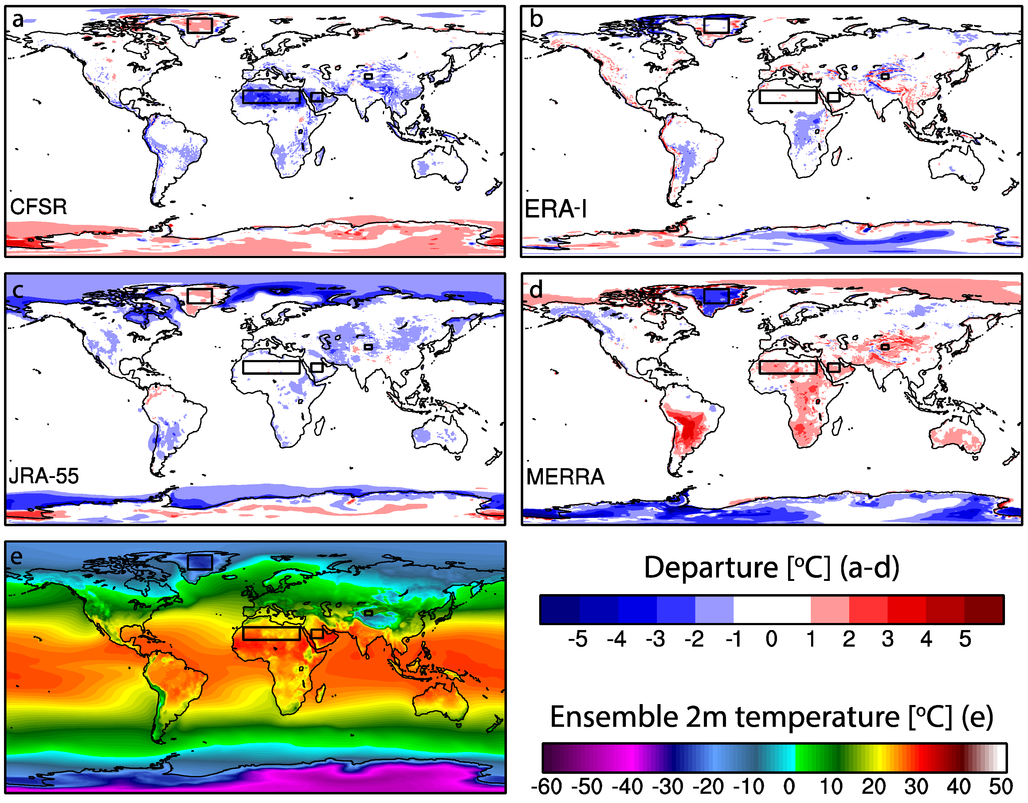
Global T2m differences between the reanalysis models and the ensemble mean (Figure 2) arise primarily near the poles, with slight departures from the mean generally in locations where observations are relatively scarce. For example, CFSR affords a negative 2–3 °C difference over the desert belts in Africa and the Middle East (i.e., Sahara, Sahel, and Saudi Arabia), while ERA-I shows most differences, about negative 1 °C, in Arctic Canada and East Antarctica. From JRA-55, T2m generally compares well with the ensemble mean overall with negative departures from the mean over the Arctic and Southern Oceans. Last, from MERRA, T2m is generally warmer than the mean over most of Africa, Australia, Central Asia, and South America.
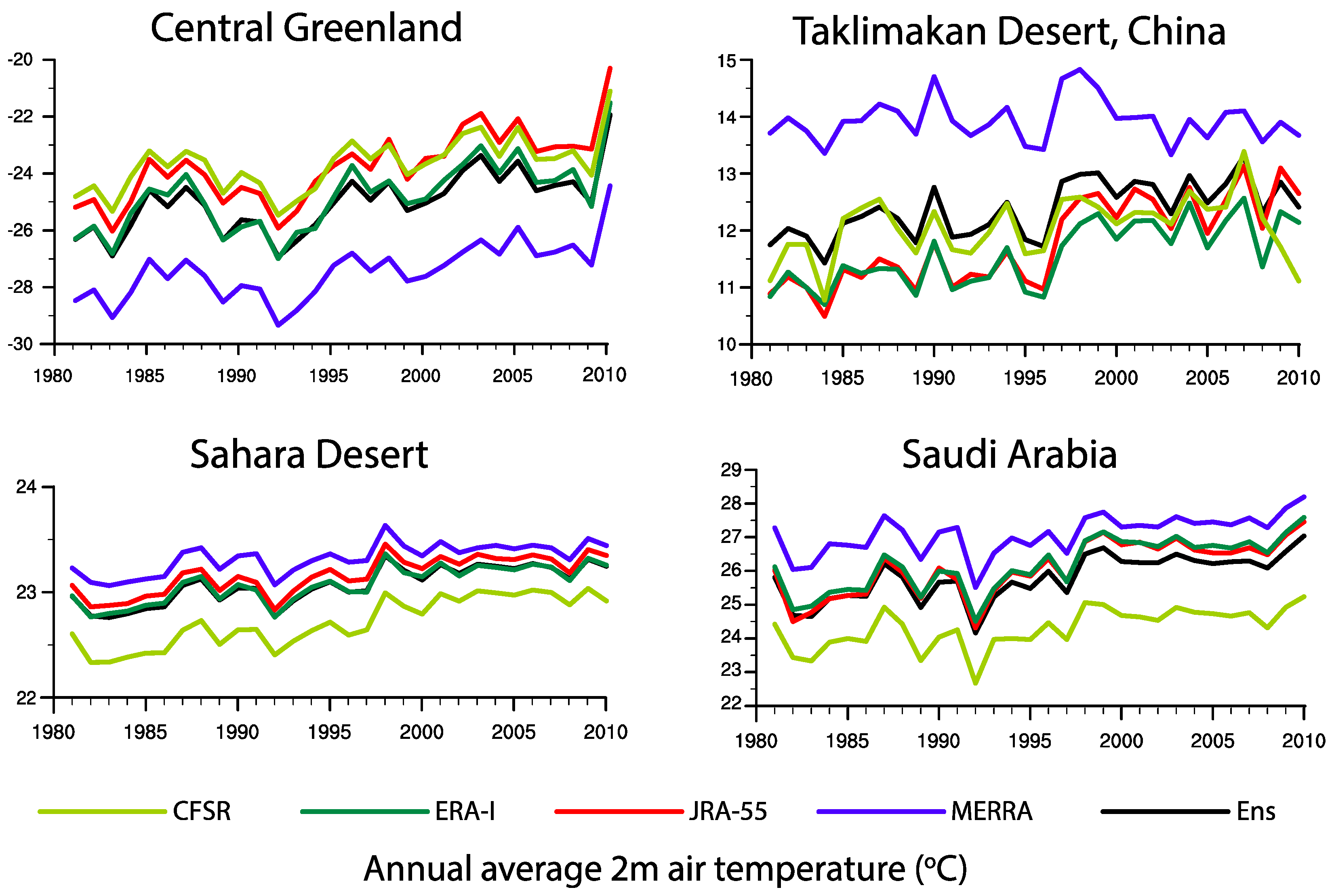
Time series of T2m during the 30-year study period over desert regions (black boxes in Figure 2) can be found in Figure 3. Interannual variability between the reanalyses agree well for each region (r > 0.8). The range of time series correlations across the smallest desert analyzed in this study, the Taklimakan Desert, China, is larger (0.41 < r < 0.97) than that of the correlation coefficient ranges for the Sahara Desert, Saudi Arabia, and Central Greenland (0.91 < r < 0.99, 0.94 < r < 0.99, and 0.95 < r < 0.99, respectively). The topography surrounding the Taklimakan Desert differs much more than that of the other deserts referred to here, which could explain the variability in correlations found between the reanalyses.
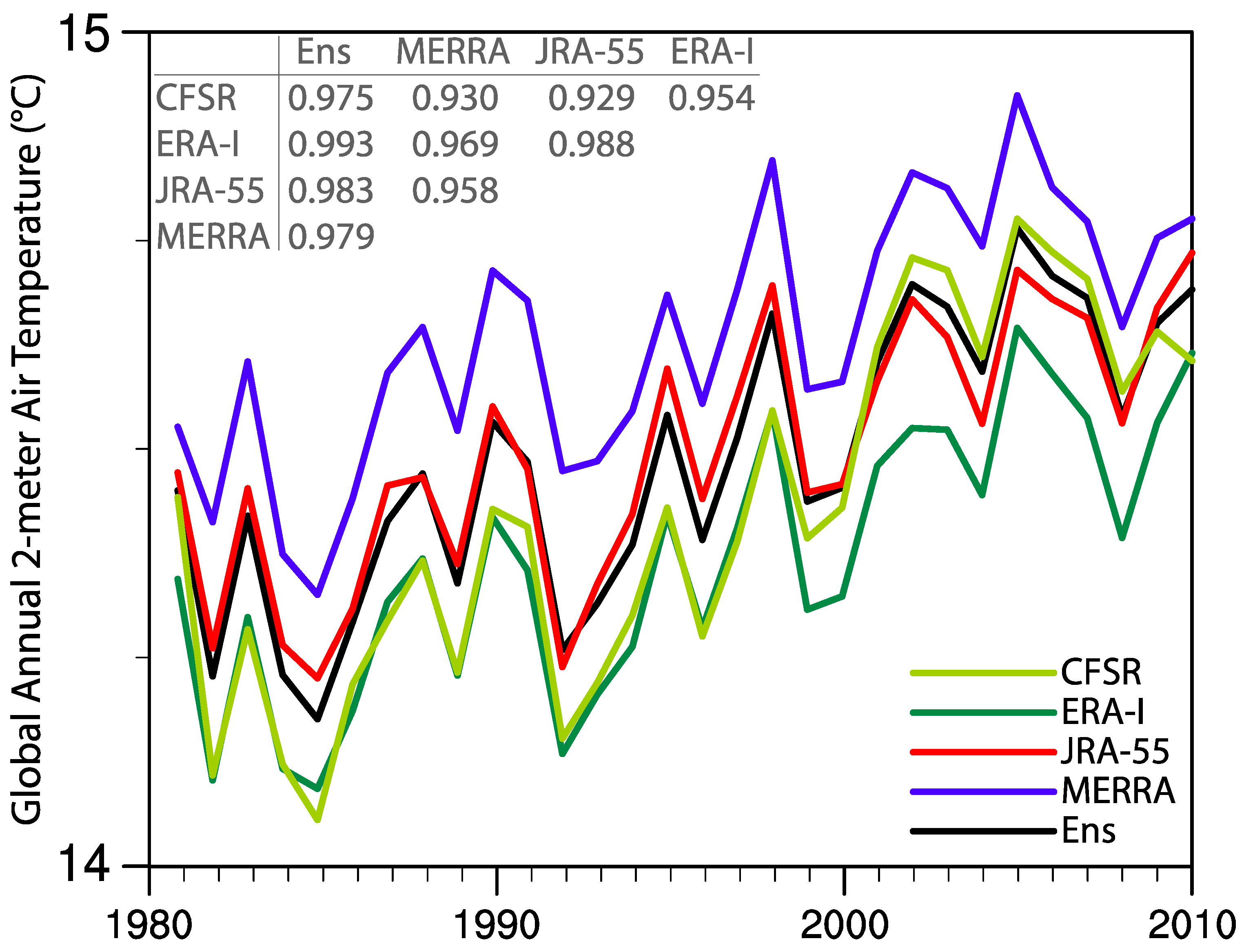
Figure 4 shows the T2m time series with accompanied correlation coefficients over the global domain. Note that all reanalysis-ensemble correlations are greater than 0.97. Reanalysis-reanalysis T2m correlations are also high, with the lowest being between CFSR and JRA-55 at 0.93. ERA-I shows the highest correlation against the ensemble mean at 0.99 with an average T2m difference of about −0.10 °C compared to that of the ensemble mean. MERRA T2m has the highest average deviation from the ensemble of about +0.14 °C. The MERRA T2m time series curve does not intersect the other reanalysis curves making MERRA outputs consistently warmer than all other reanalyses. The JRA-55 T2m time series is closest to the ensemble mean with a mean departure of only −0.02 °C.
In order to compare T2m trends the derivative of 5-year running means is used for each reanalysis model. ERA-I, JRA-55, and MERRA display similar trends across the 1981–2010 period. However, CFSR yields a steeper increase in T2m during the 1997–2003 period, which can be seen in Figure 4. The CFSR T2m increase over the 1997–2003 period is 0.061 °C/year whereas the other reanalysis trends are less than 0.038 °C/year. The last year over the study period, 2010, CFSR deviates from the trend of the other three reanalyses (Figure 4).
For ocean-based 2-m temperature, the reanalyses generally agree well with the ensemble mean, which is to be expected as sea surface temperature (SST) strongly influences T2m. The largest departures from the mean arise over the Arctic and Southern Oceans in JRA-55 (Figure 2). As these regions are data-sparse, this is expected. However, this could also be due to differences in sea ice, as near-surface temperature is highly influenced by sea ice. Each reanalysis, except CFSR, uses a prescribed SST field interpolated from observations. CFSR incorporates a combination of versions 1 and 2 of the optimum interpolation (OI) methods for the period November 1981–present [18]. As for the January 1979–October 1981 period, SST fields are used from ERA-40. For further information on reanalyses and SST data sets and methods for CFSR, ERA-I, and MERRA, refer to Kumar et al. [19]. JRA-55 uses the Centennial in situ Observation-Based Estimates (COBE) SST data set [20].
3.2. Precipitation
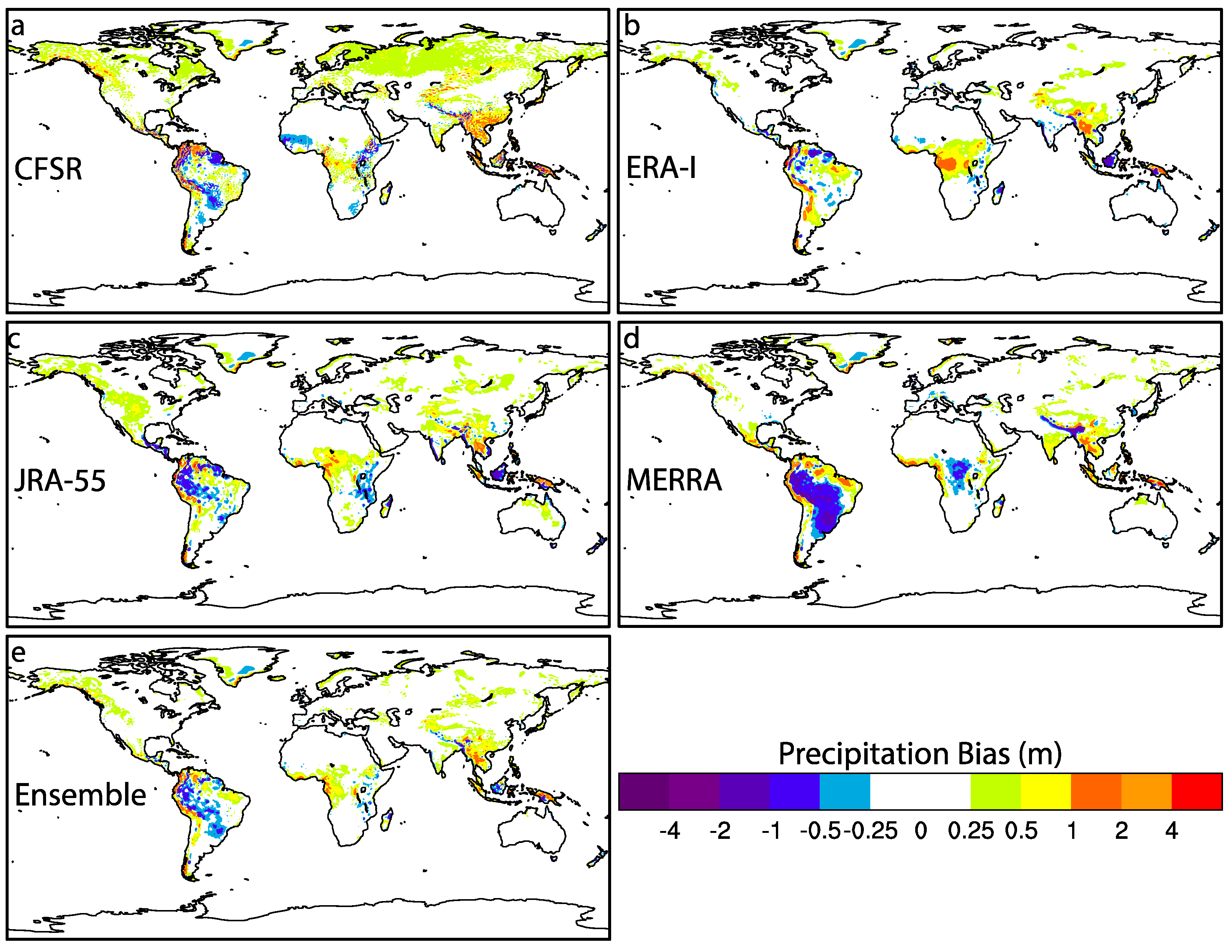
Using GPCC as the baseline for precipitation on land, we show differences between each reanalysis model and the ensemble mean, subtracting GPCC (Figure 5). It is evident that CFSR outputs more precipitation in the northern hemisphere with MERRA closer to GPCC. In South America, there are dryer outputs across all four reanalyses, with MERRA showing values over 1 m less than GPCC. Over the Himalayas, each reanalysis displays more precipitation with MERRA showing less on the southern slopes. The average differences across the domain are all positive, ranging from 0.04 m (MERRA) to 0.18 m (CFSR). However, MERRA precipitation being the closest to GPCC does not suggest it is “better” than the other reanalyses in this study, which is likely due to the large negative bias over South America. The ensemble mean average difference is 0.11 m.
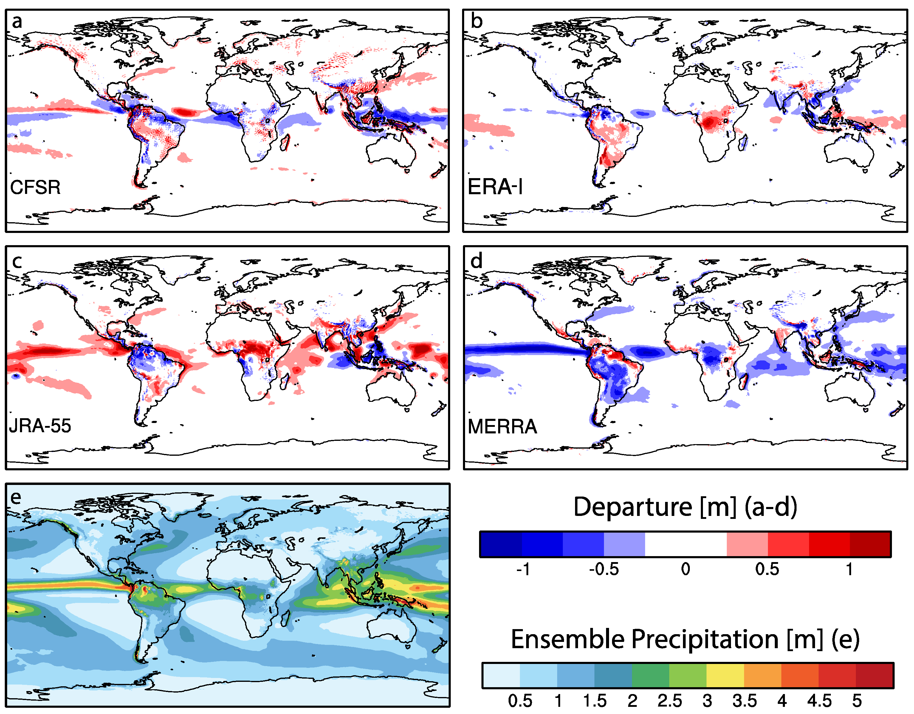
Difference plots between the reanalyses and ensemble mean for precipitation are shown in Figure 6. The spatial differences are noisy particularly along large mountain ranges (e.g., Himalayas) and near small islands that are resolved by the reanalyses (e.g., Philippines). Major differences are found along the ITCZ. In the eastern hemispheric tropics, CFSR and MERRA show less precipitation than the ensemble mean. JRA-55 shows precipitation values higher than the mean over the oceans and generally less than the mean over Indonesia, the Philippines, and Malaysia, as well as northern South America. The ERA-I precipitation departure is smaller than the other members along the eastern hemispheric tropics showing less precipitation over the islands and less than 0.5 m/year above the ensemble mean over the western tropical Pacific Ocean.
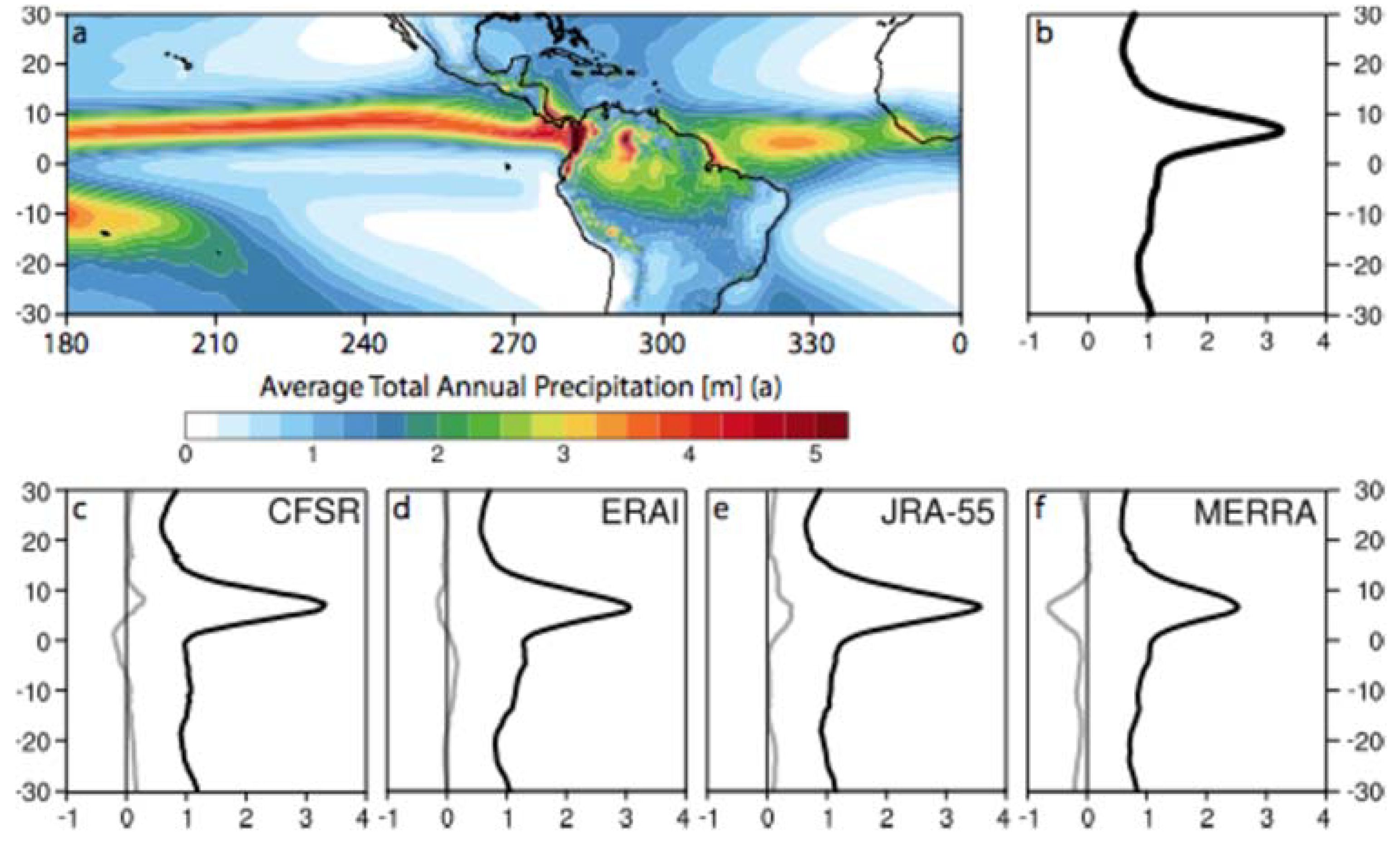
Figure 7 shows precipitation outputs over the western hemispheric tropics. CFSR and ERA-I in this region generally agree with the ensemble mean, whereas JRA-55 and MERRA deviate from the mean on the order of 0.47 and −0.67 m/year, respectively, at the peak of the zonal average. JRA-55 presents a much stronger precipitation belt while the zonal average from MERRA suggests a weaker precipitation belt, with respect to CFSR and ERA-I. Seasonal differences (Supplementary Figure S1) relative to the ensemble mean arise during the boreal summer (JJA) and fall (SON) months for JRA-55 and MERRA. The reanalysis models have poor agreement on the precipitation total in the ITCZ, but good agreement overall on timing of the seasonal shift of the ITCZ in the Western Hemisphere. The zonal average peaks for each reanalysis model fall within 1° latitude of the ensemble zonal average peak during the 1981–2010 climatology.
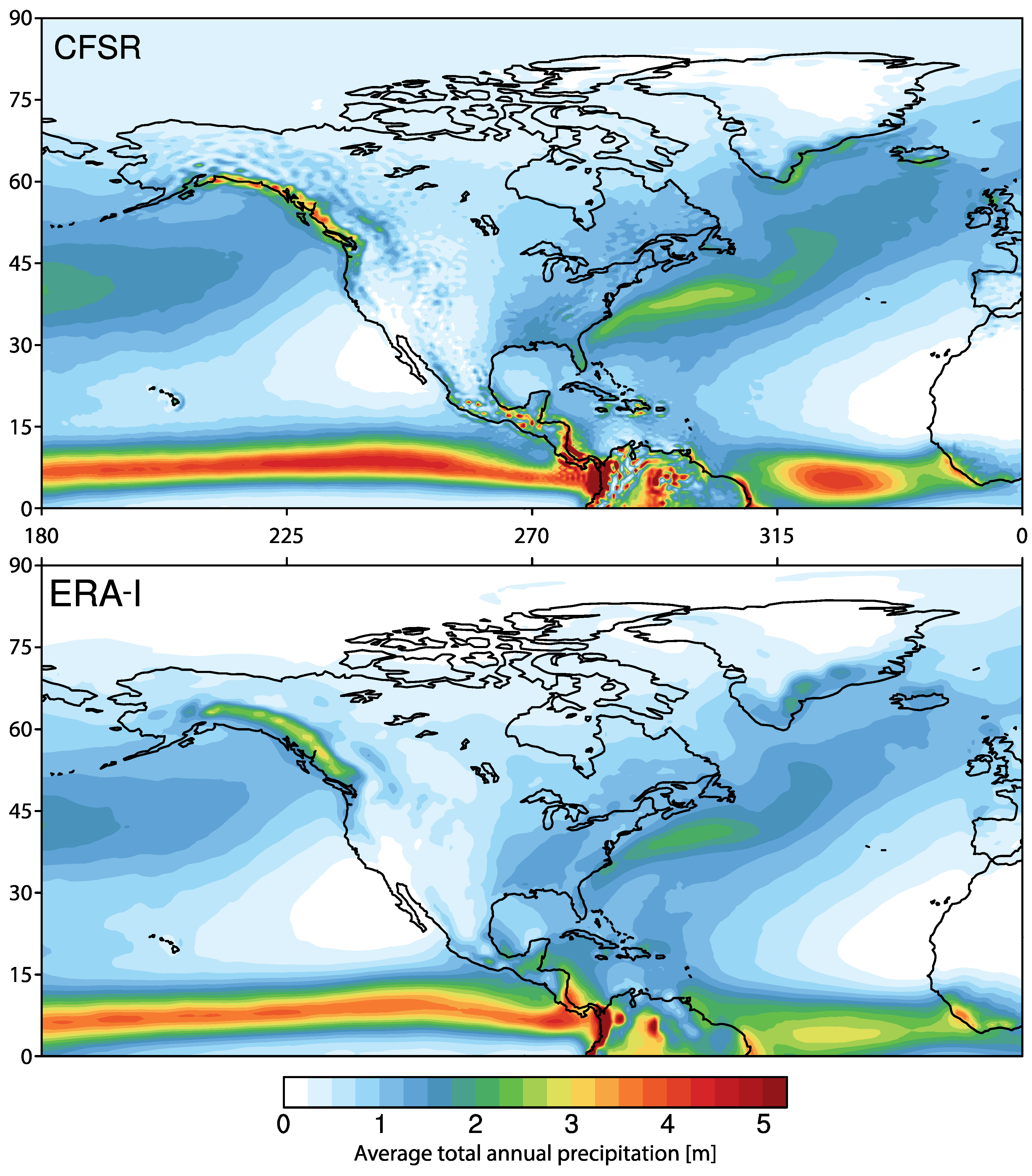
CFSR exhibits a specific weakness not found in the other models, where spherical harmonic artifacts appear in the precipitation (Figure 8) and T2m fields. These unrealistic features are not only found in sub-daily and monthly outputs, but also present in the climatological average, 1981–2010. Slight spherical harmonic artifacts in T2m and precipitation are present within the ensemble mean produced here as a result of the inclusion of CFSR.
3.3. Geopotential Heights at 500 hPa
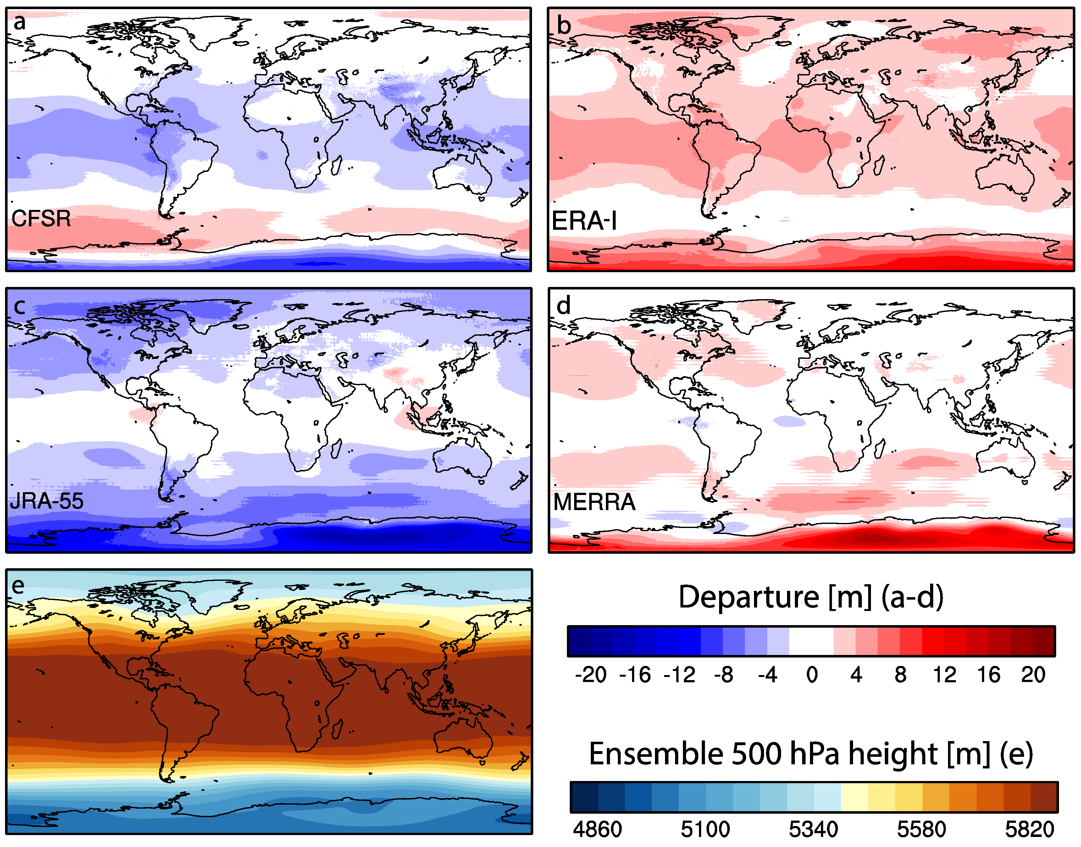
Geopotential heights at 500 hPa (Z500) generally agree across the four reanalyses with slight departures from the mean (±20 m) (Figure 9). The largest deviations are over Antarctica, where radiosonde observations are sparse, and therefore the models are poorly constrained. Above the friction layer, the free atmosphere becomes geostrophic, enabling model simulations to better approximate real-world observations.
4. Conclusions
In conclusion, three widely used atmospheric variables—T2m, precipitation, and Z500—are compared between each of the third-generation global climate reanalysis models—CFSR, ERA-I, JRA-55, and MERRA—and the respective ensemble mean of these reanalyses. While the four products generally agree on the large-scale, there are differences when examining regional-scale climatology. For example, we note that the precipitation belt in the ITCZ display differences between model solutions on the order of 13–20% (i.e., JRA-55 and MERRA, respectively) relative to the ensemble mean.
Over regional domains, T2m outputs for each reanalysis are shown to have large differences in extremely dry regions, such as polar ice sheets and low-latitude deserts. As examples, T2m over the Sahara and Saudi Arabia in CFSR (MERRA) is much lower (higher) with respect to the ensemble mean during the 1981–2010 period, whereas ERA-I and JRA-55 are generally in good accord with the mean (Figure 2 and Figure 3). Differences in these areas are most likely linked to scarce observation data. T2m correlations between the reanalysis models reveal strong agreement (Figure 4) for interannual variability, meaning that the models are in agreement on large-scale circulation processes over long temporal scales. Although, differences near the surface arise between the reanalysis model solutions, which could be attributed to any number of internal model differences, such as resolution, assimilation methods, observational input data error, land surface schemes, physics, etc. Future work on meteorological case studies will prove useful for improving seasonal, monthly, daily, and sub-daily reanalysis outputs and anomalies within the next generation of reanalysis products. Since most reanalysis differences occur at or near the surface, investigating the internal models and surface model schemes will bring reanalysis solutions closer to observations.
Supplementary Materials
Supplementary materials can be found at https://www.mdpi.com/2073-4433/9/6/236/s1.
Author Contributions
J.D.A., S.D.B., K.A.M., and P.A.M. conceived and designed the experiments; J.D.A. performed the experiments; J.D.A., S.D.B., K.A.M., P.A.M., and K.C.S. analyzed the data; J.D.A. wrote the paper.
Funding
This research received no external funding.
Acknowledgments
We thank Andrew Carlton (Pennsylvania State University) for manuscript suggestions and Mary Haley (NCAR) for NCL technical assistance. The authors would also like to thank the three anonymous reviewers for their insightful comments and suggestions which improved this paper. This work was supported by NSF awards PLR-1417640, P2C2-1401899, and P2C2-1600018; and Arcadia Fund of London AC3450. Individual reanalysis models and the ensemble mean produced here can be accessed using Climate Reanalyzer (https://cci-reanalyzer.org), a data visualization website developed by co-author S.D. Birkel for the Climate Change Institute at the University of Maine. This paper is part of the Arctic Futures Institute contribution series.
Conflicts of Interest
The authors declare no conflict of interest.
References
- Kalnay, E.; Kanamitsu, M.; Kistler, R.; Collins, W.; Deaven, D.; Gandin, L.; Iredell, M.; Saha, S.; White, G.; Woollen, J.; et al. The NCEP/NCAR 40-Year Reanalysis Project. Bull. Am. Meteorol. Soc. 1996, 77, 437–471. [Google Scholar] [CrossRef] [Green Version]
- Uppala, S.M.; Kållberg, P.W.; Simmons, A.J.; Andrae, U.; da Costa Bechtold, V.; Fiorino, M.; Gibson, J.K.; Haseler, J.; Hernandez, A.; Kelly, G.A.; et al. The ERA-40 re-analysis. Q. J. R. Meteorol. Soc. 2005, 131, 2961–3012. [Google Scholar] [CrossRef] [Green Version]
- Onogi, K.; Tsutsui, J.; Koide, H.; Sakamoto, M.; Kobayashi, S.; Hatsushika, H.; Matsumoto, T.; Yamazaki, N.; Kamahori, H.; Takahashi, K.; et al. The JRA-25 Reanalysis. J. Meteorol. Soc. Jpn. 2007, 85, 369–432. [Google Scholar] [CrossRef] [Green Version]
- Saha, S.; Moorthi, S.; Pan, H.-L.; Wu, X.; Wang, J.; Nadiga, S.; Tripp, P.; Kistler, R.; Woollen, J.; Behringer, D.; et al. The NCEP climate forecast system reanalysis. Bull. Am. Meteorol. Soc. 2010, 91, 1015–1057. [Google Scholar] [CrossRef]
- Dee, D.P.; Uppala, S.M.; Simmons, A.J.; Berrisford, P.; Poli, P.; Kobayashi, S.; Andrae, U.; Balmaseda, M.A.; Balsamo, G.; Bauer, P.; et al. The ERA Interim reanalysis: Configuration and performance of the data assimilation system. Q. J. R. Meteorol. Soc. 2011, 137, 553–597. [Google Scholar] [CrossRef]
- Kobayashi, S.; Ota, Y.; Harada, Y.; Ebita, A.; Moriya, M.; Onoda, H.; Onogi, K.; Kamahori, H.; Kobayashi, C.; Endo, H.; et al. The JRA-55 Reanalysis: General specification and basic characteristics. J. Meteorol. Soc. Jpn. 2015, 93, 5–48. [Google Scholar] [CrossRef]
- Rienecker, M.M.; Suarez, M.J.; Gelaro, R.; Todling, R.; Bachmeister, J.; Liu, E.; Bosilovich, M.G.; Schubert, S.D.; Takacs, L.; Kim, G.-K.; et al. MERRA: NASA’s Modern-era retrospective analysis for research and applications. J. Clim. 2011, 24, 3624–3648. [Google Scholar] [CrossRef]
- Gelaro, R.; McCarty, W.; Suárez, M.J.; Todling, R.; Molod, A.; Takacs, L.; Randles, C.A.; Darmenov, A.; Bosilovich, M.G.; Reichle, R.; et al. The Modern-Era Retrospective Analysis for Research and Applications, Version 2 (MERRA-2). J. Clim. 2017, 30, 5419–5454. [Google Scholar] [CrossRef]
- Chou, M.-D.; Suarez, M.J. A Solar Radiation Parameterization for Atmospheric Studies; NASA/TM-1999-104606; NASA: Greenbelt, MD, USA, 1999; Volume 15, 40p.
- Chou, M.-D.; Suarez, M.J.; Liang, X.Z.; Yan, M.M.-H. A Thermal Infrared Radiation Parameterization for Atmospheric Studies; NASA/TM-2001-104606; NASA: Greenbelt, MD, USA, 2001; Volume 19, 56p.
- Santer, B.D.; Wigley, T.M.L.; Simmons, A.J.; Kållberg, P.W.; Kelly, G.A.; Uppala, S.M.; Ammann, C.; Boyle, J.S.; Brüggemann, W.; Doutriaux, C.; et al. Identification of anthropogenic climate change using second-generation reanalysis. J. Geophys. Res. 2004, 109, D21104. [Google Scholar] [CrossRef]
- Serreze, M.C.; Barrett, A.P.; Stroeve, J. Recent changes in tropospheric water vapor over the Arctic as assessed from radiosondes and atmospheric reanalyses. J. Geophys. Res. 2012, 117, D10104. [Google Scholar] [CrossRef]
- Lindsay, R.; Wensnahan, M.; Schweiger, A.; Zhang, J. Evaluation of seven different atmospheric reanalysis products in the Arctic. J. Clim. 2014, 27, 2588–2606. [Google Scholar] [CrossRef]
- Chen, G.; Iwasaki, T.; Qin, H.; Sha, W. Evaluation of the warm-season diurnal variability over East Asia in recent reanalysis JRA-55, ERA Interim, NCEP CFSR, and NASA MERRA. J. Clim. 2014, 27, 5517–5537. [Google Scholar] [CrossRef]
- Lawrimore, J.H.; Menne, M.J.; Gleason, B.E.; Williams, C.N.; Wuertz, D.B.; Vose, R.S.; Rennie, J. Global Historical Climatology Network-Monthly (GHCN-M); version 3; NOAA National Centers for Environmental Information: Asheville, NC, USA, 2011.
- Peterson, T.C.; Vose, R.S. An overview of the Global Historical Climatology Network temperature database. Bull. Am. Meteorol. Soc. 1997, 78, 2837–2849. [Google Scholar] [CrossRef]
- Schneider, U.; Becker, A.; Finger, P.; Meyer-Christoffer, A.; Rudolf, B.; Ziese, M. GPCC Full Data Reanalysis Version 6.0 at 0.5°: Monthly Land-Surface Precipitation from Rain-Gauges Built on GTS-Based and Historic Data. Theor. Appl. Climatol. 2011, 115, 15–40. [Google Scholar] [CrossRef]
- Reynolds, R.W.; Smith, T.M.; Liu, C.; Chelton, D.B.; Casey, K.S.; Schlax, M.G. Daily High-Resolution-Blended Analysis for Sea Surface Temperature. J. Clim. 2007, 20, 5473–5496. [Google Scholar] [CrossRef]
- Kumar, A.; Zhang, L.; Wang, W. Sea Surface Temperature-Precipitation Relationship in Different Reanalyses. Mon. Weather Rev. 2014, 141, 1118–1123. [Google Scholar] [CrossRef]
- Hirahara, S.; Ishii, M.; Fukuda, Y. Centennial-Scale Sea Surface Temperature Analysis and Its Uncertainty. J. Clim. 2014, 27, 57–75. [Google Scholar] [CrossRef]
Figure 1.
(a–d) Gridded differences in 2-m air temperature for each reanalysis model subtract Global Historical Climatology Network (GHCN) over the 1981–2010 period. Panel (e) shows the same but for the ensemble mean.
Figure 1.
(a–d) Gridded differences in 2-m air temperature for each reanalysis model subtract Global Historical Climatology Network (GHCN) over the 1981–2010 period. Panel (e) shows the same but for the ensemble mean.

Figure 2.
(a–d) Gridded differences in 2-m air temperature for each reanalysis model subtract (e) the ensemble mean 2-m air temperature over the 1981–2010 period. Black boxes show locations for annual average time series in Figure 3.
Figure 2.
(a–d) Gridded differences in 2-m air temperature for each reanalysis model subtract (e) the ensemble mean 2-m air temperature over the 1981–2010 period. Black boxes show locations for annual average time series in Figure 3.

Figure 3.
Time series of each member and ensemble mean (Ens) of annual 2-m air temperature averaged over the 1981–2010 period. Locations shown as black boxes in Figure 2.
Figure 3.
Time series of each member and ensemble mean (Ens) of annual 2-m air temperature averaged over the 1981–2010 period. Locations shown as black boxes in Figure 2.

Figure 4.
Global annual 2-m air temperature for each member and the ensemble mean (Ens) during 1981–2010. Correlation coefficients (r) for each time series shown in upper, left table.
Figure 4.
Global annual 2-m air temperature for each member and the ensemble mean (Ens) during 1981–2010. Correlation coefficients (r) for each time series shown in upper, left table.

Figure 5.
(a–d) Gridded differences in precipitation for each reanalysis model subtract Global Precipitation Climatology Centre (GPCC) over the 1981–2010 period. Panel (e) shows the same but for the ensemble mean.
Figure 5.
(a–d) Gridded differences in precipitation for each reanalysis model subtract Global Precipitation Climatology Centre (GPCC) over the 1981–2010 period. Panel (e) shows the same but for the ensemble mean.

Figure 6.
(a–d) Gridded differences in precipitation for each reanalysis model subtract (e) the ensemble mean annual precipitation over the 1981–2010 period.
Figure 6.
(a–d) Gridded differences in precipitation for each reanalysis model subtract (e) the ensemble mean annual precipitation over the 1981–2010 period.

Figure 7.
(a) The ensemble mean precipitation over the 1981–2010 average for the western hemispheric tropics. The black curve in (b) is the ensemble zonal average of precipitation from (a). The black curves in (c–f) are the respective precipitation zonal averages over the same region as (a) for each reanalysis model. The gray curves in (c–f) show the differences of the ensemble subtracted from the reanalysis model. The thin black line in (c–f) marks zero difference.

Figure 8.
A comparison between CFSR (top) and ERA-I (bottom) 1981–2010 average annual precipitation totals. CFSR contains unrealistic, harmonic spherical artifacts on short and long-term averages whereas ERA-I (as well as JRA-55 and Modern-Era Retrospective Analysis for Research and Applications (MERRA)) displays a more spatially consistent output.

Figure 9.
(a–d) The difference of 500-hPa geopotential heights between the reanalysis and (e) the ensemble, reanalysis subtract the ensemble over the 1981–2010 period. Horizontal-line artifacts in maps (a–d) are inherited from regridding within MERRA, which was averaged into the ensemble.
Figure 9.
(a–d) The difference of 500-hPa geopotential heights between the reanalysis and (e) the ensemble, reanalysis subtract the ensemble over the 1981–2010 period. Horizontal-line artifacts in maps (a–d) are inherited from regridding within MERRA, which was averaged into the ensemble.


Table 1.
Summary of reanalysis models used for ensemble. Major differences between each reanalysis model shown here.
Table 1.
Summary of reanalysis models used for ensemble. Major differences between each reanalysis model shown here.
| Name | CFSR | ERA-I | JRA-55 | MERRA |
|---|---|---|---|---|
| Released | 2010 | 2009 | 2013 | 2011 |
| Output Resolution | 0.5° × 0.5° | 0.75° × 0.75° | 0.562° × 0.562° | 0.5° × 0.667° |
| Vertical Levels | 64 | 60 | 60 | 72 |
| Top of Atmosphere | 0.266 hPa | 0.1 hPa | 0.1 hPa | 0.01 hPa |
| Model Resolution | T382 | T255 | T319 | 0.5° × 0.667° |
| Data Assimilation | 3DVAR | 4DVAR | 4DVAR | 3DVAR/IAU |
| Land Surface Scheme | Noah 4-Layer | Empirically | Simple Biosphere | Catchment LSM |
| Radiation Scheme | RRTMG | RTTOV v7 | RTTOV v9.3 | Chou and Suarez [9] Chou et al. [10] |
© 2018 by the authors. Licensee MDPI, Basel, Switzerland. This article is an open access article distributed under the terms and conditions of the Creative Commons Attribution (CC BY) license (http://creativecommons.org/licenses/by/4.0/).
Share and Cite
MDPI and ACS Style
Auger, J.D.; Birkel, S.D.; Maasch, K.A.; Mayewski, P.A.; Schuenemann, K.C. An Ensemble Mean and Evaluation of Third Generation Global Climate Reanalysis Models. Atmosphere 2018, 9, 236. https://doi.org/10.3390/atmos9060236
AMA Style
Auger JD, Birkel SD, Maasch KA, Mayewski PA, Schuenemann KC. An Ensemble Mean and Evaluation of Third Generation Global Climate Reanalysis Models. Atmosphere. 2018; 9(6):236. https://doi.org/10.3390/atmos9060236
Chicago/Turabian StyleAuger, Jeffrey D., Sean D. Birkel, Kirk A. Maasch, Paul A. Mayewski, and Keah C. Schuenemann. 2018. "An Ensemble Mean and Evaluation of Third Generation Global Climate Reanalysis Models" Atmosphere 9, no. 6: 236. https://doi.org/10.3390/atmos9060236
Note that from the first issue of 2016, this journal uses article numbers instead of page numbers. See further details here.