Assessment of Aerosol Radiative Forcing with 1-D Radiative Transfer Modeling in the U. S. South-East

1
Langley Research Center, National Aeronautics and Space Administration, Hampton, VA 23681, USA
2
Georgia Institute of Technology, School of Earth and Atmospheric Sciences, Atlanta, GA 30332, USA
*
Author to whom correspondence should be addressed.
Atmosphere 2018, 9(7), 271; https://doi.org/10.3390/atmos9070271
Submission received: 2 June 2018
/
Revised: 9 July 2018
/
Accepted: 11 July 2018
/
Published: 17 July 2018
(This article belongs to the Special Issue Radiative Transfer in the Earth Atmosphere)
Abstract
:Aerosols and their radiative properties play an integral part in understanding Earth’s climate. It is becoming increasingly common to examine aerosol’s radiative impacts on a regional scale. The primary goal of this research is to explore the impacts of regional aerosol’s forcing at the surface and top-of-atmosphere (TOA) in the south-eastern U.S. by using a 1-D radiative transfer model. By using test cases that are representative of conditions common to this region, an estimate of aerosol forcing can be compared to other results. Speciation data and aerosol layer analysis provide the basis for the modeling. Results indicate that the region experiences TOA cooling year-round, where the winter has TOA forcings between −2.8 and −5 W/m2, and the summer has forcings between −5 and −15 W/m2 for typical atmospheric conditions. Surface level forcing efficiencies are greater than those estimated for the TOA for all cases considered i.e., urban and non-urban background conditions. One potential implication of this research is that regional aerosol mixtures have effects that are not well captured in global climate model estimates, which has implications for a warming climate where all radiative inputs are not well characterized, thus increasing the ambiguity in determining regional climate impacts.
1. Introduction
The changes to the Earth’s climate are controlled by a myriad of different variables. Aerosols have long been known to be a major influencer of climate on global and regional scales. Aerosols have a spectrum of radiative effects are due to a multitude of factors e.g., the aerosol’s chemical composition, altitude in the atmosphere, morphology, etc. Recently, there has been a concerted effort to better characterize aerosols in the south-eastern U.S. [1]. The South-East Aerosol Study (SAS) combined multiple flight and ground-based platforms that studied aerosols both in gaseous and particulate form [1]. Like the majority of the eastern U.S., in the south-eastern U.S. the dominant aerosol types as measured by ground-based particulate matter monitors are organic carbon and sulfate, with a small portion comprised of black carbon [2].
Satellite data provides an additional perspective of aerosols with time. Satellite aerosol data provides regional scale measurements that are useful in attempts to characterize aerosol behavior, which makes it useful for understanding the radiative impacts of these regional aerosols.
Many radiation studies have typically focused on the radiative balance at the top-of-the-atmosphere (TOA) on a global basis. Recently these studies are focusing more on the regional nature of aerosol radiative impacts. Carrico et al. [3] estimated the TOA forcing based on daily point measurements of the aerosol extinction with a sun photometer in Atlanta, GA, during the 6-week 1999 Atlanta Supersite Experiment. These measurements are only representative of the immediate urban environment and do not sample the regional aerosols. Additionally, these measurements are of short duration; longer in time and larger spatial resolution data records are needed to draw broader conclusions about regional aerosol impacts. More recent studies like SAS also provide estimates of regional forcing [4] and this research raises pertinent questions for further investigative study as found in Carlton et al. [1].
The goal of the current study is to provide a quantitative assessment of the radiative forcing by combining modeling and observation. This research builds upon the findings of our earlier work [5] by expanding into optical modeling to better represent the aerosol constituents prevalent to this region. Finally, this research will be placed within the broader context of other research centered upon this region of the U.S.
2. Experiments
2.1. Methodology for Optical and Radiative Transfer Modeling
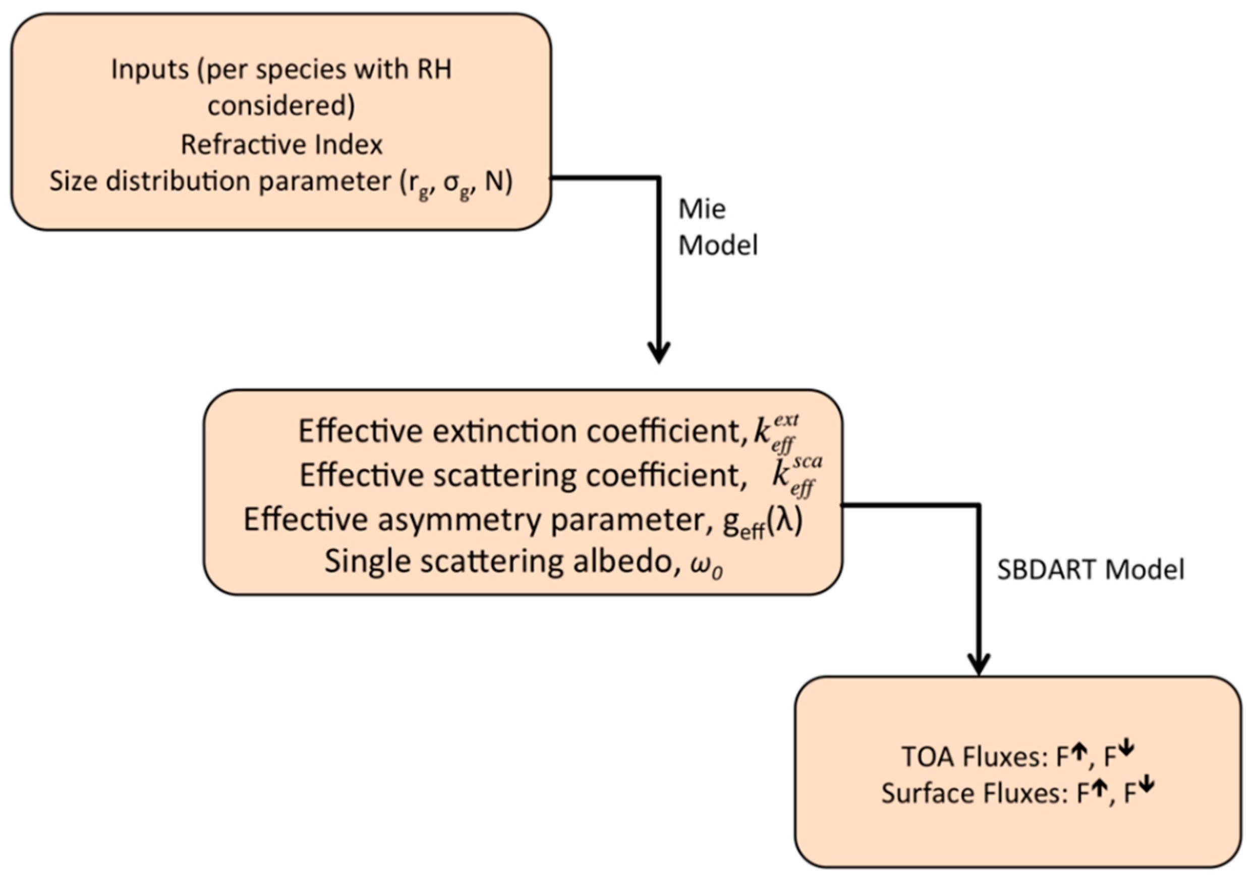
To access the radiative impacts of aerosols, many factors must be considered such as species, sources, concentrations, particle size distributions, atmospheric vertical structure, etc. We follow a similar methodology to both Benas et al. [6] and Menon et al. [7] in our modeling approach. In order to accurately represent regional south-eastern U. S. aerosols in both optical and radiative transfer models, we use information from both published literature and generic aerosol models that are frequently used in the radiative transfer modeling. Based on this information we constructed cases that are representative of mixtures of aerosol species and concentrations for season (winter or summer), constituents (urban or background) and physical process (biomass burning and suspended organic aerosol layer). For each case, the Mie optical modeling was performed to calculate the scattering and extinction coefficients, single scattering albedo (SSA or ω0) and asymmetry parameter (g) for wavelengths encompassing the shortwave portion of the electromagnetic spectrum (0.3–2.0 µm). The spectral aerosol optical depth (AOD) for each wavelength are calculated from computed extinction coefficients using satellite retrieved AOD at 550 nm [8] or aerosol concentrations and the aerosol layer depth. The spectral AOD, ω0, and g are used as input into the Santa Barbara Disort Atmospheric Radiative Transfer (SBDART) model to calculate TOA and surface radiative fluxes [9].
2.2. Optical Modeling Using Mie Theory
The Mie code requires input of the microphysical properties of each respective assemblage of aerosols. We consider four aerosol species that make up most of the measured PM2.5: sulfate, organics, black carbon (BC) and nitrates [10,11]. Size distributions in terms of the parameters R0 (the median radius) and σ (geometric standard deviation) of a log-normal function, and ρ (density) are taken from Optical Properties of Aerosols and Clouds (OPAC) [12]. To account for hygroscopic effects on sulfates and nitrates, R0 and the refractive indexes were calculated for each relative humidity (RH) of interest, e.g., RH of 75% for the winter cases and 90% for the summer cases.
To address seasonality, we compare the winter (W) with summer conditions (S) to create the four study cases: WB-Winter Background; WU-Winter Urban; SB-Summer Background; SU-Summer Urban. These cases were constructed based on the aerosol composition data from the EPA’s Air Quality System (http://www.epa.gov/airexplorer/). For sulfates we used ammoniated sulfates and for nitrates we used ammoniated nitrates based on the EPA data. Speciation concentrations were averaged for each season over all available data between years 2000–2009 (Figure 1).
For the aforementioned study cases we consider the species to be externally mixed in keeping with satellite retrieval algorithms; however, there is observational evidence to support internal mixtures of BC with other aerosol species. For addressing this type of internal mixture, we follow a methodology similar to Wang and Martin [13] and these cases will be denoted by WBi, WUi, SBi and SUi. We consider that all of the BC aerosols are covered by sulfate (~5% BC core by mass, with a sulfate shell), and that internally mixed BC/Sulfate aerosols form an external mixture with Organics and Nitrates (at appropriate RH). We calculate an effective refractive index based on the well-mixed sphere mixing rule [14] for a particle with the BC mass fraction presented in Table 2. These internally mixed cases should be considered representative of normal conditions during these seasons.
For the biomass burning case, PM2.5 speciation mass measurements from the 2007 GA wildfire from the Interagency Monitoring of Protected Visual Environments (IMPROVE) network are used [15]. Finally, for the aerosol layer aloft case, we use typical summertime aerosols for the first (lowest) layer, and the second layer is pure organics where measurements are provided by Hennigan et al. [16]. The Cloud-Aerosol Lidar and Infrared Pathfinder (CALIPSO) is used to identify the frequency of this occurrence in the region, see Section 2.3. The Mie model inputs and case names are summarized in Table 1 and Table 2. The parameter M* shown in Table 1 is the ratio of the mass concentration and the particle number concentration that was computed for each species to provide the conversion between the mass concentration and the particle number concentration.
The Mie optical model produces the normalized (per unit concentration) extinction, scattering and absorption coefficients, SSA, and asymmetry parameters for each species as a function of wavelength. The effective normalized coefficient of the mixture is:
where j represents each individual species, N is the total number concentration, and fj is the number fraction. The effective normalized scattering coefficient is given by similar expression so that the effective SSA (ω0) and the effective asymmetry parameter (g) are:
From the calculations of the effective extinction and scattering coefficients, the optical depth is simply the integration of the extinction coefficient for a layer in the atmosphere.
Using satellite derived AOD at 550 nm and layer depth (Δz) we can use Equation (4) to solve for the total number concentration per modeling case.
Multiplying by N gives the spectral AOD for each study case.
2.3. Radiative Transfer Modeling Using Santa Barbara Disort Atmospheric Radiative Transfer (SBDART)
The Mie optical model results are used as input to SBDART in terms of considering boundary layer aerosols that are representative of the south-eastern U.S. We modify the model to accept a user defined aerosol layer and the aerosol optical characteristics from the Mie modeling analysis. Since this region is covered year-round by evergreens, surface albedos do vary over seasons, but the magnitude of that variance is small, thus we use seasonal surface albedo values from the Moderate Resolution Imaging Spectroradiometer (MODIS) on board the Terra satellite [17,18]. We use regional spatially-averaged MODIS AOD to constrain the spectral AOD inputs from our Mie analysis into SBDART [18] to make the modeling cases more regionally specific than the default AOD within SBDART. As with our earlier work, we are using Collection 5 Level 2 aerosol over land MODIS products for AOD [19,20]. Since we are considering two seasons, we use the appropriate atmospheric profile (mid-latitude winter or mid-latitude summer). Additionally, we only consider shortwave (SW) fluxes, as the species considered here are not strongly reactive in the longer wavelengths. Table 2 summarizes the SBDART model inputs and Figure 2 presents a pictorial representation of the steps used for this modeling approach. We do not consider cloud fraction in this study, thus our analysis is representative of clear sky radiative effects.
2.4. Vertical Profile Analysis of CALIPSO Data
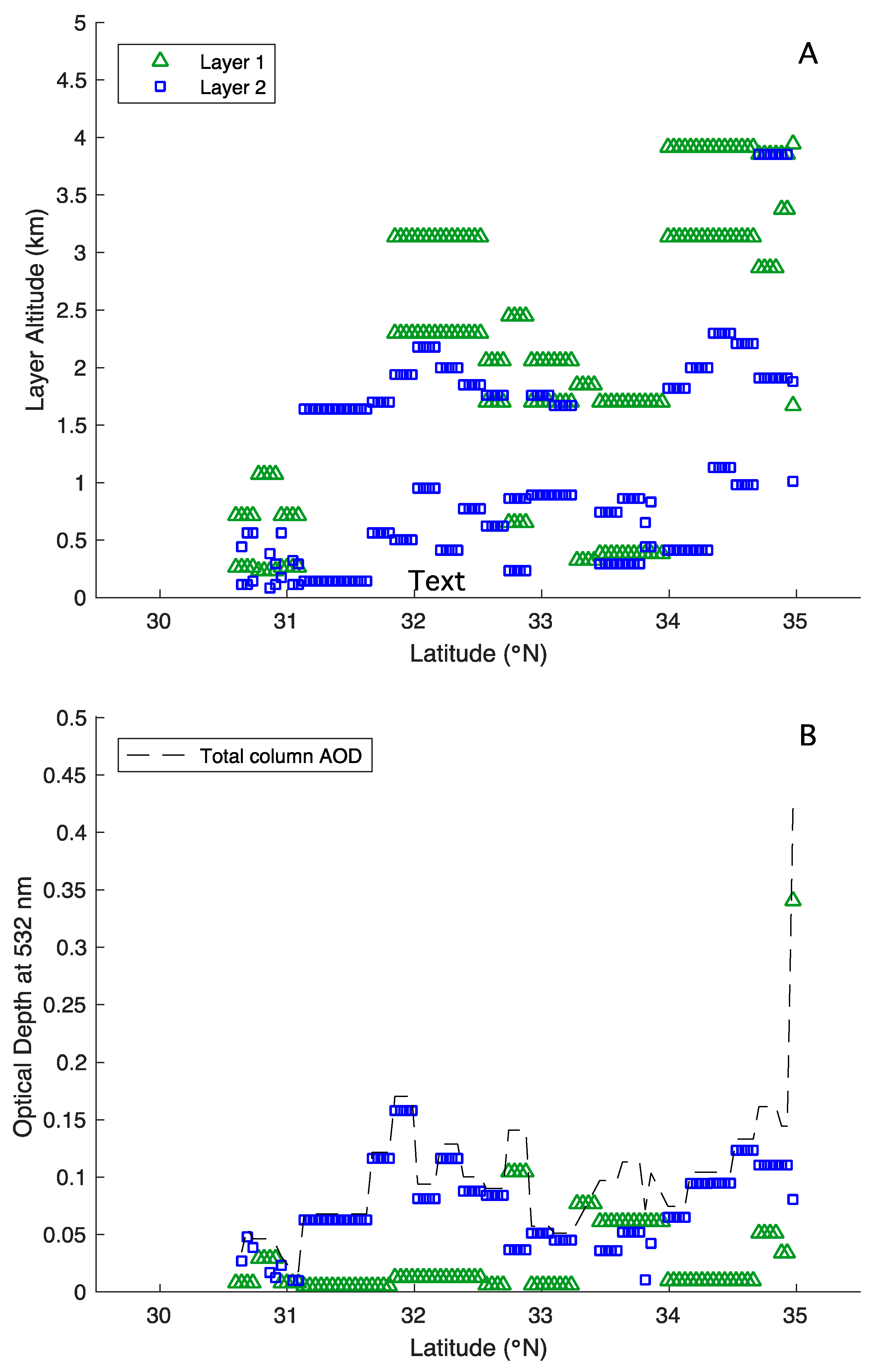
Different aerosol layer depths or mixing layer thicknesses are considered also. To determine the thickness of the layer (shown in Table 3), one-year of CALIPSO browse images are used to determine “average” heights of those layers. We looked at winter overpasses (December 2008–February 2009) and summer overpasses (June 2009–August 2009). We chose to use this year because we wanted a year where there were no problems with the laser and a year without any appreciable biomass burning in the region. We used CALIPSO Level 2 Aerosol Layer Data products Version 3.0 for this analysis [21]. Our analysis determined that during the winter, the aerosol layer was approximately 1km thick, and during the summer, the layer depth was about 2 km. Our analysis, which is summarized in Table 4 and Table 5, revealed that during the winter, there are a number of days where there are no aerosols present or if there were some aerosols, they were not in sufficiently high enough concentrations to have the significant backscattering at 532 nm. We also use this analysis to determine if there is a persistent organic aerosol layer aloft and, if there are two distinct layers, use the AOD and layer information from CALIPSO. Our analysis showed that there is no persistent aerosol layer aloft over this region, which is a tenet of the hypothesis from Goldstein et al. [22]. Goldstein et al., offer different definitions of what “aloft” means, but they do not provide a clear single answer. Further casting doubt on this hypothesis is work by Heald et al. [23], which concludes that data from 17 field experiments do not substantiate elevated secondary organic aerosols (SOA) in the mid-troposphere where it is often predicted to be by models. It is possible that due to some of CALIPSO’s limitations in the PBL and being unable to discriminate between SOA and other aerosols, that there are aerosols present aloft so, we do consider a case where an aerosol layer consisting of organics is aloft from a lower layer of typical summertime aerosols (SALA case). Our analysis revealed one date (14 August 2009) where there were two distinct aerosol layers, see Figure 3. During this nighttime overpass, the lowest layer (0–2 km) is identified as primarily polluted continental (lidar ratio of 70) with some areas identified as polluted dust (lidar ratio of 55) and has an AOD of 0.11, and the upper layer (2.5–3.5 km) is primarily clean continental (lidar ration of 35) with an AOD of 0.03. Although the CALIPSO’s problem of misidentifying some polluted aerosols as polluted dust is still a minor issue, the majority of the aerosol typing was correct. The overall accuracy of the CALIPSO AOD is based on the pre-determined lidar ratio; thus if the aerosols are incorrectly identified the lidar ratio used to estimate AOD could result in errors in the accuracy of CALIPSO AOD [24]. While the CALIPSO-derived AOD values are slightly on the low side compared to typical MODIS AOD in the region, we hypothesize that problems with CALIPSO selecting the correct lidar ratio could be a possible reason why CALIPSO AOD is biased low against MODIS AOD [25]. This current research does not explore the accuracy of CALIPSO AOD in this region, as we primarily use CALIPSO data for providing a basis a modeling case. We use our unpublished results from the biomass burning case studies to determine that for most of the biomass burning events there is only one layer of aerosols that is approximately 2 km thick (SBB case), and this value has good agreement with published analysis from a recent wildfire in Georgia [15] from 2007, which found biomass burning aerosols in a layer approximately 2–3 km thick, see Table 3 for the SBDART modeling cases.
3. Results
3.1. Analysis of Optical Modeling Results of South-Eastern U.S. Aerosols
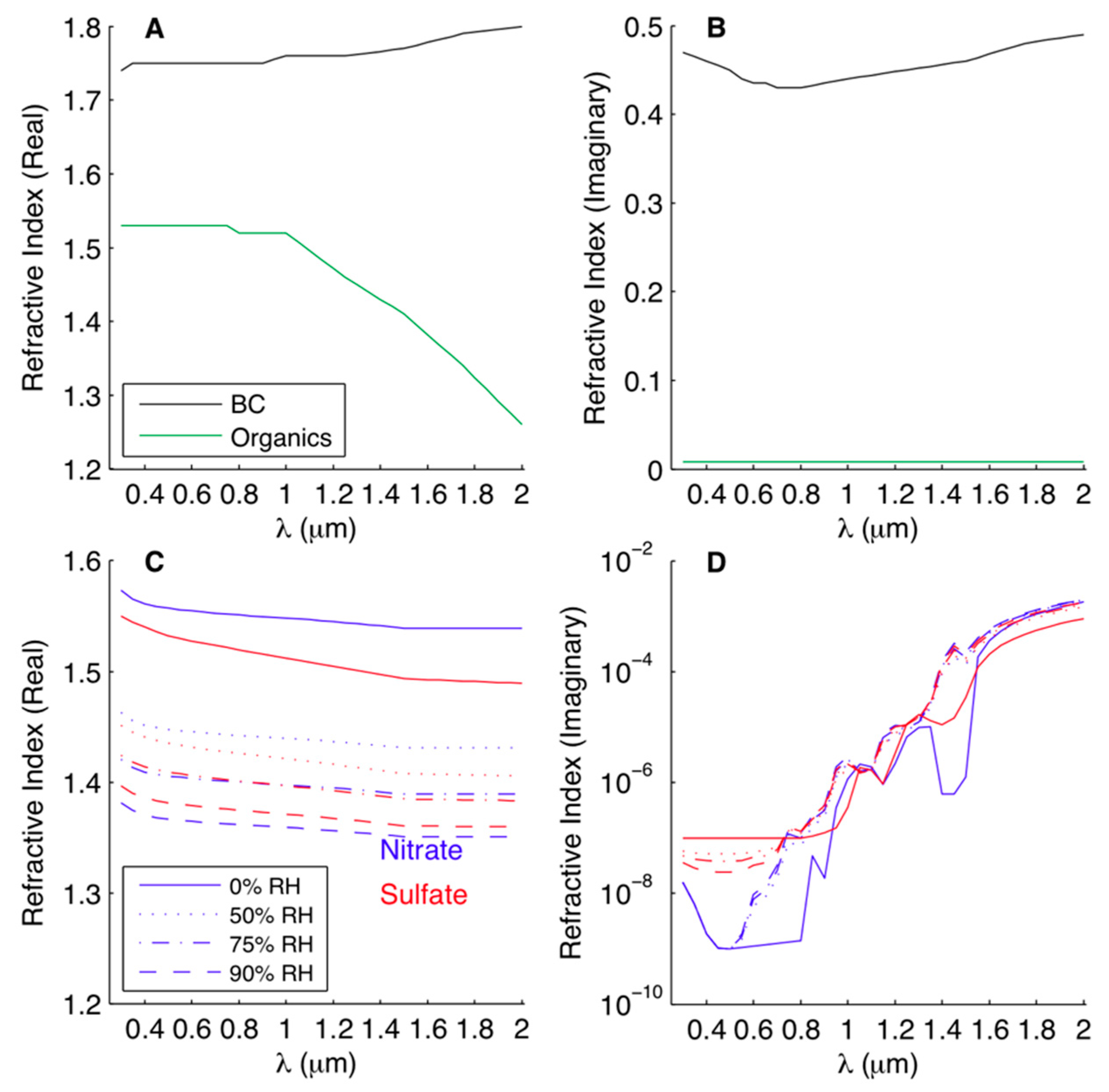
Figure 4 shows the refractive indexes for sulfates and nitrates computed at multiple RH of 0% (dry salt), 50%, 75% (winter) and 90% (summer). As expected the only species with significant absorption as measured by the imaginary part of the refractive index is BC, Organics and the BC/Sulfate internal mixture. The other species can be called essentially light scattering.
In the shorter wavelengths, sulfates and nitrates have different behaviors in their absorption spectra, but as wavelengths increase the behavior of both becomes similar. For nitrates, the dry salt has the strongest absorption relative to the other nitrate measurements at increasing RH. Sulfate behaves opposite of nitrate, where increases in RH lead to slightly more absorption. In the scattering spectra for sulfates and nitrates, the dry salts are the most scattering, while the uptake of water leads to decreases in scattering.
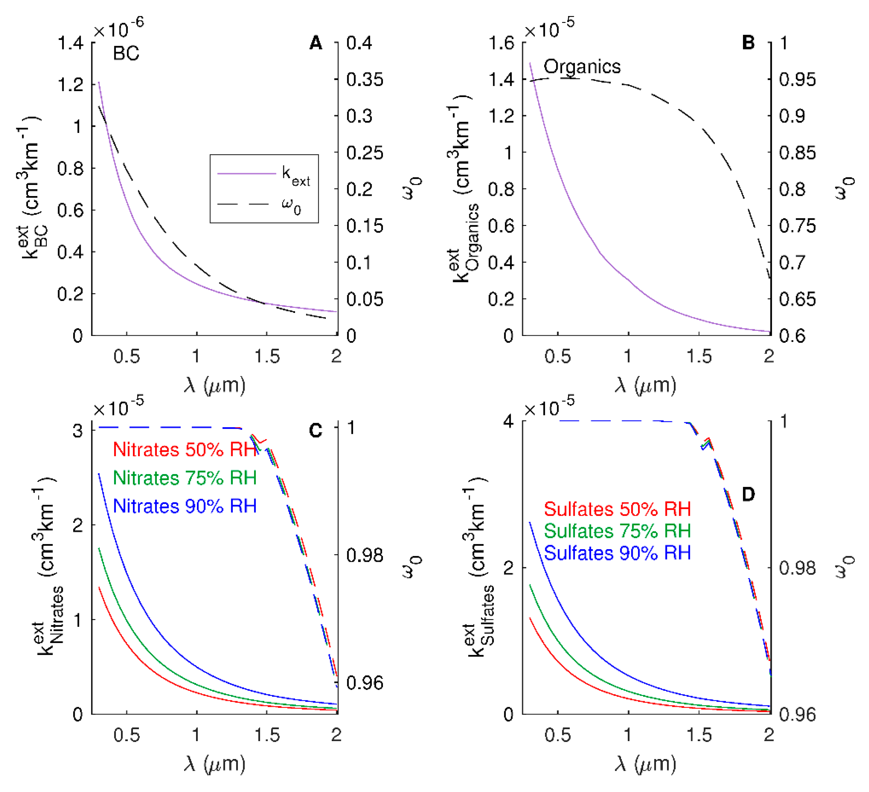
The Mie optical model requires each species be modeled individually and the external mixture of aerosols is done afterward for each study case. Figure 5 shows the normalized (per unit number concentration) extinction coefficient and ω0 for each species.
The behaviors of the extinction and ω0 curves are similar for sulfates and nitrates. The single scattering albedo (ω0) provides additional information that can be used in interpreting the optical depth. The single scattering albedo is defined as the ratio between the scattering coefficient and the extinction coefficient. A high value of ω0 implies that scattering is more dominant, vice versa small values imply absorption is more dominant. BC has the smallest extinction, but has the lowest ω0, while ω0 for organics falls in between the other species.
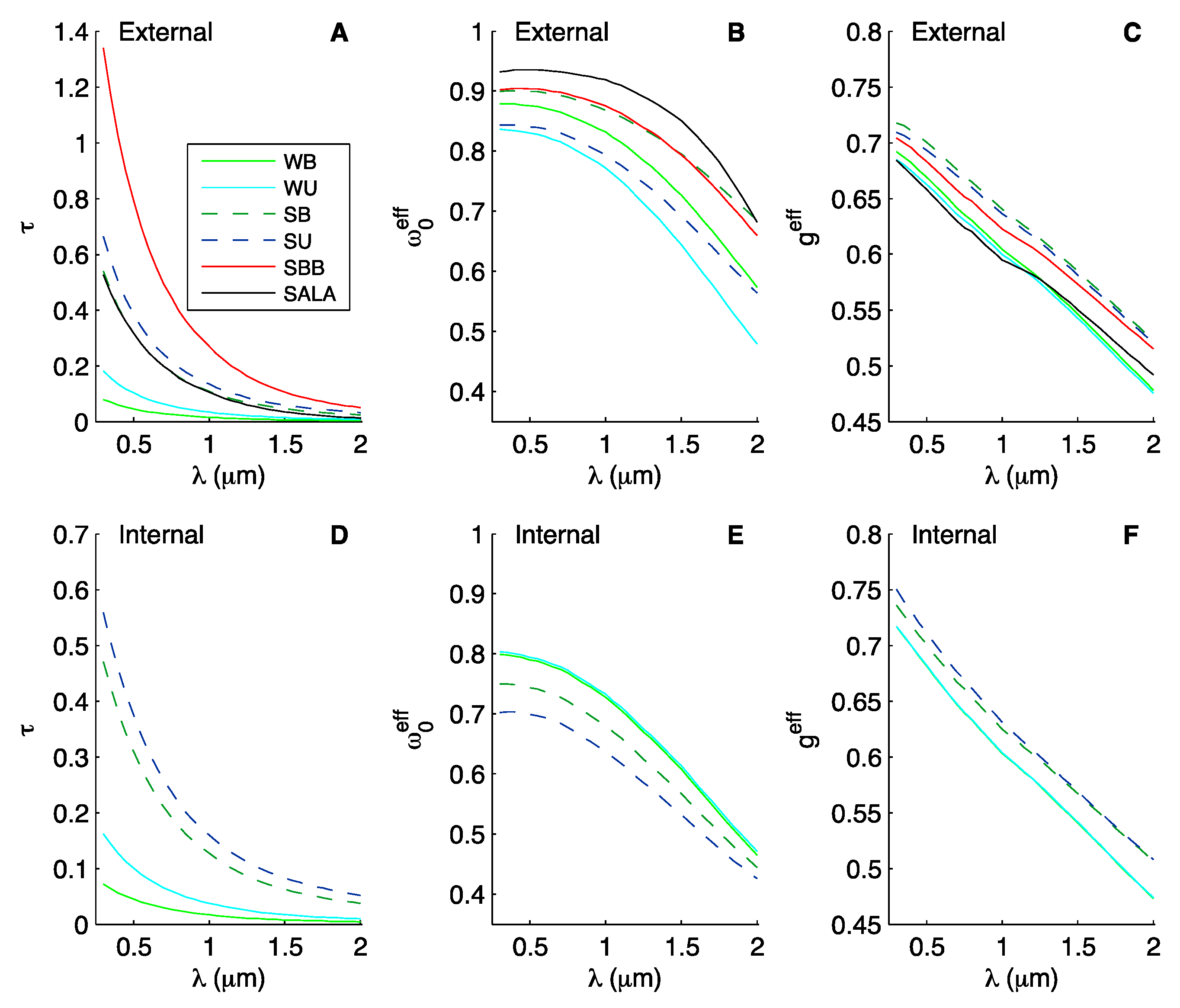
The outputs from the optical model are normalized properties and must be multiplied by the number concentrations per species for each case to obtain effective layer properties. Earlier MODIS AOD analyses from Alston et al. [18] were used to determine a representative AOD at 550 nm for each study case. Through Equations (1)–(5) we can then calculate the total number concentration, which can then be multiplied by the effective normalized extinction coefficient to determine the spectral AOD for 0.2–2.0 µm. The spectral AOD (or τ) are shown in Figure 6. The addition of a layer of organics above typical summer background conditions causes increased extinction. The biomass burning case (SBB) had the highest spectral AOD with values around 1.2 in the visible range, and the winter cases have the lowest AOD with values below 0.2. Though these effective properties are tuned to match satellite observed AOD, it would be useful to compare the spectral properties with those from Aerosol Robotic Network (AERONET); however, there are no AERONET stations in our region of interest. The effective asymmetry parameter (g) behaves similarly for all of the cases, with small differences between the cases (Figure 6). In fact, for the winter and summer cases, they are virtually the same. The urban cases have the lowest effective ω0, followed by the background winter conditions. The cases with the highest ω0 are the winter cases and the aerosol layer aloft (SALA). These effective ω0 agree well with published literature data that show that scattering aerosols dominate this region [11,23,26,27]. Also, these ω0 agree well with satellite estimates of ω0 from Multi-angle Imaging SpectroRadiometer (MISR), see Figure 6, though for the internal mixture SSA values are lower with ranges in the visible spectrum around 0.7–0.8. Wang and Martin [13] found a similar result in SSA relating to external mixtures and internal mixtures.
3.2. Analysis of Modeled Radiative Forcing
In Alston and Sokolik [5] we performed an estimate of TOA radiative forcing using the first order approximation where we used time-series of the surface albedo, cloud fraction and satellite AOD from both MODIS and MISR. However, that approximation is only applicable to TOA and cannot be used to determine the extent of surface forcing, not only for typical conditions (e.g., WB, SB) but for special cases such as biomass burning or deciphering the presence of an organic aerosol layer aloft. Thus, we use the SBDART radiative model to perform an assessment of TOA and surface forcing for our study cases (see Table 1 and Table 2).
We define the radiative forcing as the difference in fluxes between clean atmosphere (refers to the model run without any aerosols) and aerosols (refers to the model run with aerosols as specified in Table 3):
In the above equations, the direction of the net fluxes are represented by: ↑ = upward flux and ↓ = downward flux. Using this convention negative values of ΔF are indicative of net aerosol cooling, and positive values are indicative of net aerosol warming.
Comparisons between the different cases are dependent upon aerosol speciation, concentration and RH, so we define the radiative forcing efficiency (RFE) as:
RFE is a useful metric because it makes for easier comparisons of forcing despite changes in the aerosol type. We use AOD at 550 nm from MODIS (see Table 3). RFE is calculated for both the TOA and surface forcings. The units for RFE are Wm−2 τ−1.
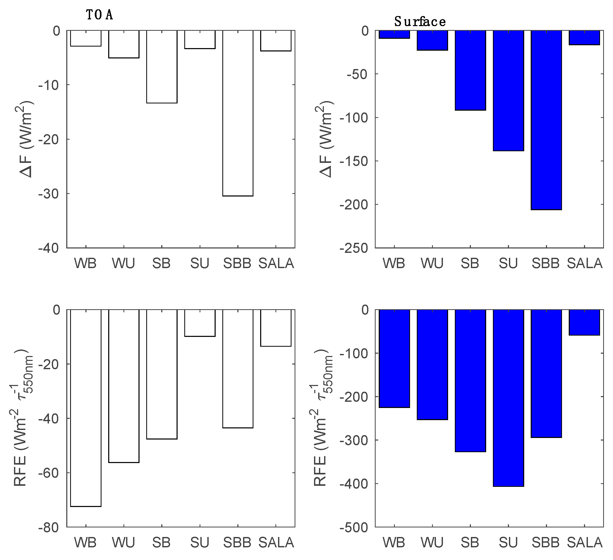
We show modeled TOA and surface forcing and RFE for the study cases in Figure 7. All the aerosol mixtures from the study cases result in negative TOA and surface forcing. The special summer cases SBB (biomass burning) and SALA (organic aerosol layer aloft) have the largest forcings in absolute terms. In fact, SBB produces three times more TOA forcing than the other cases. During the winter, modeled TOA forcing is −2.8 and −5 W/m2 for the WB and WU cases, and these values generally agree with the estimated forcing from Alston and Sokolik [5]. The modeled summer TOA forcings (SB = −13.3 W/m2) also generally agree well with earlier estimates. Interestingly, the study case that is representative of the Atlanta metropolitan area has less forcing (SU = −3.3 W/m2) in absolute terms compared with background conditions. A possible explanation of this difference could be ascribed to the differences in AOD between the urban (τ = 0.34) and background (τ = 0.28) cases. All of the aerosol cases result in negative surface forcing (cooling), a component that has not been explored previously. The SBB case had the largest degree of the surface cooling, with the next highest being the summer cases. All of these estimates of the forcing presented in this research are significantly higher than those predicted by the Intergovernmental Panel on Climate Change (IPCC) (1.5 W/m2) [28] although they consider global TOA forcing (~ 1.5 W/m2) as opposed to our regional study.
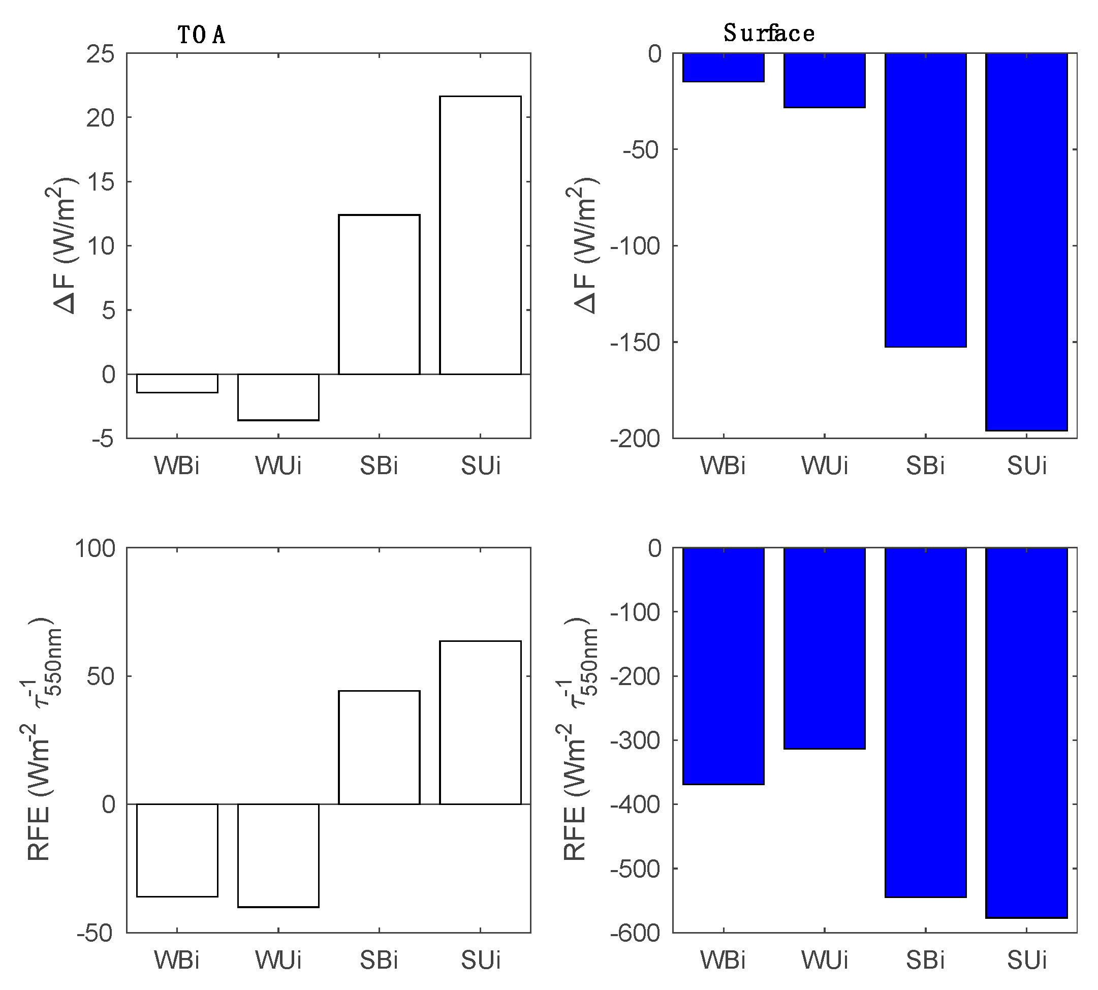
Comparisons of RFE of the study cases reveals that Figure 7 also shows that the externally mixed cases have less variability on the case to case basis for the winter cases in terms of RFE. We find that the urban cases have higher RFE than background conditions at the surface, yet WB, WU, SB have RFE that vary between −40 to −70 Wm−2 τ−1. The winter cases appear to be more efficient at forcing at the TOA. The SU case is unexpected in terms of comparing its RFE from the surface with the TOA. The SU case has the lowest RFE for TOA forcing of −9.8 Wm−2 τ−1, yet has the largest RFE for surface forcing of −406.7 Wm−2 τ−1. As Figure 7 shows the SU case has slightly more BC than the SB case, it is likely this increase in BC lead to a more pronounced warming. This suggests that the region experiences TOA cooling year around as opposed to just the summer as is implied in Goldstein et al. [22]. Also our modeled TOA forcing (WB, SB, and SALA) agrees better with Goldstein et al. than our estimated TOA forcing calculated earlier Alston and Sokolik [5]. This could be because we are using a seasonally averaged AOD value from MODIS, instead of a continuously varying AOD time series. Interestingly, the biomass burning case (SBB) has similar forcing efficiencies (−44 Wm−2 τ−1) to that of summer background conditions (−47.6 Wm−2 τ−1). This has an interesting implication for those situations where biomass burning aerosols are located aloft, our results suggest that in those cases the surface may experience increased surface level forcing. Lastly, we present study cases using the interally mixed cases (WBi, WUi, SBi, and SUi) in Figure 8. We wanted to present an analysis that is based on observational studies where BC has been internally mixed with sulfate. An interesting observation is that for the interally mixed cases, the net forcing at the surface is similar to those cases of externally mixed aerosols, but the net forcing at the TOA results in appreciabily different values for the summer cases. We know that BC is has higher forcing at the TOA than surface, at shorter wavelengths, which is what shown in these results. Given that the number concentrations of the internally mixed BC core sulfate shell aerosols are higher in the summer, it would be expected to see net warming at the TOA for these cases. It follows that the RFE for the summer internally mixed cases is not only opposite in sign (warming instead of cooling) and larger in magnitude compared to the externally mixed cases (RFE SU = −48 Wm−2 τ−1 vs. RFE SUi = 60 Wm−2 τ−1).
4. Discussion
It is important to provide context of these results to the greater body of research in the topical area and geographical area. For instance, Carrico et al. [3] found forcing to be approximately −11 W/m2 during the 1999 Atlanta Supersite study. This estimate was derived from a summertime field study in downtown Atlanta, GA which measured the optical properties of PM2.5 (particulate matter with aerodynamic radii <2.5 μm). Our analysis shows good agreement with the SB (summer background) case with the findings of Carrico et al. [3], while our results underperform for the urban conditions that could be attributed to the initialization conditions of our aerosol mixtures.
Mao et al. [4] conducted a thorough examination of model based research for the south-eastern U.S. as a high level overview of the literature to provide pertinent context for the SAS. This research highlights an interesting aspect of climate in the region, namely that of the warming hole due to aerosol effects. There are dueling perspectives on climate and radiation impacts of aerosol effects from both natural and anthropogenic sources [29,30,31]. The research here does not necessarily seek to answer this debate, however, the hypothesis of Y. Lee et al. [32] does offer intriguing insights into a future climate scenario where air pollution control policies may have in had an impact. Carlton et al. [33] posit that biogenic sources of SOA can be regulated similar to air pollution, which raises interesting future considerations for policy makers. Future research in this area could focus upon exploring the linkages between reduced forcing (less negative) and potential derived health benefits for this region. Additionally, while this research focuses on clear sky conditions, it would be intriguing to perform this same analysis by taking cloud effects into account by estimating all-sky conditions.
5. Conclusions
We presented the results on modeling radiative forcing at the TOA and surface through the use of optical models and 1-D radiative transfer model (SBDART). We used representative microphysical properties to calculate optical properties of BC, organics, sulfates and nitrates as external mixtures. We also considered study cases where BC was coated with sulfate for an internal mixture. We used results from the Mie optical model of the effective aerosol layer properties to predict surface and TOA forcing using SBDART. We found that all of externally mixed aerosol cases considered resulted in negative TOA radiative forcing. The radiative forcing efficiency at the TOA varied from −9 to −72 Wm−2 τ−1, while RFE at the surface varied from −50 to −410 Wm−2 τ−1. Interestingly the RFE at the TOA was similar for the winter cases, and the modeled TOA forcing was more similar to the estimated forcing calculated by Goldstein et al. [22]. The RFE of biomass burning both at the TOA and surface were similar to the RFE of summer background aerosol. This result has direct implications for biomass burning radiative effects in this region especially in the context of a potentially warming climate. The interpretation of the internally mixed cases yield interesting considerations for future studies. While satellite retrievals consider externally mixed aerosols, our results show that when internally mixed aerosols are considered, not only does the magnitude of the forcing increase slightly but it also results in a warming at the TOA, compared to externally mixed cases representing the TOA (RFE SB = −48 Wm−2 τ−1 vs. RFE SBi = 48 Wm−2 τ−1 and RFE SU = −10 Wm−2 τ−1 vs. RFE SUi = 60 Wm−2 τ−1). This has implications in regions where this type of mixture is more common, and could impact satellite retrieval values of aerosol properties.
Author Contributions
Conceptualization, E.J.A. and I.N.S.; Methodology, E.J.A. and I.N.S..; Formal Analysis, E.J.A..; Investigation, E.J.A..; Resources, E.J.A. and I.N.S Writing-Original Draft Preparation, E.J.A.; Writing-Review and Editing, E.J.A. and I.N.S..; Visualization, E.J.A.
Funding
For E.J.A.—This research was funded by the National Aeronautics and Space Administration (NASA) Office of Education National Space Grant Program Office. For I.N.S.—This research was funded by NASA Atmospheric Radiation Program and the National Science Foundation.
Acknowledgments
The authors would like to thank the NASA Science Mission Directorate and the NASA Office of Education for their support.
Conflicts of Interest
The authors declare no conflict of interest.
References
- Carlton, A.G.; de Gouw, J.; Jimenez, J.L.; Ambrose, J.L.; Attwood, A.R.; Brown, S.; Baker, K.R.; Brock, C.; Cohen, R.C.; Edgerton, S.; et al. Synthesis of the southeast atmosphere studies: Investigating fundamental atmospheric chemistry questions. Bull. Am. Meteorol. Soc. 2018, 99, 547–567. [Google Scholar] [CrossRef]
- Edgerton, E.S.; Hartsell, B.E.; Saylor, R.D.; Jansen, J.J.; Hansen, D.A.; Hidy, G.M. The southeastern aerosol research and characterization study, part 3: Continuous measurements of fine particulate matter mass and composition. J. Air Waste Manag. 2006, 56, 1325–1341. [Google Scholar] [CrossRef]
- Carrico, C.M.; Bergin, M.H.; Xu, J.; Baumann, K.; Maring, H. Urban aerosol radiative properties: Measurements during the 1999 Atlanta Supersite Experiment. J. Geophys. Res. 2003, 108. [Google Scholar] [CrossRef] [Green Version]
- Mao, J.; Carlton, A.; Cohen, R.C.; Brune, W.H.; Brown, S.S.; Wolfe, G.M.; Jimenez, J.L.; Pye, H.O.T.; Lee Ng, N.; Xu, L.; et al. Southeast atmosphere studies: Learning from model-observation syntheses. Atmos. Chem Phys. 2018, 18, 2615–2651. [Google Scholar] [CrossRef] [PubMed]
- Alston, E.J.; Sokolik, I.N. A first-order assessment of direct aerosol radiative effect in the southeastern U.S. Using over a decade long multisatellite data record. Air Soil Water Res. 2016, 9. [Google Scholar] [CrossRef]
- Benas, N.; Hatzianastassiou, N.; Matsoukas, C.; Fotiadi, A.; Mihalopoulos, N.; Vardavas, I. Aerosol shortwave direct radiative effect and forcing based on MODIS Level 2 data in the Eastern Mediterranean (Crete). Atmos. Chem. Phys. 2011, 11, 12647–12662. [Google Scholar] [CrossRef] [Green Version]
- Menon, S.; Akbari, H.; Mahanama, S.; Sednev, I.; Levinson, R. Radiative forcing and temperature response to changes in urban albedos and associated CO2 offsets. Environ. Res. Lett. 2010, 5, 014005. [Google Scholar] [CrossRef]
- Levy, R.C.; Mattoo, S.; Munchak, L.A.; Remer, L.A.; Sayer, A.M.; Patadia, F.; Hsu, N.C. The collection 6 modis aerosol products over land and ocean. Atmos. Meas. Tech. 2013, 6, 2989–3034. [Google Scholar] [CrossRef]
- Ricchiazzi, P.; Yang, S.; Gautier, C.; Sowle, D. SBDART: A research and teaching software tool for plane-parallel radiative transfer in the Earth’s atmosphere. Bull. Am. Meteorol. Soc. 1998, 79, 2101–2114. [Google Scholar] [CrossRef]
- Butler, A.J.; Andrew, M.S.; Russell, A.G. Daily sampling of PM2.5 in Atlanta: Results of the first year of the assessment of spatial aerosol composition in Atlanta study. J. Geophys. Res. 2003, 108. [Google Scholar] [CrossRef]
- Edgerton, E.S.; Hartsell, B.E.; Saylor, R.D.; Jansen, J.J.; Hansen, D.A.; Hidy, G.M. The southeastern aerosol research and characterization study: Part II. Filter-based measurements of fine and coarse particulate matter mass and composition. J. Air Waste Manag. 2005, 55, 1527–1542. [Google Scholar] [CrossRef]
- Hess, M.; Koepke, P.; Schult, I. Optical properties of aerosols and clouds: The software package OPAC. Bull. Am. Meteorol. Soc. 1998, 79, 831–844. [Google Scholar] [CrossRef]
- Wang, J.; Martin, S.T. Satellite characterization of urban aerosols: Importance of including hygroscopicity and mixing state in the retrieval algorithms. J. Geophys. Res. 2007, 112, D17203. [Google Scholar] [CrossRef]
- Lesins, G.; Chylek, P.; Lohmann, U. A study of internal and external mixing scenarios and its effect on aerosol optical properties and direct radiative forcing. J. Geophys. Res. 2002, 107, 4094. [Google Scholar] [CrossRef]
- Christopher, S.A.; Gupta, P.; Nair, U.; Jones, T.J.; Kondragunta, S.; Wu, Y.L.; Hand, J.L.; Zhang, X. Satellite remote sensing and mesoscale modeling of the 2007 Georgia/Florida fires. IEEE J. Sel. Top. App. Rem. Sens. 2009, 2, 163–175. [Google Scholar]
- Hennigan, C.J.; Bergin, M.H.; Russell, A.G.; Nenes, A.; Weber, R.J. Gas/particle partitioning of water-soluble organic aerosol in Atlanta. Atmos. Chem. Phys. 2009, 9, 3613–3628. [Google Scholar] [CrossRef] [Green Version]
- Schaaf, C.B.; Gao, F.; Strahler, A.H.; Lucht, W.; Li, X.; Tsang, T.; Strugnell, N.C.; Zhang, X.; Jin, Y.; Muller, J.-P.; et al. First operational BRDF, albedo nadir reflectance products from MODIS. Remote Sens. Environ. 2002, 83, 135–148. [Google Scholar] [CrossRef] [Green Version]
- Alston, E.J.; Sokolik, I.N.; Kalashnikova, O.V. Characterization of atmospheric aerosol in the US southeast from ground- and space-based measurements over the past decade. Atmos. Meas. Tech. 2012, 5, 1667–1682. [Google Scholar] [CrossRef]
- Levy, R.C.; Remer, L.A.; Kleidman, R.G.; Mattoo, S.; Ichoku, C.; Kahn, R.; Eck, T.F. Global evaluation of the collection 5 MODIS dark-target aerosol products over land. Atmos. Chem. Phys. 2010, 10, 10399–10420. [Google Scholar] [CrossRef] [Green Version]
- Levy, R.C.; Remer, L.A.; Mattoo, S.; Vermote, E.F.; Kaufman, Y.J. Second-generation operational algorithm: Retrieval of aerosol properties over land from inversion of moderate resolution imaging spectroradiometer spectral reflectance. J. Geophys. Res. 2007, 112, D13211. [Google Scholar] [CrossRef]
- Vaughan, M.A.; Powell, K.A.; Kuehn, R.E.; Young, S.A.; Winker, D.M.; Hostetler, C.A.; Hunt, W.H.; Liu, Z.; McGill, M.J.; Getzewich, B.J. Fully automated detection of cloud and aerosol layers in the calipso lidar measurements. J. Atmos. Ocean. Techol. 2009, 26, 2034–2050. [Google Scholar] [CrossRef]
- Goldstein, A.H.; Koven, C.D.; Heald, C.L.; Fung, I.Y. Biogenic carbon and anthropogenic pollutants combine to form a cooling haze over the southeastern United States. Proc. Natl. Acad. Sci. USA 2009, 106, 8835–8840. [Google Scholar] [CrossRef] [PubMed] [Green Version]
- Heald, C.L.; Coe, H.; Jimenez, J.L.; Weber, R.J.; Bahreini, R.; Middlebrook, A.M.; Russell, L.M.; Jolleys, M.; Fu, T.M.; Allan, J.D.; et al. Exploring the vertical profile of atmospheric organic aerosol: Comparing 17 aircraft field campaigns with a global model. Atmos. Chem. Phys. Discuss. 2011, 11, 25371–25425. [Google Scholar] [CrossRef]
- Omar, A.H.; Winker, D.M.; Kittaka, C.; Vaughan, M.A.; Liu, Z.; Hu, Y.; Trepte, C.R.; Rogers, R.R.; Ferrare, R.A.; Lee, K.P.; et al. The CALIPSO automated aerosol classification and lidar ratio selection algorithm. J. Atmos. Ocean. Techol. 2009, 26, 1994–2014. [Google Scholar] [CrossRef]
- Kittaka, C.; Winker, D.M.; Vaughan, M.A.; Omar, A.; Remer, L.A. Intercomparison of column aerosol optical depths from CALIPSO and MODIS-Aqua. Atmos. Meas. Tech. 2011, 4, 131–141. [Google Scholar] [CrossRef] [Green Version]
- Blanchard, C.L.; Hidy, G.M.; Tanenbaum, S.; Edgerton, E.S. NMOC, ozone, and organic aerosol in the southeastern United States, 1999–2007: 3. Origins of organic aerosol in Atlanta, Georgia, and surrounding areas. Atmos. Environ. 2011, 45, 1291–1302. [Google Scholar] [CrossRef]
- Tombach, I.; Brewer, P. Natural background visibility and regional haze goals in the southeastern United States. J. Air Waste Manag. 2005, 55, 1600–1620. [Google Scholar] [CrossRef]
- Forster, P.; Ramaswamy, V.; Artaxo, P.; Berntsen, T.; Betts, R.; Fahey, D.W.; Haywood, J.; Lean, J.; Lowe, D.C.; Myhre, G.; et al. Changes in atmospheric constituents and in radiative forcing. In Climate Change 2007: The Physical Science Basis. Contribution of Working Group I to the Fourth Assessment Report of the Intergovernmental Panel on Climate Change; Solomon, S., Qin, D., Manning, M., Chen, Z., Marquis, M., Averyt, K.B., Tignor, M., Miller, H.L., Eds.; Cambridge University Press: Cambridge, UK; New York, NY, USA, 2007. [Google Scholar]
- Tosca, M.; Campbell, J.; Garay, M.; Lolli, S.; Seidel, F.; Marquis, J.; Kalashnikova, O. Attributing accelerated summertime warming in the southeast United States to recent reductions in aerosol burden: Indications from vertically-resolved observations. Remote Sens. 2017, 9, 674. [Google Scholar] [CrossRef]
- Cusworth, D.H.; Mickley, L.J.; Leibensperger, E.M.; Iacono, M.J. Aerosol trends as a potential driver of regional climate in the central united states: Evidence from observations. Atmos. Chem. Phys. 2017, 17, 13559–13572. [Google Scholar] [CrossRef]
- Yu, S.; Alapaty, K.; Mathur, R.; Pleim, J.; Zhang, Y.; Nolte, C.; Eder, B.; Foley, K.; Nagashima, T. Attribution of the United States “warming hole”: Aerosol indirect effect and precipitable water vapor. Sci. Rep. 2014, 4, 6929. [Google Scholar] [CrossRef] [PubMed]
- Lee, Y.; Shindell, D.T.; Faluvegi, G.; Pinder, R.W. Potential impact of a us climate policy and air quality regulations on future air quality and climate change. Atmos. Chem. Phys. 2016, 16, 5323–5342. [Google Scholar] [CrossRef]
- Carlton, A.G.; Pinder, R.W.; Bhave, P.V.; Pouliot, G.A. To what extent can biogenic SOA be controlled? Environ. Sci. Technol. 2010, 44, 3376–3380. [Google Scholar] [CrossRef] [PubMed]
Figure 1.
Mass fractions of BC (black carbon), organics, sulfates and nitrates for the modeling cases (see also Table 1).
Figure 1.
Mass fractions of BC (black carbon), organics, sulfates and nitrates for the modeling cases (see also Table 1).

Figure 2.
Schematic of general modeling approach.

Figure 3.
(A) CALIPSO layer base and top and (B) CALIPSO layer AOD for August 14, 2009 with an overpass time of 4:37 a.m. EDT. Longitudes vary from approximately 83.8° W to 85° W.
Figure 3.
(A) CALIPSO layer base and top and (B) CALIPSO layer AOD for August 14, 2009 with an overpass time of 4:37 a.m. EDT. Longitudes vary from approximately 83.8° W to 85° W.

Figure 4.
Refractive indices for Black Carbon and Organics (A) real and (B) imaginary. Refractive indices for Nitrate and Sulfate (C) real and (D) imaginary. Refractive indices are calculated over wavelengths 0.3–2.0 µm. Nitrates and sulfates are shown for 0%, 50%, 75% and 90% RH.
Figure 4.
Refractive indices for Black Carbon and Organics (A) real and (B) imaginary. Refractive indices for Nitrate and Sulfate (C) real and (D) imaginary. Refractive indices are calculated over wavelengths 0.3–2.0 µm. Nitrates and sulfates are shown for 0%, 50%, 75% and 90% RH.

Figure 5.
Extinction coefficient () and ω0 for BC (A); organics (B); nitrates (C); sulfates (D). Nitrates and sulfates are shown at RH of 50%, 75% and 90%.
Figure 5.
Extinction coefficient () and ω0 for BC (A); organics (B); nitrates (C); sulfates (D). Nitrates and sulfates are shown at RH of 50%, 75% and 90%.

Figure 6.
Effective AOD (τ), ω0 for wavelengths 0.3–2.0 µm, and asymmetry parameter (g) for each study case (A–C) externally mixed aerosols and (D–F) internally mixed aerosols.
Figure 6.
Effective AOD (τ), ω0 for wavelengths 0.3–2.0 µm, and asymmetry parameter (g) for each study case (A–C) externally mixed aerosols and (D–F) internally mixed aerosols.

Figure 7.
Modeled radiative forcing (top) and radiative forcing efficiency (RFE) (bottom) at the top-of-atmosphere (TOA) (white bars) and surface (blue bars) for the study cases.
Figure 7.
Modeled radiative forcing (top) and radiative forcing efficiency (RFE) (bottom) at the top-of-atmosphere (TOA) (white bars) and surface (blue bars) for the study cases.

Figure 8.
Modeled radiative forcing (top) and RFE (bottom) at the TOA (white bars) and surface (blue bars) for the study cases of internally mixed aerosols.
Figure 8.
Modeled radiative forcing (top) and RFE (bottom) at the TOA (white bars) and surface (blue bars) for the study cases of internally mixed aerosols.


Table 1.
Study case names and microphysical properties used in the optical modeling of externally mixed aerosols species.
Table 1.
Study case names and microphysical properties used in the optical modeling of externally mixed aerosols species.
| Model Cases | ||||||||
|---|---|---|---|---|---|---|---|---|
| WB (Winter Background) | WU (Winter Urban) | |||||||
| Microphysical Properties | BC (Black Carbon) | Organics | Sulfates 75% | Nitrates 75% | BC (Black Carbon) | Organics | Sulfates 75% | Nitrates 75% |
| R0 | 0.01188 | 0.0296 | 0.0296 | 0.0296 | 0.0118 | 0.0296 | 0.0296 | 0.0296 |
| ln σ | 0.6931 | 0.8065 | 0.8065 | 0.8605 | 0.6931 | 0.8065 | 0.8065 | 0.8065 |
| Density (ρ) (g/cm3) | 1.00 | 2.00 | 1.30 | 1.30 | 1.00 | 2.00 | 1.30 | 1.30 |
| M* (µg/m3)/cm−3 | 5.98 × 10⁻⁵ | 2.81 × 10⁻⁵ | 1.83 × 10⁻³ | 1.83 × 10⁻³ | 5.98 × 10⁻⁵ | 2.81 × 10⁻³ | 1.83 × 10⁻³ | 1.83 × 10⁻³ |
| Mass Fraction | 0.0636 | 0.4475 | 0.3359 | 0.1530 | 0.0933 | 0.4443 | 0.2976 | 0.1648 |
| Number Fraction | 0.7139 | 0.1067 | 0.1232 | 0.0561 | 0.7915 | 0.0801 | 0.0826 | 0.0457 |
| SB (Summer Background) | SU (Summer Urban) | |||||||
| Microphysical Properties | BC (Black Carbon) | Organics | Sulfates 90% | Nitrates 90% | BC (Black Carbon) | Organics | Sulfates 90% | Nitrates 90% |
| R0 | 0.0118 | 0.0348 | 0.0348 | 0.0348 | 0.0118 | 0.0348 | 0.0348 | 0.0348 |
| ln σ | 0.693 | 0.8065 | 0.8065 | 0.8065 | 0.6931 | 0.8065 | 0.8065 | 0.8065 |
| Density (ρ) (g/cm3) | 1.00 | 2.00 | 1.18 | 1.18 | 1.00 | 2.00 | 1.18 | 1.18 |
| M*(µg/m3)/cm−3 | 5.98 × 10⁻⁵ | 6.59 × 10⁻³ | 4.28 × 10⁻³ | 4.28 × 10⁻³ | 5.98 × 10⁻⁵ | 6.59 × 10⁻³ | 4.28 × 10⁻³ | 4.28 × 10⁻³ |
| Mass Fraction | 0.0330 | 0.3950 | 0.5329 | 0.0392 | 0.0590 | 0.3686 | 0.5426 | 0.0298 |
| Number Fraction | 0.7401 | 0.0805 | 0.1671 | 0.0123 | 0.8389 | 0.0475 | 0.1077 | 0.0059 |
| SBB (Summer Biomass Burning) | ||||||||
| Microphysical Properties | BC (Black Carbon) | Organics | Sulfates 90% | Nitrates 90% | ||||
| R0 | 0.011 | 0.0348 | 0.0348 | 0.0348 | ||||
| ln σ | 0.693 | 0.8065 | 0.8065 | 0.8065 | ||||
| Density (ρ) (g/cm3) | 1.00 | 2.00 | 1.18 | 1.18 | ||||
| M* (µg/m3)/cm−3 | 5.98 × 10⁻⁵ | 6.59 × 10⁻³ | 4.28 × 10⁻³ | 4.28 × 10⁻³ | ||||
| Mass Fraction | 0.0217 | 0.6508 | 0.3037 | 0.0239 | ||||
| Number Fraction | 0.6743 | 0.1835 | 0.1319 | 0.0104 | ||||
| SALA (Summer Aerosol Layer Aloft)—Layer 1 | SALA—Layer 2 | |||||||
| Microphysical Properties | BC (Black Carbon) | Organics | Sulfates 90% | Nitrates 90% | Organics | |||
| R0 | 0.0118 | 0.0348 | 0.0348 | 0.0348 | 0.0348 | |||
| ln σ | 0.693 | 0.8065 | 0.8065 | 0.8065 | 0.8065 | |||
| M* (µg/m3)/cm−3 | 5.98 × 10⁻⁵ | 6.59 × 10⁻³ | 4.28 × 10⁻³ | 4.28 × 10⁻³ | 6.59 × 10⁻³ | |||
| Density (ρ) (g/cm3) | 1.00 | 2.00 | 1.18 | 1.18 | 2.00 | |||
| Mass Fraction | 0.0330 | 0.3950 | 0.5329 | 0.0392 | 1.00 | |||
| Number Fraction | 0.7401 | 0.0805 | 0.1671 | 0.0123 | 1.00 | |||
Table 2.
Study case names and microphysical properties used in the optical modeling of internally mixed aerosol species.
Table 2.
Study case names and microphysical properties used in the optical modeling of internally mixed aerosol species.
| Model Cases | ||||||
|---|---|---|---|---|---|---|
| WBi (Winter Background) | WUi (Winter Urban) | |||||
| Microphysical Properties | BC/Sulfates 75% | Organics | Nitrates 75% | BC/Sulfates 75% | Organics | Nitrates 75% |
| R0 | 0.0296 | 0.0296 | 0.0296 | 0.0296 | 0.0296 | 0.0296 |
| ln σ | 0.8065 | 0.8065 | 0.8605 | 0.8065 | 0.8065 | 0.8065 |
| Density (ρ) (g/cm3) | 1.30 | 2.00 | 1.30 | 1.30 | 2.00 | 1.30 |
| M* (µg/m3)/cm−3 | 1.83 × 10⁻³ | 2.81 × 10⁻³ | 1.83 × 10⁻³ | 1.83 × 10⁻³ | 2.81 × 10⁻³ | 1.83 × 10⁻³ |
| Mass Fraction | 0.3994 | 0.4475 | 0.1530 | 0.3909 | 0.4443 | 0.1648 |
| Number Fraction | 0.8371 | 0.1067 | 0.0561 | 0.7915 | 0.8741 | 0.0457 |
| SBi (Summer Background) | SUi (Summer Urban) | |||||
| Microphysical Properties | BC/Sulfates 90% | Organics | Nitrates 90% | BC/Sulfates 90% | Organics | Nitrates 90% |
| R0 | 0.0348 | 0.0348 | 0.0348 | 0.0348 | 0.0348 | 0.0348 |
| ln σ | 0.8065 | 0.8065 | 0.8065 | 0.8065 | 0.8065 | 0.8065 |
| Density (ρ) (g/cm3) | 1.18 | 2.00 | 1.18 | 1.18 | 2.00 | 1.18 |
| M* (µg/m3)/cm−3 | 4.28 × 10⁻³ | 6.59 × 10⁻³ | 4.28 × 10⁻³ | 4.28 × 10⁻³ | 6.59 × 10⁻³ | 4.28 × 10⁻³ |
| Mass Fraction | 0.5658 | 0.3950 | 0.0392 | 0.6014 | 0.3686 | 0.0298 |
| Number Fraction | 0.9072 | 0.0805 | 0.0123 | 0.9466 | 0.0475 | 0.0059 |
Table 3.
Santa Barbara Disort Atmospheric Radiative Transfer (SBDART) model initialization for each study case. The SALA case has 2 layer depths (km).
Table 3.
Santa Barbara Disort Atmospheric Radiative Transfer (SBDART) model initialization for each study case. The SALA case has 2 layer depths (km).
| Cases | ||||||
|---|---|---|---|---|---|---|
| Season | WB/WBi | WU/WUi | SB/SBi | SU/SUi | SBB | SALA |
| Mid-Latitude Winter | Mid-Latitude Winter | Mid-Latitude Summer | Mid-Latitude Summer | Mid-Latitude Summer | Mid-Latitude Summer | |
| Wavelength min (µm) | 0.3 | 0.3 | 0.3 | 0.3 | 0.3 | 0.3 |
| Wavelength max (µm) | 2 | 2 | 2 | 2 | 2 | 2 |
| Wavelength increment (µm) | 0.1 | 0.1 | 0.1 | 0.1 | 0.1 | 0.1 |
| Albedo | 0.12 | 0.12 | 0.15 | 0.15 | 0.15 | 0.15 |
| SZA | 50–85 | 50–85 | 10–84 | 10–84 | 10–84 | 10–84 |
| AOD550 nm | 0.04 | 0.09 | 0.28 | 0.34 | 0.7 | L1 = 0.04 |
| L2 = 0.24 | ||||||
| Number of Layers | 1 | 1 | 1 | 1 | 1 | 2 |
| Layer Depth (km) | 1 | 1 | 2 | 2 | 2 | 2 |
| 1 |
Table 4.
Aerosol layer analysis using CALIPSO browse images for winter 2008–2009. Attenuated = Signal attenuated; No Aerosols = No aerosols detected in the vertical feature mask; <the 532 nm total attenuated backscatter (km−1 sr−1) is less than 2.0 × 10⁻². Days without data that would have flown over area of interest: 1/11/09, 2/17/09, 2/19/09, 2/21/09, 2/24/09, 2/26/09, 2/28/09. Dashes denote missing data.
| Winter | Layer 1 | ||||
|---|---|---|---|---|---|
| Dates | Time (UTC) | Number of Layers | Layer Bottom (km) | Layer Top (km) | Layer Thickness (km) |
| 12/1/08 | 18:06 | Attenuated | - | - | - |
| 12/3/08 | 7:14 | 1 | 0.00 | 1.00 | 1.00 |
| 12/6/08 | 18:24 | Attenuated | - | - | - |
| 12/8/08 | 18:12 | 1 | 0.00 | 2.00 | 2.00 |
| 12/10/08 | 7:20 | 1 | 0.00 | 2.00 | 2.00 |
| 12/15/08 | 18:18 | 1 | 0.00 | 1.00 | 1.00 |
| 12/17/08 | 18:05 | < | - | - | - |
| 12/19/08 | 7:13 | 1 | 0.00 | 1.50 | 1.50 |
| 12/22/08 | 18:24 | No Aerosols | - | - | - |
| 12/24/08 | 18:12 | 1 | 0.00 | 1.00 | 1.00 |
| 12/26/08 | 7:20 | 1 | 0.00 | 1.00 | 1.00 |
| 12/31/08 | 18:18 | No Aerosols | - | - | - |
| 1/2/09 | 7:26 | Attenuated | - | - | - |
| 1/2/09 | 18:06 | 1 | 0.00 | 1.50 | 1.50 |
| 1/4/09 | 7:14 | 1 | 0.00 | 1.00 | 1.00 |
| 1/7/09 | 18:25 | Attenuated | - | - | - |
| 1/9/09 | 18:12 | No Aerosols | - | - | - |
| 1/16/09 | 18:19 | Attenuated | - | - | - |
| 1/18/09 | 7:41 | < | - | - | - |
| 1/20/09 | 7:15 | Attenuated | 0.00 | 1.50 | 1.50 |
| 1/23/09 | 18:26 | 1 | - | - | - |
| 1/25/09 | 18:14 | No Aerosols | - | - | - |
| 1/27/09 | 7:22 | Attenuated | 0.00 | 1.50 | 1.50 |
| 2/1/09 | 18:21 | No Aerosols | - | - | - |
| 2/3/09 | 7:29 | Attenuated | - | - | - |
| 2/5/09 | 7:18 | No Aerosols | 0.00 | 1.00 | 1.00 |
| 2/8/09 | 18:28 | 1 | 0.00 | 1.00 | - |
| 2/10/09 | 18:16 | 1 | 0.00 | 1.50 | - |
| 2/12/09 | 7:24 | 1 | 0.00 | 1.00 | 1.00 |
Table 5.
Aerosol layer analysis using CALIPSO browse images for summer 2009. Attenuated = Signal attenuated; <the 532nm total attenuated backscatter (km−1 sr−1) is less than 2.0 × 10⁻². Dashes denote missing data.
Table 5.
Aerosol layer analysis using CALIPSO browse images for summer 2009. Attenuated = Signal attenuated; <the 532nm total attenuated backscatter (km−1 sr−1) is less than 2.0 × 10⁻². Dashes denote missing data.
| Summer | Layer 1 | Layer 2 | ||||||
|---|---|---|---|---|---|---|---|---|
| Dates | Time (UTC) | Number of Layers | Layer Bottom (km) | Layer Top (km) | Layer Thickness (km) | Layer Bottom (km) | Layer Top (km) | Layer Thickness (km) |
| 6/2/09 | 18:27 | 1 | 0.00 | 2.00 | 2.00 | - | - | - |
| 6/4/09 | 5:56 | Attenuated | - | - | - | - | - | - |
| 6/6/09 | 7:23 | 1 | 0.00 | 1.00 | 1.00 | - | - | - |
| 6/11/09 | 7:14 | 1 | 1.00 | 2.00 | 1.00 | - | - | - |
| 6/16/09 | 18:40 | 1 | 1.00 | 2.00 | 1.00 | - | - | - |
| 6/18/09 | 19:08 | 1 | 1.00 | 2.00 | 1.00 | - | - | - |
| 6/20/09 | 7:35 | 2 | 0.00 | 2.00 | 2.00 | 1.50 | 2.50 | 1.00 |
| 6/22/09 | 7:23 | Attenuated | - | - | - | - | - | - |
| 6/27/09 | 7:41 | 1 | 0.00 | 2.50 | 2.50 | - | - | - |
| 6/29/09 | 7:29 | 1 | 0.00 | 2.50 | 2.50 | - | - | - |
| 7/2/09 | 18:39 | 1 | 2.00 | 3.00 | 1.00 | - | - | - |
| 7/11/09 | 18:32 | < | - | - | - | |||
| 7/18/09 | 18:35 | 2 | 0.00 | 2.00 | 2.00 | 1.50 | 2.50 | 1.00 |
| 7/20/09 | 7:46 | < | - | - | - | - | - | - |
| 7/20/09 | 18:26 | 1 | 1.00 | 3.00 | 2.00 | - | - | - |
| 7/29/09 | 7:29 | 1 | 0.00 | 2.00 | 2.00 | - | - | - |
| 8/3/09 | 18:37 | 1 | 0.00 | 1.00 | 1.00 | - | - | - |
| 8/5/09 | 18:24 | 1 | 0.00 | 2.00 | 2.00 | - | - | - |
| 8/12/09 | 18:30 | 1 | 0.00 | 2.00 | 2.00 | - | - | - |
| 8/14/09 | 7:37 | 2 | 0.00 | 2.00 | 2.00 | 2.50 | 3.50 | 1.00 |
| 8/19/09 | 18:35 | 1 | 0.00 | 1.00 | 1.00 | - | - | - |
| 8/28/09 | 18:28 | 1 | 0.00 | 1.00 | 1.00 | - | - | - |
© 2018 by the authors. Licensee MDPI, Basel, Switzerland. This article is an open access article distributed under the terms and conditions of the Creative Commons Attribution (CC BY) license (http://creativecommons.org/licenses/by/4.0/).
Share and Cite
MDPI and ACS Style
Alston, E.J.; Sokolik, I.N. Assessment of Aerosol Radiative Forcing with 1-D Radiative Transfer Modeling in the U. S. South-East. Atmosphere 2018, 9, 271. https://doi.org/10.3390/atmos9070271
AMA Style
Alston EJ, Sokolik IN. Assessment of Aerosol Radiative Forcing with 1-D Radiative Transfer Modeling in the U. S. South-East. Atmosphere. 2018; 9(7):271. https://doi.org/10.3390/atmos9070271
Chicago/Turabian StyleAlston, Erica J., and Irina N. Sokolik. 2018. "Assessment of Aerosol Radiative Forcing with 1-D Radiative Transfer Modeling in the U. S. South-East" Atmosphere 9, no. 7: 271. https://doi.org/10.3390/atmos9070271
Note that from the first issue of 2016, this journal uses article numbers instead of page numbers. See further details here.