Analysis on the Extreme Sea Levels Changes along the Coastline of Bohai Sea, China
by
Jianlong Feng
1,*, 
Delei Li
2,3,
Hui Wang
1,
Qiulin Liu
1,
Jianli Zhang
1,
Yan Li
1 and
Kexiu Liu
1 1
National Marine Data & Information Service, Tianjin 300171, China
2
Key Laboratory of Ocean Circulation and Waves, Institute of Oceanology, Chinese Academy of Sciences, Qingdao 266000, China
3
Function Laboratory for Ocean Dynamics and Climate, National Laboratory for Marine Science and Technology, Qingdao 266000, China
*
Author to whom correspondence should be addressed.
Atmosphere 2018, 9(8), 324; https://doi.org/10.3390/atmos9080324
Submission received: 15 June 2018
/
Revised: 10 August 2018
/
Accepted: 15 August 2018
/
Published: 20 August 2018
(This article belongs to the Special Issue Storms, Jets and Other Meteorological Phenomena in Coastal Seas)
Abstract
:Using hourly sea level data from four tide gauges, the changes of the extreme sea level in the Bohai Sea were analyzed in this work. Three components (i.e., mean sea level, tide and surge) as well as the tide–surge interaction were studied to find which component was important in the changes of extreme sea levels. Significant increasing trends exist in the mean sea level at four tide gauges from 1980 to 2016, and the increase rate ranges from 0.2 to 0.5 cm/year. The mean high tide levels show positive trends at four tide gauges, and the increasing rate (0.1 to 0.3 cm/year) is not small compared with the long-term trends of the mean sea levels. However, the mean tidal ranges show negative trends at Longkou, Qinhuangdao and Tanggu, with the rate from about −0.7 to −0.2 cm/year. At Qinhuangdao and Tanggu, the annual surge intensity shows explicit long-term decreasing trend. At all four tide gauges, the storm surge intensity shows distinct inter-annual variability and decadal variability. All four tide gauges show significant tide–surge interaction, the characteristics of the tide–surge interaction differ due to their locations, and no clear long-term change was found. Convincing evidence implies that the extreme sea levels increase during the past decades from 1980 to 2016 at all tide gauges, with the increasing rate differing at different percentile levels. The extreme sea level changes in the Bohai Sea are highly affected by the changes of mean sea level and high tide level, especially the latter. The surge variation contributes to the changes of extreme sea level at locations where the tide–surge interaction is relatively weak.
1. Introduction
Global frameworks, such as the Paris Agreement, have identified climate change adaption and disaster risk reduction as one of the prior issues worldwide [1]. It is important to provide reliable risk assessments for risk reduction and climate change adaptation, especially in coastal regions because of the high population density and developing economy [2,3,4]. China, where more than 40% of the population lives in coastal areas (National Bureau of Statistics of China, 1995), is seriously affected by extreme sea level disasters. Extreme sea levels have caused severe losses and will continually pose great threat to coastal lives and properties in China.
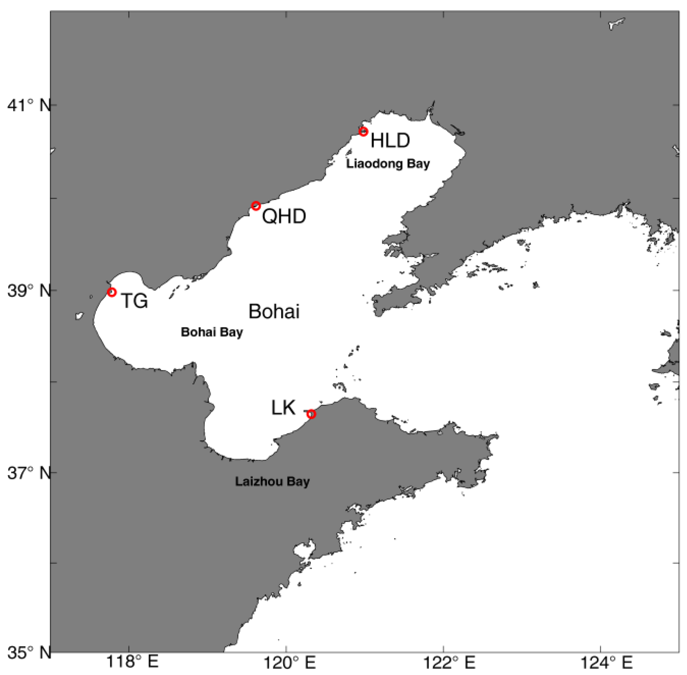
The Bohai Sea, a semienclosed sea that can exchange sea water with the Yellow Sea through the Bohai Strait, has three bays: Laizhou Bay to the south, Liaodong Bay to the north, and Bohai Bay to the west (Figure 1).
Unlike other seas, Bohai Sea is less susceptible to tropical cyclones as few typhoons can move north enough to affect this area. The cold air outbreaks and extratropical cyclones often lead to extreme sea levels in the Bohai Sea [5,6].
In recent years, many studies have been done on the extreme sea level changes both regionally and globally [7,8,9,10,11,12,13,14,15]. Most research indicates that the extreme sea level shows significant increase trend through the 20th century worldwide. However, no uniform conclusions were obtained about the reasons of the changes of extreme sea levels. Many cases show that the extreme sea level changes are caused by the mean sea level changes [7,10,11,12,16,17]. However, other studies indicate that many other factors can affect the extreme sea level changes [15,18,19,20,21,22,23,24], including the change of the astronomical tide, the wind driven components (surge) and the tide–surge interaction.
For the coastal areas in China, only limited studies have been done to analysis the extreme sea level changes [15,25,26], comparing with studies on the mean sea level [27,28,29,30,31] and storm surges [32,33,34,35]. Besides, nearly all these studies concentrated on the Yellow Sea, East China Sea and the South China Sea due to the data limitation. Whether the characteristics of the change of extreme sea level in the Bohai Sea are similar to the other seas around China is not clear. It is essential to promote the understanding of extreme sea levels along the coastline of Bohai Sea for the sake of the coastal protection, future planning and coastal ecosystem conservation.
In this work, hourly sea level data from four tide gauges along the coastline of the Bohai Sea were analyzed to study the changes of the extreme sea level in this area. The harmonic analysis on the tide was conducted for each calendar year [36], and the observed sea level were decomposed into separate components, i.e., the mean sea level (MSL), the astronomical tide and the surges. The inter-decadal variation and long-term changes of each component and the extreme sea levels were studied separately at four tide gauges. The characteristics of the tide–surge interaction were also analyzed. At last, the relationship between the extreme sea level and each component was studied.
2. Data and Methodology
2.1. Data
Since the mid-19th century, tide gauge measurement has been utilized around the world [37,38,39]. Hourly sea level data from four tide gauges (Huludao, Qinhuangdao, Tanggu and Longkou) along the coast of the Bohai Sea were used in this study. These data were obtained from the marine monitoring stations in China (Figure 1), dating from January 1980 to December 2016. All data series are more than 30 years long, which is essential to obtain accurate trends [15]. The data obtained had been quality controlled. In addition, the data were carefully checked for common errors, such as spurious records and data spikes. The missing values, lasting hours, were interpolated [40]. In addition, at Longkou Station, the data in 1990 were not used as data availability was less than 60%.
The Arctic Oscillation (AO) index, a climate index of the state of the atmospheric circulation over the Arctic, was obtained from the National Centers for Environmental Information (NOAA) (https://www.ncdc.noaa.gov/teleconnections/ao/). The Siberian High (SH) index, which represents the intensity of the SH, was calculated using data obtained from the National Center for Atmospheric Research (NCAR) (https://www.esrl.noaa.gov/psd/data/gridded/data.ncep.reanalysis.derived.surface.html). The SH index is defined as follows:
where Pn is the sea level pressure at n point and is the latitude of n. If Pn ≥ 1028 hPa, , else . The selected area is located at 30° N–70° N and 60° E–120° E.
2.2. Characteristics of the Extreme Sea Level and Components
Following Woodworth and Blackman [7], percentile analysis method was used to assess the extreme sea level changes. Three percentile values (99.9%, 99% and 90%) of the observed sea level were calculated. Both the original datasets and ones with the annual median subtracted (50%) were analyzed.
Pugh [36] and Haigh et al. [11] divided the observed sea level into three components: the mean sea level, the astronomical tidal and the nontidal residual. The mean sea level is the mean value of the sea levels during a year. The tidal and surge components were separated using the harmonic analysis method [41].
Three indices, namely annual mean high water (MHW), annual mean low water (MLW) and annual mean tide range (MTW), were used to represent the tidal changes [11]. For the surge (non-tidal residual), the intensity, defined as the total integral of the surge level curve above the threshold, was used as proxy [42]. At all four tide gauges, the 99th percentile of hourly non-tidal sea level variations were used as the threshold and 96 h was used as a time threshold to ensure that the storm surges are independent of one another when count the storm surges.
The tide–surge interaction was also analyzed in this work. Following the work by Haigh et al. [11], the timing of the surge peaks, beyond the threshold, relative to the nearest high tide was calculated. With respect to the timing of high tide, the tide was divided into hour bands. If there were no tide–surge interaction at one tide gauge, the distribution of the surges at each band would be uniform. Otherwise, the number of surges per band would be different. The chi-square test [11,43,44] was calculated to compare the intensity of interaction at each tide gauge. The test statistic equation is computed as
where Ni is the observed number of surges in the i-th tidal band, n = 13 is the number of hour bands (or 25, according to the conditions of the tide), and e is the mean number of surges of total number of phase (n). At the 95% significance level, the test statistic is (critical chi-square value), where the degrees of freedom are thirteen.
The sequential Mann–Kendall test method [45] was used to observe the change of trend of the extreme sea level. This method estimated the series of progressive UF(t) and retrograde UB(t) values which are standardized with mean value of zero and unit standard deviation. The values of xj (j = 1,2,…,n) are compared with xi (i = 2,3,…,n−1). The nj denoted the cases which xj > xi. The test statistic t, the mean E(t), and the variance Var(t) are calculated as follows:
while the progressive UF(t) and the retrograde UB(t) are calculated using the mean and variance as
The equation starts from the first and last data of the time series, respectively. A positive (negative) value of UF(t) or UB(t) indicates an upward (downward) trend in the time series. The intersection point of UF(t) and UB(t) represents the approximate turning point of trend. When UF(t) or UB(t) curve exceed the certain value before or after the intersection point, the trend turning point is considered significant at the corresponding level; for the 5% significant level, the value is 1.96.
2.3. Testing for Significance of Trends and Correlations
The significance of the correlations and trends in this work has been carefully checked using t-test for correlations and Mann–Kendall for trends [45,46,47,48].
The significance of the correlation was test using the t-test in the work. If we want to determine whether the relationship between the X and Y is significant, the null hypothesis can be stated as “X and Y are unrelated”. The p-value (estimated from the t-test) is a number between 0 and 1, which represents the probability that these data would have arisen if the null hypothesis were true. A low p-value (such as 0.05) means that the null hypothesis can be rejected. The correlations can be expressed as the correlation is significant at the 0.05 level.
The Mann–Kendall test is a rank-based nonparametric test for assessing the significance of a trend. The Mann–Kendall test, first introduced by Mann [49], can be defined mostly generally as a test for whether the trend to increase (decrease) with time (monotonic change). The Mann–Kendall test examines whether to reject the null hypothesis (H0: no monotonic trend) and accept the alternative hypothesis (H1: the monotonic trend is present).
The Mann–Kendall trend test has the initial assumption that the H0 is true and the data are convincing beyond a reasonable doubt before H0 is rejected and H1 is accepted. The null hypothesis H0 is that the data {Xi, i = 1,2…,n} are independent and identically distributed. The other hypothesis H1 is that X has a monotonic trend. The statistic S is as follows:
where Xj are the sequential data, n is the dataset length, and if Xj − Xi > 0 the f equals 1, if Xj − Xi = 0 the f equals to 0, else the f equals −1. If n ≥ 8. The statistic S can be regarded as normal distributed with the variance and mean as:
where tm is the number of ties of m. The standardized test statistic Z can be computed as:
M(S) = 0
If S > 0
If S = 0; Z = 0.
If S < 0
The statistic Z has the mean of zero and variance of one. The probability value of p of the Mann–Kendall statistic S can be calculated using the cumulative distribution function as
For the data without trend, p equals 0.5. For the data with a larger positive trend, p value should be closer to 1.0. For the data with a larger negative trend, p value is nearly 0.0.
3. Results and Discussion
We analyzed the characteristics of change of each component (MSL, tide and surge) and the tide–surge interaction. Then, extreme sea levels and the relationship between extreme sea levels and each component were also analyzed.
3.1. Changes of the Mean Sea Level
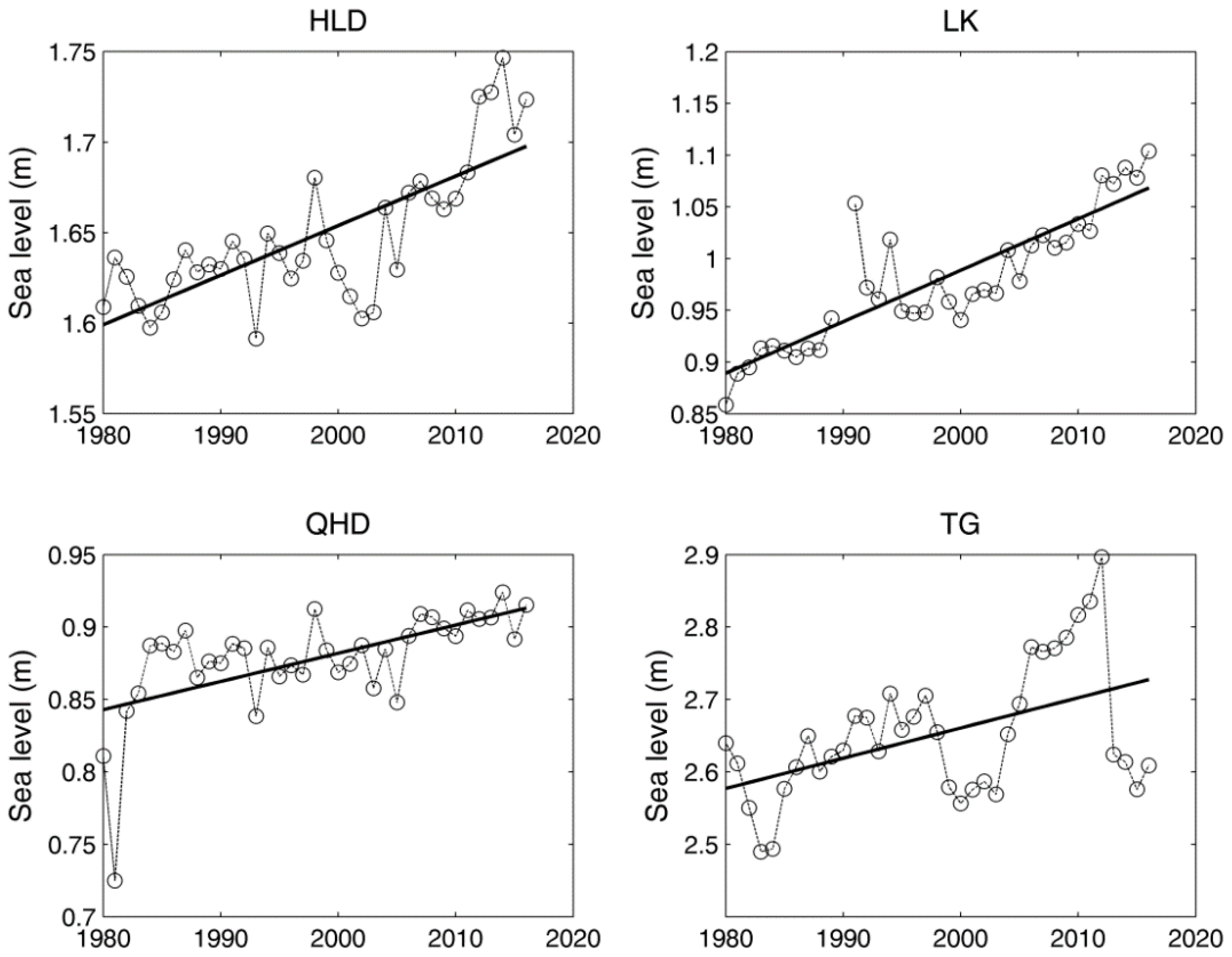
Annual mean sea level of the four tide gauges (Huludao, Longkou, Qinhuangdao and Tanggu) were analyzed. Results (Figure 2) show that clearly decadal variations exist at HLD and TG, with low mean sea levels around 2000, while no clear decadal variability was found at LK and QHD. Mean sea level trends at four tide gauges are listed in Table 1. It shows that linear positive trends are significant at all tide gauges, with rates between 0.2 and 0.5 cm/year. The mean sea level trends we obtained fit well to other results in Bohai area [30,50]. According to the locations of tide gauges (Figure 1), it seems that the sea level rise shows clear spatial characteristics, with positive trend increasing from north to south in the Bohai Sea. It should be noted that uncertainties exist in the trend obtained from the tide gauges, as the rate can be affected by the land movements and data quality. Hu et al. [51,52] found that the land movements vary highly geographically in China.
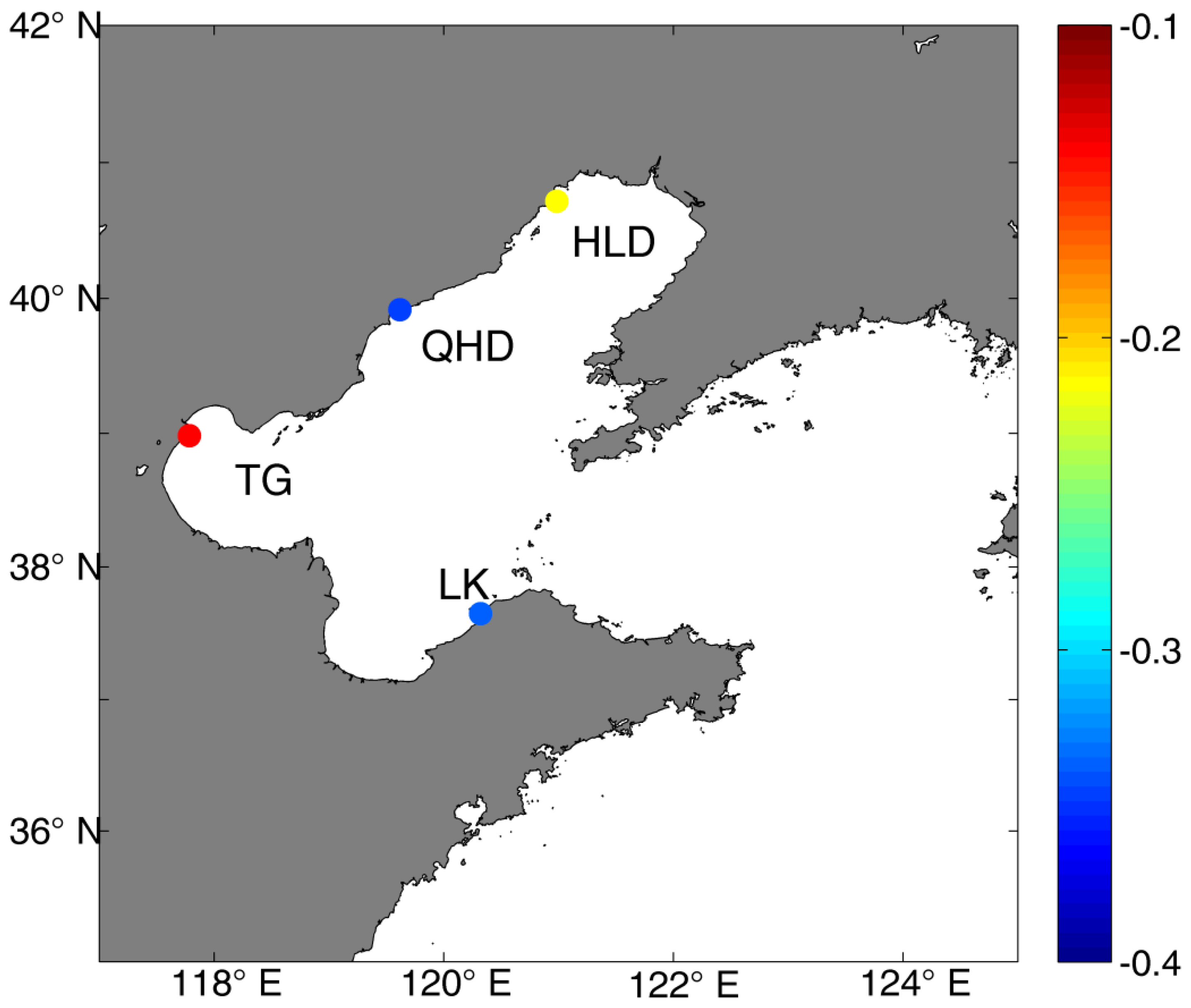
Previous results show that the monsoon in the northwest Pacific Ocean can affect the sea level in the China Sea [53,54,55]. The variations of the East Asian winter monsoon were related to the Pacific decadal oscillation (PDO) [56,57,58]. Studies have found that the sea levels in the northwest Pacific are correlated with the PDO [59,60]. Using the altimetric data, Han and Huang [30] thought that the interannual and long-term sea level variability in the Bohai Sea was negatively correlated with the Pacific decadal oscillation (PDO). The correlations between the sea level at four tide gauges and the PDO were calculated and shown in Figure 3. Results show that the sea level was significant correlated with the PDO at QHD and LK (with p < 0.05). At HLD and TG, the sea level was negatively correlated with the PDO but the correlation was not significant. Han and Huang [30] thought that this correlation represents various regional connections and manifestations, including the ocean temperature and salinity change, and possibly the Kuroshio transport variability.
3.2. Changes of the Tides
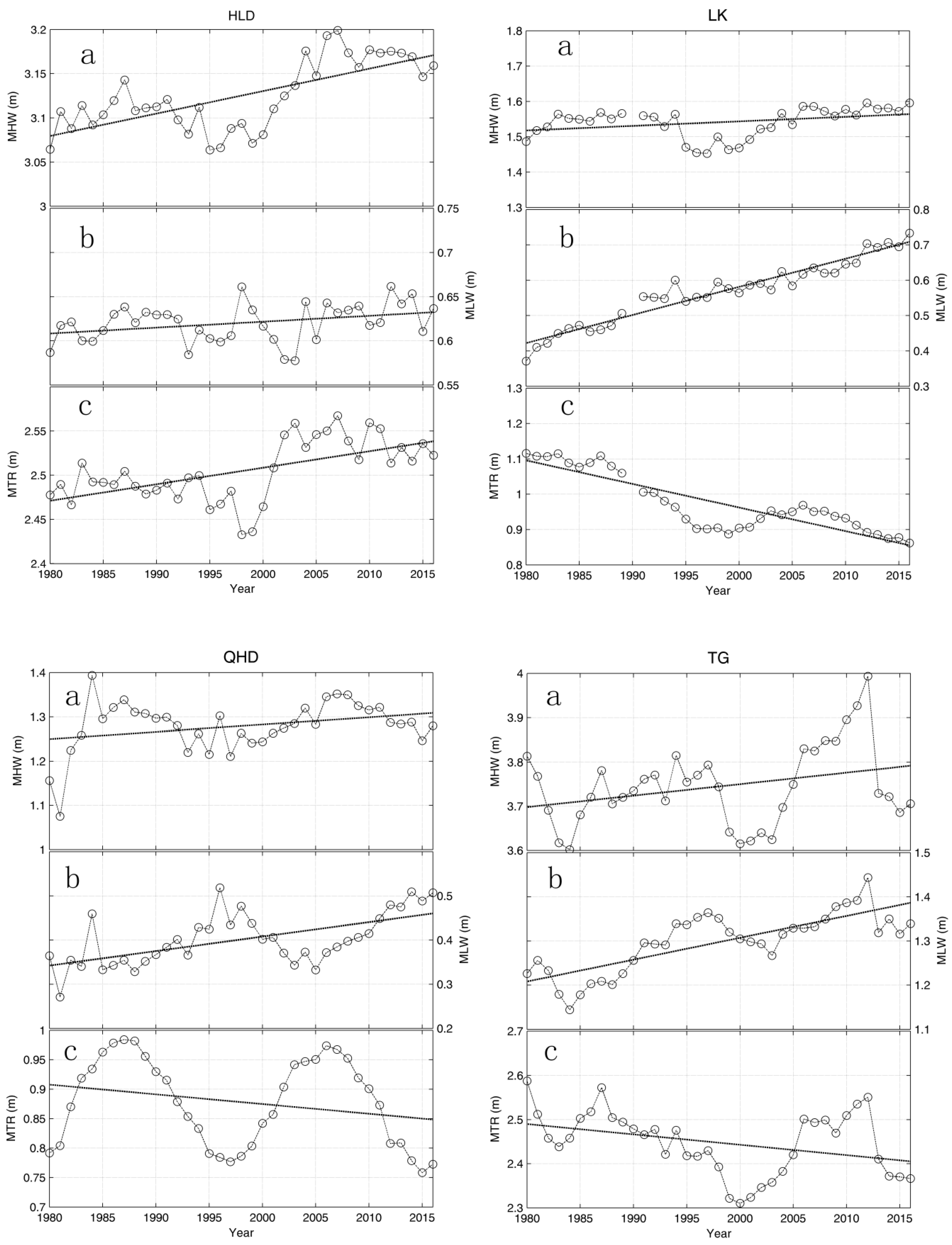
Following Haigh et al. [11], the MHW, MLW and MTR were analyzed to study the characteristics of the tide change at four tide gauges. The results are shown in Figure 4. Annual values show that the tide ranges at HLD and TG are between 2.3 and 2.6 m, which are larger than the other two tide gauges (between 0.7 and 1.1 m).
There is a considerable variability in the MHW and MTR at four tide gauges in the decadal time scales, which may be related to the 18.6-year nodal cycle. The variability of the decadal time scales at MLW was relative weak. The 18.6-year nodal cycle is more significant at the MTR, especially at QHD. The long-term trend rates were calculated (Table 2). The trends show various characteristic at different tide gauges. The trends of the MHW are positive at all four tide gauges, but significant only at HLD. The trends of the MLW are positive at LK, QHD and TG, and are all statistically significant. The increase rate at LK is the largest, about 0.8 cm/year. The MLW does not show clear long-term trend at HLD. The trends of the MTR are negative at LK, QHD and TG, and are statistically significant at LK and TG. However, at HLD, the trend of MTR is significantly positive, about 0.2 cm/year. The increase rate of 0.1–0.3 cm/year in MHW was comparable with the long-term trends in mean sea level (0.2–0.5 cm/year). Thus, relative to extreme sea levels, the increase in MHW also cannot be ignored.
Recent studies found that the regional tidal dynamics may be affected by the sea level changes [61,62]. The correlation between the sea level rise and the tide are listed in Table 2. Results show that the MHW and MLW were significantly correlated with the mean sea level at all four tide gauges. The correlation coefficients range from 0.45 to 0.95. The correlation differs due to the locations, which was caused by the land reclamation along the coast [63,64,65].
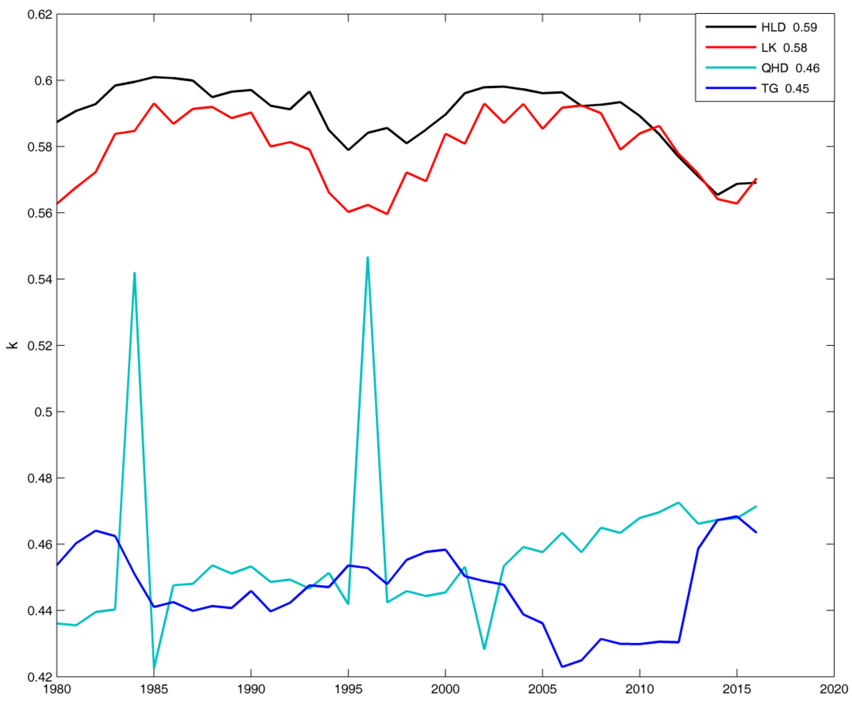
To make the difference between the MSL and the tide clear, k factor method [59] was used. The k factor is a dimensionless reference whose value stands for the difference between MSL and MTR. The value of k can be calculated as below:
A symmetric tide has the k factor of 0.5 [30]. The larger deviation exists between k and 0.5, the larger deviation exists between the changes of tide and mean sea level. Using the tide gauges, the k values at four tide gauges were calculated (Figure 5). Results show that that the tide gauges can be divided into two types according to the values of k: one type includes HLD and LK, and the other includes QHD and TG. The deviation between k and 0.5 was largest at HLD, with mean k value of about 0.59. The deviation was smallest at QHD, with k value of about 0.46. There are two k peaks in QHD, which were caused by the peak values of the MHW. These results were consistent with conclusions obtained by Pelling et al. [65]. They thought that the changes of the tide in the Bohai Sea were both affected by the rapid coastline changes and sea level rise.
3.3. Changes of the Surge
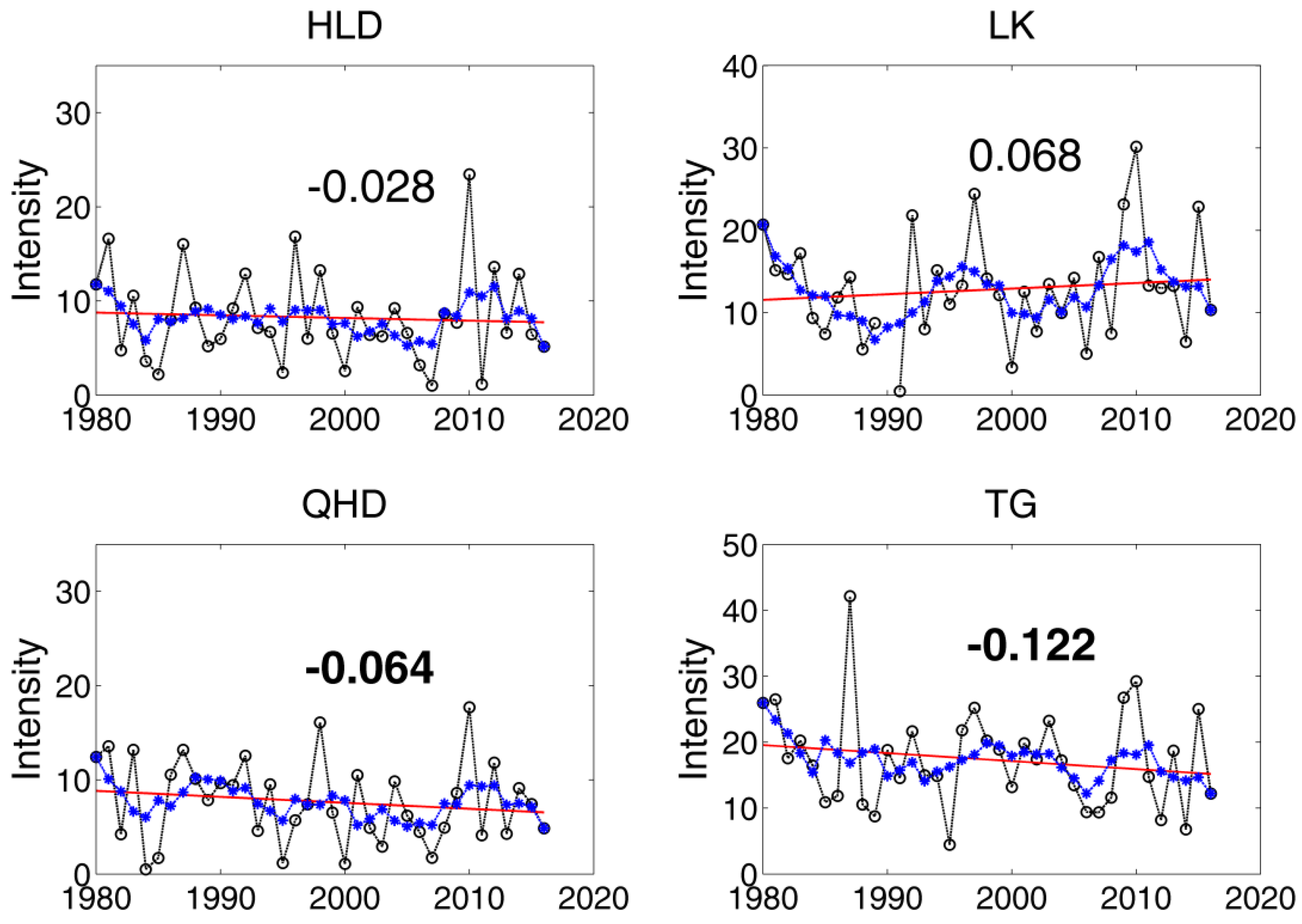
The storm surge intensity described above had been calculated annually at four tide gauges (Figure 6). The 99% surge level was used as the threshold. Results show that the mean value of the surge intensity was largest at TG, about 17.5 h·m. The mean values at HLD and QHD are smallest, about 8.0 h·m. The interannual variations of the storm surge intensities were strong while the decadal variations were relatively weak. The decadal variation at HLD was relatively smaller among the four tide gauges. The intensity tended to be larger around 2010 at HLD. Around 1980, 1995 and 2010, the intensity was relatively high at LK. The decadal variations were similar at QHD and TG, with generally larger values around 1990, 2000 and 2010. The long-term trends at QHD and TG were significantly negative. The long-term trend at HLD was also negative, while a positive trend existed at LK; however, they did not pass the significance test at 95% level.
Researchers found that the surge variability is mostly related to variations of the regional climate [7,10,34]. The storm surges in the Bohai Sea are mostly caused by the cold air outbreaks and extratropical cyclones [5,6,34]. The Arctic Oscillation (AO) and Siberian High (SH) can significant affect the frequency and intensities of cold air outbreaks and extratropical cyclones [66,67,68,69,70,71,72]. When the AO is positive, the surface pressure in the polar region is low, which locks the cold Arctic air in the polar area. In contrast, high pressure in the polar region can help frigid polar air move to middle latitudes. Gong and Ho [73] thought that the warmer winter in almost all of inland extratropical Asia is driven by the weakening of SH.
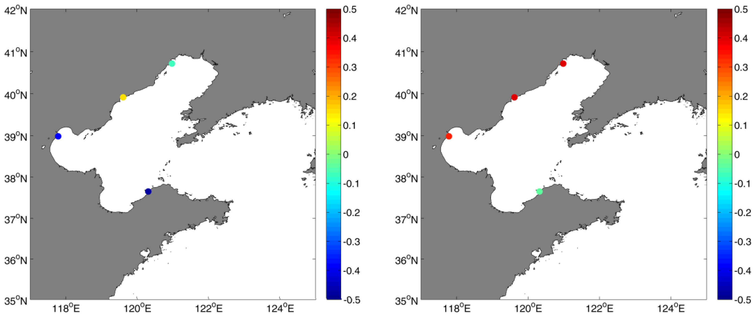
The correlation coefficients between surge intensity and the AO and SH were calculated in this work. Results (Figure 7) show that correlation varies among different tide gauges. The AO and storm surge intensity have significantly negative correlations at LK and TG (with p < 0.05). No significant correlation exists between the AO and storm surge intensity at HLD and QHD. Significant positive correlations between the SH and storm surge intensity can be found at HLD, QHD and TG (with p < 0.05). No significant correlation exists between the SH and storm surge intensity at LK. It seems that the correlations are different due to the location of the tide gauges. The AO index affects the storm surge in the southwest of the Bohai Sea, and the SH affects the storm surge in the northwest of the Bohai Sea.
3.4. The Tide–Surge Interaction
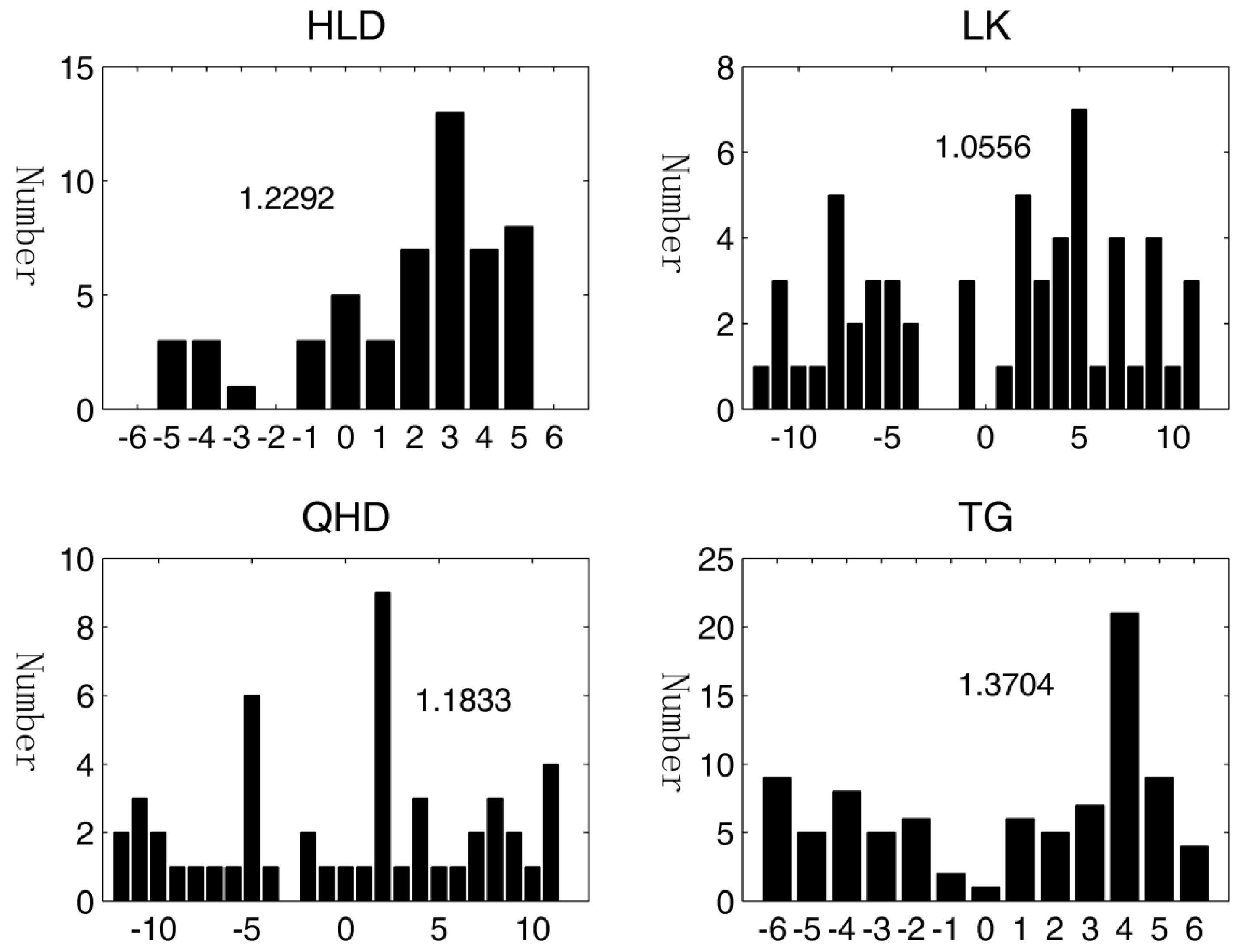
The distribution of peak surges (above 99.9% of sea level) relative to the timing of high tide at four tide gauges were calculated (Section 2.2). The characteristics of the tide–surge interaction are shown in Figure 8. Results show that tide–surge interaction exists at all four tide gauges. The characteristics differ due to their locations. At HLD and TG, the surge often happen at the ebb tide (3–4 h after the high tide). At LK, the distribution has peaks at both rising and falling tide. At QHD, the surges occur mostly at two bands, 5 h before the high tide and 2 h after the high tide. The test statistic was used to quantify the strength of the tide–surge interaction at four tide gauges (values are listed in Figure 7), where T is the length of the data set (year). Results show that the tide–surge interaction is the most significant at TG, and the value of the test statistic is the smallest at LK.
To find whether the tide–surge interaction at four tide gauges have changed or not over the past decades, we plot the phases for all 10-year periods in Figure 9. Results show that the tide–surge interaction at HLD, QHD and TG is quite stable, with only small changes occurring during the past years. At LK, some changes occurred in the tide–surge interaction. We conclude that the tide–surge interaction becomes more stable with the increase of the value of .
3.5. Changes of Extreme Sea Levels
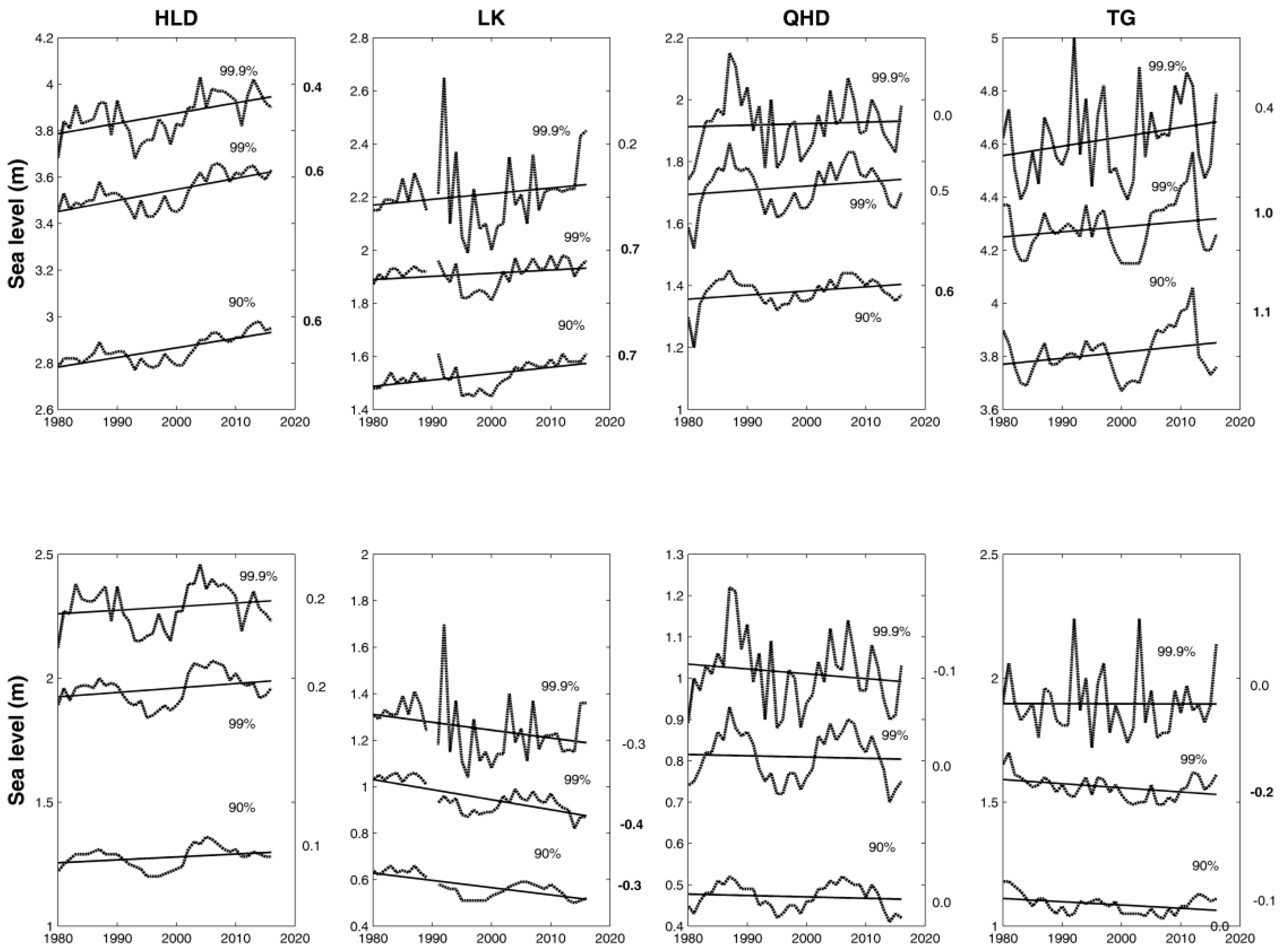
The changes of the extreme sea level at four tide gauges are analyzed in this section. Three percentiles (99.9%, 99% and 90%) of total and reduced (subtracting the annual mean sea level) annual sea level were calculated, as plotted in Figure 10. Clearly, decadal variations exist in the extreme sea levels at all four tide gauges. Results show that the three percentiles all show positive trend at HLD, LK and TG, and most of them are significant. At QHD, these is no obvious trend at the 99.9%, while there are positive trends at 99% and 90% levels. Results also show that the increase rates decrease when the percentile level increase at all four tide gauges. At HLD, the rates of the extreme sea levels are all larger than the rate of the mean sea level (Section 3.1). At LK and QHD, the rates of 99% and 90% are larger than the rates of mean sea level, while the rate of 99.9% is smaller than the rate of the mean sea level. At TG, the rates of 99% and 90% are larger than the rates of mean sea level. Compared with the extreme sea level in other seas in China, the extreme sea level increase rates were smaller [15].
When the percentile time series are subtracted from the annual mean sea level, most of the trends changed to be not significant. Positive trends were still found at HLD. At LK and TG, the trends change to negative. No clear trends exist at QHD. However, marked decadal variability still exist at all four tide gauges.
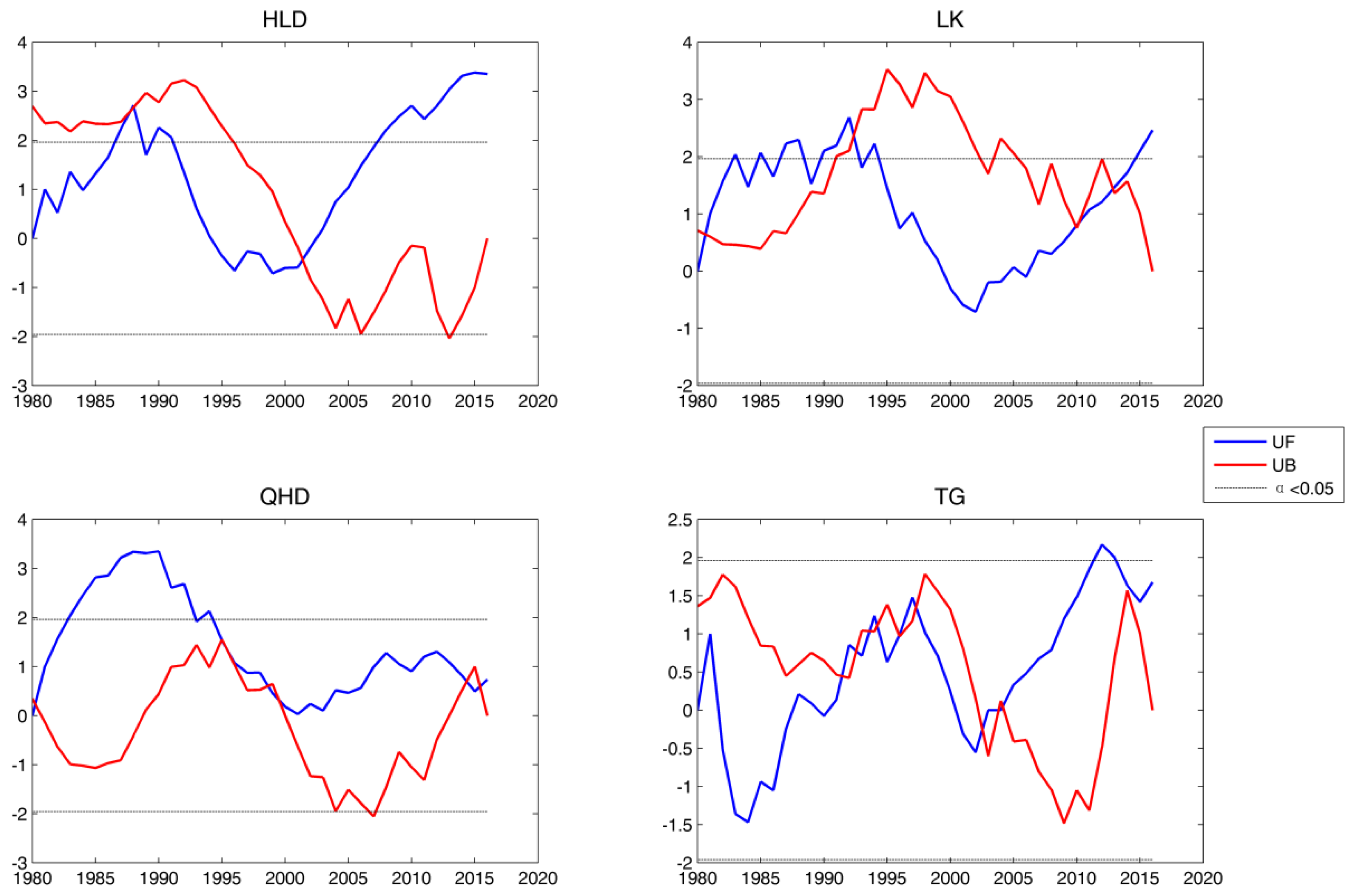
The progressive UF(t) and the retrograde UB(t) series of the sequential Mann–Kendall test against time for 99.9% extreme sea level were calculated (Figure 11). At HLD, significant positive trend in the extreme sea level were observed within the period 1987–1992 and after 2007. Positive trend started from 2003. At LK, significant positive trend in the extreme sea level were observed within the period 1982–1994 and after 2015. At QHD, significant positive trend in the extreme sea level were observed within the period 1982–1994. The positive trend started in 1980 but after 1996 it reduced to approximately a zero trend. At TG, significant positive trend in the extreme sea level were observed within the period 2012–2014. Positive trend started from 2003.
3.6. Relationship between Extreme Sea Level and Components
The relationship between the annual variations of the extreme sea level (the 99.9% level) and the variations of three components (MSL, tide and surge) of sea level were analyzed separately. The surge par is represented by the annual surge intensity. The tide component is represented by the annual mean high level. The correlations were calculated, as listed in Table 3.
Many studies, both at regional [11,15,74,75] and global scales [7], show that the extreme sea level is highly correlated with the mean sea level. In the Bohai area, the results show general consistency. The extreme sea levels were significantly positively correlated to the MSL at HLD, QHD and TG. The correlation is largest at TG, about 0.59. The correlation at LK is also positive but not statistically significant.
The extreme sea levels were significant positive correlated to the tide at all four tide gauges. All correlations are larger than 0.5, especially at HLD (>0.8). It seems that the tide plays more important roles in the changes of extreme sea level in the Bohai area; this conclusion is quite different from other areas along the Chinese coast [15]. As for the surge part, results are different in different locations. The surge shows significant positive correlation to the extreme sea level at LK. However, at the other three tide gauges, no significant correlations exist between the surge and the extreme sea levels. A possible reason is that the distributions of the surge at LK are more uniform than other tide gauges (the tide–surge interaction is smallest at this tide gauge) (Figure 8).
In conclusion, both the mean sea level and tide play important roles in the changes of the extreme sea levels. In the Bohai area, it seems that the changes of the tide play more important roles than the MSLs. At some locations, if the tide–surge interaction is small, the surge may also be important in the changes of extreme sea levels.
4. Conclusions
Using the hourly sea level data from four tide gauges along the coast, the extreme sea levels in the Bohai Sea were analyzed. The variability of the changes of mean sea level, tide and surge were studied separately, and the tide–surge interactions were also analyzed. We then assessed the contributions of the changes of these three components and the tide–surge interaction on the extreme sea level changes.
The mean sea level, tide and surge components were separately analyzed to obtain decadal variability features and long-term trends. Significant increase trends exist at all four tide gauges, with rates ranging from 0.2 to 0.5 cm/year. The rate of sea level rises shows obvious spatial characteristics. The positive trends increase from north to south in the Bohai Sea. Considerable yearly variability of the tide component exists, which is significantly related to the 18.6-year nodal cycle. The MHW increase by 0.1–0.3 cm/year is not small compared to the long-term trends of the mean sea level (0.2–0.5 cm/year). Distinct inter-annual variability and decadal variability exist in the surge component at all four tide gauges. At QHD and TG, the annual surge intensity shows clear long-term decrease trend. The tide–surge interaction was significant but spatially non-uniform at all four tide gauges. No obvious changes were found in the tide–surge interaction at these tide gauges.
The increase of the extreme sea levels during the past decades at all tide gauges is evident, suggesting the clear decadal variability. The extreme sea level and the MSL are significantly positively correlated at HLD, QHD and TG according to the analysis results. Besides, the tide is significantly positively correlated to the extreme sea level at all tide gauges, and all correlation coefficients are larger than 0.5. These indicate that the MSL changes and the tide play important roles in the decadal and long-term changes of the extreme sea level. Moreover, significant positive correlation exists between the surge and extreme sea level at LK, where the tide–surge interaction is smallest among all four tide gauges.
In conclusion, the changes of the mean sea level and tide have significant effects on the changes of the extreme sea levels in the Bohai Sea. Unlike other areas along the Chinese coast, the effects of tide may be more important in this region. At some specific locations where the tide–surge interaction is relatively small, the surge also plays important roles in the changes of extreme sea level.
Author Contributions
Conceptualization, F.J.; Methodology, W.H.; Software, W.H., and L.D.; Validation, L.Q., Z.J., L.Y., and L.K.; Writing—Original Draft Preparation, F.J.; Writing—Review & Editing, L.Q.; Visualization, L.D.; Supervision, F.J.; Project Administration, F.J.; Funding Acquisition, F.J. and L.D.
Funding
This work was funded by the National Key Research Projects (2017YFC1404200 and 2016YFC1401900), and the National Natural Science Foundation of China (Grant No. 41706020 and No. 41406032) and Open Fund if the Key Laboratory of Research on Marine Hazards Forecasting.
Acknowledgments
We thanks for the data supplied from the marine monitoring stations in China.
Conflicts of Interest
The authors declare no conflict of interest.
References
- United Nations Framework Convention on Climate Change. COP21 Paris Agreement. Available online: http://unfccc.int/2860.php (accessed on 12 December 2015).
- Mechler, R.; Bouwer, L.M.; Linnerooth-Bayer, L.; Hochraniner-Stigler, S.; Aerts, J.C.H.; Surminski, S.; Williges, K. Managing unnatural disaster risk from climate extremes. Nat. Clim. Chang. 2014, 4, 235–237. [Google Scholar] [CrossRef]
- Cutter, S.L.; Gall, M. Sendai targets at risk. Nat. Clim. Chang. 2015, 5, 707–709. [Google Scholar] [CrossRef]
- Vousdoukas, M.I.; Mentaschi, L.; Voukouvalas, E.; Verlaan, M.; Feyen, L. Extreme sea levels on the rise along Europe’s coasts. Earth’s Future 2007, 5, 304–323. [Google Scholar] [CrossRef]
- Feng, S. Introduction to Storm Surge; Science Press: Beijing, China, 1982; p. 241. (In Chinese) [Google Scholar]
- Zhao, P.; Jiang, W. A numerical study of storm surges caused by cold-air outbreaks in the Bohai Sea. Nat. Hazards 2011, 59, 1–15. [Google Scholar] [CrossRef]
- Woodworth, P.L.; Blackman, D.L. Evidence for systematic changes in extreme high water since the mid-1970s. J. Clim. 2004, 17, 1190–1197. [Google Scholar] [CrossRef]
- Méndez, F.J.; Menéndez, M.; Luceño, A.; Losada, I.J. Analyzing monthly extreme sea levels with a time-dependent GEV model. J. Atmos. Ocean. Technol. 2007, 24, 894–911. [Google Scholar] [CrossRef]
- Woodworth, P.L.; Flather, R.A.; Williams, J.A.; Wakelin, S.L.; Jevrejeva, S. The dependence of UK extreme sea levels and storm surges on the North Atlantic Oscillation. Cont. Shelf Res. 2007, 27, 935–946. [Google Scholar] [CrossRef]
- Marcos, M.; Tsimplis, M.N.; Shaw, A.G.P. Sea level extremes in southern Europe. J. Geophys. Res. Oceans 2009, 114, C1. [Google Scholar] [CrossRef]
- Haigh, I.; Rober, N.; Neil, W. Assessing changes in extreme sea levels: Application to the English Channel, 1900–2006. Cont. Shelf Res. 2010, 30, 1042–1055. [Google Scholar] [CrossRef]
- Menéndez, M.; Woodworth, P.L. Changes in extreme high water levels based on a quasi-global tide-gauge data set. J. Geophys. Res. Oceans 2010, 115, C10. [Google Scholar] [CrossRef]
- Mudersbach, C.; Wahl, T.; Haigh, I.D.; Jensen, J. Trends in high sea levels of German North Sea gauges compared to regional mean sea level changes. Cont. Shelf Res. 2013, 65, 111–120. [Google Scholar] [CrossRef]
- Weisse, R.; Bellafiore, D.; Menéndez, M.; Méndez, F.; Nicholls, R.J.; Umgiesser, G.; Willems, P. Changing extreme sea levels along European coasts. Coast. Eng. 2014, 87, 4–14. [Google Scholar] [CrossRef] [Green Version]
- Feng, J.; von Storch, H.; Jiang, W.; Weisse, R. Assessing changes in extreme sea levels along the coast of China. J. Geophys. Res. Ocean 2015, 120, 8039–8051. [Google Scholar] [CrossRef] [Green Version]
- D’Onofrio, E.E.; Fiore, M.M.E.; Pousa, J.L. Changes in the regime of storm surges in Buenos Aires, Argentinal. J. Coast. Res. 2008, 24, 260–265. [Google Scholar] [CrossRef]
- Tsimplis, M.N.; Shaw, A.G.P. Seasonal sea level extremes in the Mediterranean Sea and at the Atlantic European coasts. Nat. Hazards Earth Syst. Sci. 2010, 10, 1457–1475. [Google Scholar] [CrossRef] [Green Version]
- Johansson, M.; Bomann, H.; Kahma, K.K.; Launiainen, J. Trends in sea level variability in the Baltic Sea. Boreal Environ. Res. 2001, 6, 159–179. [Google Scholar]
- Church, J.A.; White, N.J.; Coleman, R.; Lambeck, K.; Mitrovica, J.X. Estimates of the regional distribution of sea level rise over the 1950–2000 period. J. Clim. 2004, 17, 2609–2625. [Google Scholar] [CrossRef]
- Ullmann, A.; Pirazzoli, P.A.; Tomasin, A. Sea surges in Camargue: trends over the 20th century. Cont. Shelf Res. 2007, 27, 922–934. [Google Scholar] [CrossRef]
- Ullmann, A.; Moron, V. Weather regimes and sea surge variations over the Gulf of Lions (French Mediterranean coast) during the 20th century. Int. J. Climatol. 2008, 28, 159–171. [Google Scholar] [CrossRef] [Green Version]
- Letetrel, C.; Marcos, M.; Matín Míguez, B.; Woppelmann, G. Sea level extremes in Marseille during 1885–2008. Cont. Shelf Res. 2010, 30, 1267–1274. [Google Scholar] [CrossRef]
- Ullmann, A.; Monbaliu, J. Changes in atmospheric over the North Atlantic and sea-surge variations along the Belgian coast during the twentieth century. Int. J. Climatol. 2010, 30, 558–568. [Google Scholar] [CrossRef]
- Wahl, T.; Chambers, D.P. Evidence for multidecadal variability in US extreme sea level records. J. Geophys. Res. Oceans 2015, 120, 1527–1544. [Google Scholar] [CrossRef] [Green Version]
- Feng, X.; Tsimplis, M.N. Sea level extremes at the coasts of China. J. Geophys. Res. Oceans 2014, 119, 1593–1608. [Google Scholar] [CrossRef] [Green Version]
- Feng, J.; Jiang, W. Extreme water level analysis at three stations on the coast of the Northwestern Pacific Ocean. Ocean Dyn. 2015, 65, 1383–1397. [Google Scholar] [CrossRef]
- Ding, X.; Zheng, D.; Chen, Y.; Chao, J.; Li, Z. Sea level change in Hong Kong from tide gauge measurements of 1954–1999. J. Geodesy 2001, 74, 683–689. [Google Scholar] [CrossRef]
- Yu, Y.; Yu, Y.; Zuo, J. Effect of sea level variation on tidal characteristic values for the East China Sea. China Ocean Eng. 2003, 17, 369–382. [Google Scholar]
- Zuo, J.; Du, L.; Alvaro, P. The characteristic of near-surface velocity during upwelling season on the northern Portugal shelf. J. Ocean Univ. China 2007, 6, 213–225. [Google Scholar] [CrossRef]
- Han, G.Q.; Huang, W.G. Pacific decadal oscillation and sea level variability in the Bohai, Yellow and East China Seas. J. Phys. Oceanogr. 2008, 38, 2772–2783. [Google Scholar] [CrossRef]
- Zuo, J.; He, Q.Q.; Chen, C.L.; Chen, M.X.; Xu, Q. Sea level variability in East China Sea and its response to ENSO. Water Sci. Eng. 2012, 5, 164–174. [Google Scholar] [CrossRef]
- Feng, J.; Jiang, W.; Bian, C. Numerical prediction of storm surge in the Qingdao area under the impact of climate change. J. Ocean Univ. China 2014, 13, 539–551. [Google Scholar] [CrossRef]
- Zhao, C.; Ge, J.; Ding, P. Impact of Sea Level Rise on Storm Surges around the Changjiang Estuary. J. Coast. Res. 2014, 68, 27–34. [Google Scholar] [CrossRef]
- Feng, J.; von Storch, H.; Weisse, R.; Jiang, W. Changes of storm surges in the Bohai Sea derived from a numerical model simulation, 1961–2006. Ocean Dyn. 2016, 66, 1301–1315. [Google Scholar] [CrossRef]
- Mo, D.; Hou, Y.; Li, J.; Liu, Y. Study on the storm surges induced by cold waves in the Northern East China Sea. J. Mar. Syst. 2016, 160, 26–39. [Google Scholar] [CrossRef]
- Pugh, D.J. Tide, Surge and Mean Sea Level: A Handbook for Engineers and Scientists; John Wiley: Chichester, UK, 1987; p. 472. [Google Scholar]
- Douglas, B.C. Global sea level rise. J. Geophys. Res. 1991, 96, 6981–6992. [Google Scholar] [CrossRef]
- Jevrejeva, S.; Grinsted, A.; Moore, J.; Holgate, S. Nonlinear trends and multiyear cycles in sea level records. J. Geophys. Res. 2006, 111, C09. [Google Scholar] [CrossRef]
- Church, J.A.; White, N.J.; Konikow, L.; Domingues, C.; Goley, J.; Rignot, E. Revisiting the Earth’s sea level and energy budget from 1961 to 2008. Geophys. Res. Lett. 2011, 38, L18601. [Google Scholar] [CrossRef]
- Wang, H.; Liu, K.; Fan, W.; Fan, Z. Data uniformity revision and variations of the sea level of the western Bohai Sea. Mar. Sci. Bull. 2013, 32, 256–264, (Chinese with English abstract). [Google Scholar]
- Pawlowicz, R.; Beardsley, B.; Lentz, S. Classical tidal harmonic analysis including error estimates in MATLAB using T-TIDE. Comput. Geosci. 2002, 28, 929–937. [Google Scholar] [CrossRef]
- Zhang, K.; Douglas, B.C.; Leatherman, S.P. Twentieth-century storm activity along the US east coast. J. Clim. 2000, 13, 1748–1761. [Google Scholar] [CrossRef]
- Horsburgh, K.J.; Wilson, C. Tide-surge interaction and its role in the distribution of surge residuals in the North Sea. J. Geophys. Res. 2007, 112, C08003. [Google Scholar] [CrossRef]
- Antony, C.; Unnikrishnan, A.S. Observed characteristics of tide-surge interaction along the east coast of India and the head of Bay of Bengal. Estuar. Coast. Shelf Sci. 2013, 131, 6–11. [Google Scholar] [CrossRef]
- Rashid, M.M.; Beecham, S.; Chowdhury, R.K. Assessment of trends in point rainfall using continuous Wavelet Transforms. Adv. Water Resour. 2015, 82, 1–15. [Google Scholar] [CrossRef]
- Kulkarni, A.; von Storch, H. Monte Carlo experiments on the effect of serial correlation on the Mann-Kendall-test of trends. Meteor Z. 1995, 4, 82–85. [Google Scholar] [CrossRef]
- Von Storch, H.; Zwiers, F.W. Statistical Analysis in Climate Research; Cambridge University Press: Cambridge, UK, 1999; p. 495. [Google Scholar]
- Gharineiat, Z.; Deng, X. Description and assessment of regional sea-level trends and variability from altimetry and tide gauges at the northern Australian coast. Adv. Space Res. 2018, 61, 2540–2554. [Google Scholar] [CrossRef]
- Mann, H.B. Nonparametric tests against trend. Econometrica 1945, 13, 245–259. [Google Scholar] [CrossRef]
- China Sea Level Bulletin. Available online: http://www.soa.gov.cn/zwgk/hygb/zghpmgb/201804/t20180423_61104.html (accessed on 23 April 2017).
- Hu, H.M.; Huang, L.; Yang, G.H. Recent crustal vertical movement in the Changjiang River delta and its adjacent area (in Chinese with English abstract). Acta Geogr. Sin. 1992, 47, 22–30. [Google Scholar]
- Hu, H.M.; Huang, L.; Yang, G.H. Recent vertical crustal deformation in the coastal area of eastern China (in Chinese with English abstract). Sci. Geol. Sin. 1993, 28, 270–278. [Google Scholar]
- Liu, Q.; Jia, Y.; Wang, X.; Yang, H. On the annual cycle characteristics of the sea surface height in South China Sea. Adv. Atmos. Sci. 2001, 18, 613–622. [Google Scholar]
- Jia, Y.; Liu, Q. Variation of Sea Surface Height in the South China Sea. In Proceedings of the Symposium on 15 Years of Progress in Radar Altimetry; Danesy, D., Ed.; ESA Publications Division: Noordwijk, The Netherlands, 2006. [Google Scholar]
- Huang, L.; Sun, J.; Yang, Y.Q.; Yuan, Y.F. Sea surface Height (SSH) change and its relationship with wind stress in the north Pacific ocean. Oceanol. Limnol. Sin. 2013, 44, 111–119, (In Chinese with English Abstract). [Google Scholar]
- Overland, J.E.; Adams, J.M.; Bond, N.A. Decadal variability of the Aleutian Low and its relation to high-latitude circulation. J. Clim. 1999, 12, 1542–1548. [Google Scholar] [CrossRef]
- Nakamura, H.; Izumi, T.; Sampe, T. Interannual and decadal modulations recently observed in the Pacific storm track activity and East Asian winter monsoon. J. Clim. 2002, 15, 1855–1874. [Google Scholar] [CrossRef]
- Kao, P.; Hung, C.; Hsu, H.H. Decadal variation of the east Asian Winter Monsoon and Pacific Decadal Oscillation. Terr. Atmos. Ocean. Sci. 2016, 27, 617–624. [Google Scholar] [CrossRef]
- Casey, K.S.; Adamec, D. Sea surface temperature and sea surface height variability in the North Pacific Ocean from 1993 to 1999. J. Geophys. Res. 2002, 107, C8. [Google Scholar] [CrossRef]
- Gordon, A.L.; Giulivi, C.F. Pacific decadal oscillation and sea level in the Japan/East Sea. Deep-Sea Res. 2004, 51, 653–663. [Google Scholar] [CrossRef]
- Pickering, M.D.; Wells, N.C.; Horsburgh, K.J.; Green, J.A.M. The impact of future sea-level rise on the European Shelf tides. Cont. Shelf Res. 2012, 35, 1–15. [Google Scholar] [CrossRef]
- Ward, S.L.; Green, J.A.M.; Pelling, H.E. Tides, sea-level rise and tidal power extraction on the European Shelf. Ocean Dyn. 2012, 62, 1153–1167. [Google Scholar] [CrossRef]
- Zhang, J.; Wang, J. Combined impacts of MSL rise and the enlarged tidal range on the engineering design standard in the areas around the Huanghe River mouth. Mar. Sci. Bull. 1999, 18, 1–9. [Google Scholar]
- Li, X.; Sun, X.; Wang, S.; Ye, F.; Li, Y.; Li, X. Characteristic analysis of Tianjin offshore tide. Mar. Sci. Bull. 2011, 13, 40–49. [Google Scholar]
- Pelling, H.E.; Uehara, K.; Green, J.A.M. The impact of coastline changes and sea level rise on the tides in the Bohai Sea, China. J. Geophys. Res. Ocean 2013, 118, 3462–3472. [Google Scholar] [CrossRef]
- Ding, Y. Build-up, air mass transformation and propagation of Siberian high and its relations to cold surge in East Asia. Meteorog. Atmos. Phys. 1990, 44, 281–292. [Google Scholar] [CrossRef]
- Li, X. A Study of Cold Waves in East Asia. In Meteorology (1919–1949): Offprint of Scientific Works (in Chinese); Academia Sinica; Science Press: Beijing, China, 1955; pp. 35–117. [Google Scholar]
- Gregory, J.M.; Martyn, P.C.; Mark, C.S. Trends in Northern Hemisphere surface cyclone frequency and intensity. J. Clim. 2001, 14, 2763–2768. [Google Scholar] [CrossRef]
- Wang, Z.; Ding, Y. Climate change of the cold wave frequency of China in the last 53 years and the possible reasons. Chin. J. Atmos. Sci. 2006, 30, 1068–1076, (In Chinese with English Abstract). [Google Scholar]
- Zuo, X.; Alexander, L.V.; Paker, D.; Casear, J. Variations in severe storms over China. Geophys. Res. Lett. 2006, 33, L17701. [Google Scholar] [CrossRef]
- Jeong, J.; Ou, T.; Linderholm, H.W.; Kim, B.; Kug, J.; Chen, D. Recent recovery of the Siberian High intensity. J. Geol. Phys. Res. Atmos. 2011, 116, D23012. [Google Scholar] [CrossRef]
- Francis, J.A.; Vavrus, S.J. Evidence linking Arctic amplification to extreme weather in mid-latitude. Geophys. Res. Lett. 2012, 39, L6801. [Google Scholar] [CrossRef]
- Gong, D.Y.; Ho, C.H. The Siberian High and climate change over middle to high-latitude Asia. Theor. Appl. Climatol. 2002, 72, 1–9. [Google Scholar] [CrossRef]
- Bromirski, P.D.; Flick, R.E.; Canyan, D.R. Storminess variability along the California Coast: 1858–2000. J. Clim. 2003, 16, 982–993. [Google Scholar] [CrossRef]
- Pirazzoli, P.; Costa, S.; Dornbusch, U.; Tomain, A. Recent evolution of surge-related events and assessment of coastal flooding risk on the eastern coasts of the English Channel. Ocean Dyn. 2006, 56, 1–15. [Google Scholar] [CrossRef]
Figure 1.
Four tide gauges, Huludao (HLD), Qinhuangdao (QHD), Tanggu (TG) and Longkou (LK), along the coast of the Bohai Sea; and three bays in the Bohai Sea, Liaodong Bay, Bohai Bay and Laizhoy Bay.
Figure 1.
Four tide gauges, Huludao (HLD), Qinhuangdao (QHD), Tanggu (TG) and Longkou (LK), along the coast of the Bohai Sea; and three bays in the Bohai Sea, Liaodong Bay, Bohai Bay and Laizhoy Bay.

Figure 2.
Mean sea level (curve line) and fitted linear trends (straight line) at four tide gauges: HLD (Huludao), LK (Longkou), QHD (Qinhuangdao) and TG (Tanggu).
Figure 2.
Mean sea level (curve line) and fitted linear trends (straight line) at four tide gauges: HLD (Huludao), LK (Longkou), QHD (Qinhuangdao) and TG (Tanggu).

Figure 3.
Correlation between the sea level and the PDO at four tide gauges.

Figure 4.
Three indices at four tide gauges: annual mean high water (MHW) (a); annual mean low water (MLW) (b); and annual mean tide range (MTR) (c). The dotted lines show the linear trends.
Figure 4.
Three indices at four tide gauges: annual mean high water (MHW) (a); annual mean low water (MLW) (b); and annual mean tide range (MTR) (c). The dotted lines show the linear trends.

Figure 5.
The annual k factor values (y-axis) and the mean value (in the legend) at all four tide gauges.
Figure 5.
The annual k factor values (y-axis) and the mean value (in the legend) at all four tide gauges.

Figure 6.
Storm surge intensity (m·h) at HLD, LK, QHD and TG: linear trend (blue line) and five-year running mean (red line). The numbers in the figure are the long-term change rate (m·h/year).
Figure 6.
Storm surge intensity (m·h) at HLD, LK, QHD and TG: linear trend (blue line) and five-year running mean (red line). The numbers in the figure are the long-term change rate (m·h/year).

Figure 7.
Correlations between storm surge intensity and the AO (left); and correlations between storm surge intensity and SH (right).
Figure 7.
Correlations between storm surge intensity and the AO (left); and correlations between storm surge intensity and SH (right).

Figure 8.
The tide–surge interaction at all four tide gauges, numbers listed in the figure is the value of ; y axes are the numbers, and x axes are the hours before and after the high tide.
Figure 8.
The tide–surge interaction at all four tide gauges, numbers listed in the figure is the value of ; y axes are the numbers, and x axes are the hours before and after the high tide.

Figure 9.
Distributions of surge peaks for all 10-year periods at four tide gauges; y axes are the percentage, and x axes are the hours before and after the high tide.
Figure 9.
Distributions of surge peaks for all 10-year periods at four tide gauges; y axes are the percentage, and x axes are the hours before and after the high tide.

Figure 10.
Time series of percentiles of total (top) and reduced (bottom) sea level for HLD, LK, QHD and TG; the straight lines are the linear trends, and their change rates (cm/year) are listed at right of the figure (in bold if significant at 95%).
Figure 10.
Time series of percentiles of total (top) and reduced (bottom) sea level for HLD, LK, QHD and TG; the straight lines are the linear trends, and their change rates (cm/year) are listed at right of the figure (in bold if significant at 95%).

Figure 11.
The MK-values (y axes) for sequential Mann–Kendall test against time (year, x axes) for 99.9% extreme sea level at four tide gauges; the blue line represents the progressive series UF(t), the red line represent retrograde series UB(t), and the dotted lines are the confidence limits ().
Figure 11.
The MK-values (y axes) for sequential Mann–Kendall test against time (year, x axes) for 99.9% extreme sea level at four tide gauges; the blue line represents the progressive series UF(t), the red line represent retrograde series UB(t), and the dotted lines are the confidence limits ().


Table 1.
Mean sea level trends at four tide gauges a.
| Tide Gauge | Period | Trend (cm/year) |
|---|---|---|
| Huludao | 1980–2016 | 0.27 |
| Longkou | 1980–2016 | 0.5 |
| Qinhuangdao | 1980–2016 | 0.2 |
| Tanggu | 1980–2016 | 0.4 |
a Trends with significance at the 95% confidence level are italicized.
Table 2.
The linear trends of the MHW, MLW and MTR (cm/year), and correlations between the tide and mean sea level (C).
Table 2.
The linear trends of the MHW, MLW and MTR (cm/year), and correlations between the tide and mean sea level (C).
| HLD | LK | QHD | TG | |||||
|---|---|---|---|---|---|---|---|---|
| Trend | C | Trend | C | Trend | C | Trend | C | |
| MHW | 0.2 | 0.47 | 0.1 | 0.45 | 0.2 | 0.77 | 0.3 | 0.92 |
| MLW | 0 | 0.64 | 0.8 | 0.95 | 0.4 | 0.61 | 0.5 | 0.64 |
| MTR | 0.2 | 0.13 | −0.7 | −0.81 | −0.3 | 0.11 | −0.2 | 0.55 |
Table 3.
Correlations between the extreme sea level and components.
| Tide Gauge | MSL | Tide | Surge |
|---|---|---|---|
| HLD | 0.34 | 0.82 | 0.05 |
| LK | 0.28 | 0.53 | 0.38 |
| QHD | 0.46 | 0.66 | 0.10 |
| TG | 0.59 | 0.60 | 0.27 |
© 2018 by the authors. Licensee MDPI, Basel, Switzerland. This article is an open access article distributed under the terms and conditions of the Creative Commons Attribution (CC BY) license (http://creativecommons.org/licenses/by/4.0/).
Share and Cite
MDPI and ACS Style
Feng, J.; Li, D.; Wang, H.; Liu, Q.; Zhang, J.; Li, Y.; Liu, K. Analysis on the Extreme Sea Levels Changes along the Coastline of Bohai Sea, China. Atmosphere 2018, 9, 324. https://doi.org/10.3390/atmos9080324
AMA Style
Feng J, Li D, Wang H, Liu Q, Zhang J, Li Y, Liu K. Analysis on the Extreme Sea Levels Changes along the Coastline of Bohai Sea, China. Atmosphere. 2018; 9(8):324. https://doi.org/10.3390/atmos9080324
Chicago/Turabian StyleFeng, Jianlong, Delei Li, Hui Wang, Qiulin Liu, Jianli Zhang, Yan Li, and Kexiu Liu. 2018. "Analysis on the Extreme Sea Levels Changes along the Coastline of Bohai Sea, China" Atmosphere 9, no. 8: 324. https://doi.org/10.3390/atmos9080324
Note that from the first issue of 2016, this journal uses article numbers instead of page numbers. See further details here.