Application of Python Scripting Techniques for Control and Automation of HEC-RAS Simulations

Abstract

The purpose of the paper was to present selected techniques for the control of river flow and sediment transport computations with the programming language Python. The base software for modeling of river processes was the well-known and widely used HEC-RAS. The concepts were tested on two models created for a single reach of the Warta river located in the central part of Poland. The ideas described were illustrated with three examples. The first was a basic simulation of a steady flow run from the Python script. The second example presented automatic calibration of model roughness coefficients with Nelder-Mead simplex from the SciPy module. In the third example, the sediment transport was controlled by Python script. Sediment samples were accessed and changed in the sediment data file stored in XML format. The results of the sediment simulation were read from HDF5 files. The presented techniques showed good effectiveness of this approach. The paper compared the developed techniques with other, earlier approaches to control of HEC-RAS computations. Possible further developments were also discussed.

1. Introduction

River flow modeling is a very popular approach in science and education, as well as in small, medium-size, and large technical projects in the areas of water management [1,2], river regulation [3,4], sediment transport [5], flood protection [6], and many others [7,8]. There are several professionally prepared and widely used commercial and non-commercial models for river flow, e.g., HEC-RAS [9], MIKE 11 [10], Delft Sobek [11], BASEMENT by ETH [12], and SRH1D [13]. The first of the mentioned models, HEC-RAS, is very specific. The acronym HEC means Hydrologic Engineering Center, and it is the name of the software developer. The second element, RAS, means River Analysis System. It defines the software application area which is focused on modeling of flow and transport processes in rivers, floodplains, and reservoirs. All of the modeled elements are solved with highly accurate numerical methods [9]. Additionally, HEC-RAS is freeware with a professionally developed graphical user interface. It makes application of the software easier, and it is considered to be the reason that HEC-RAS is so popular. Today a strong focus on modeling of uncertainty related to river processes is observed. It is a particularly crucial problem in the areas of model calibration [14,15], sediment transport [16,17], and flood hazard mapping [18,19]. The effective management of such computational tasks is not possible without automation of simulation and integration with other tools, e.g., GIS software. The examples analyzed in the paper present crucial automation techniques for the mentioned applications.

The main purpose of this paper is to present selected techniques for controlling HEC-RAS computations with the programming language Python. Control of river flow simulations with external scripts opens several new opportunities in the fields of flood hazard assessment, water management, and river hydraulics. It also enables application of more sophisticated methods in these fields, such as sensitivity analysis, automatic model calibration, and probabilistic flood mapping. The control of the HEC-RAS computations is possible due to the fact that this package is installed with the Component Object Module (COM). This COM library of methods is called HECRASController. The COM library enables outer access to the computational elements of HEC-RAS. The discussion presented here is focused on three specific examples. The ideas presented are not limited to the basic running of flow model simulation. Some concepts are aimed at integration of HEC-RAS with specific tools available in Python modules, e.g., SciPy, while others extend the capabilities of HECRASController and open access to more sophisticated data formats, e.g., XML (eXtensible Markup Language) and HDF5 (Hierarchical Data Format 5).

The HECRASController is a collection of Visual Basic subroutines and functions within the HEC-RAS package. It may be effectively used with VBA (Visual Basic for Applications) in Excel [20,21]. The main capabilities of this collection include running HEC-RAS and particular HEC-RAS editors, running computations plans, reading results of flow simulation, etc. One very interesting feature is the possibility of manipulation of roughness coefficients. It is a very important problem studied by many researchers, e.g., Yang et al. [22] and Lacasta et al. [23]. This capability is implemented in AHYDRA software [24]. The AHYDRA supports calibration of roughness coefficients and boundary conditions for steady flow conditions. The software cooperates with the initially configured HEC-RAS model, enabling automatic change of settings.

The capabilities of HECRASController are still limited. Even the main author promoting the use of this programming tool, Goodell [20,21], advises manipulation of the HEC-RAS data files in ASCII format. Another problem is the use of Visual Basic/VBA. Although it is a very handy programming language, its use is rather limited and still narrowing, e.g., VBA was replaced in ArcGIS by Python and its extension ArcPy. Hence, other languages are also implemented to handle HECRASController, e.g., MATLAB [25].

Python [26] is one of the most popular programming languages used today worldwide. It is easily applied in practical cases, as well as in highly scientific problems [27,28]. Its popularity follows from two factors: (1) relative simplicity and (2) a broad range of application areas. Considering the specific problem considered here, Python has several advantages and unique features. They include very easy access to text files in standard form, e.g., [26]; several specific libraries included, e.g., [29,30,31,32,33]; opportunities to handle the components of the Windows operation system, e.g., [34,35]; access to sophisticated data formats, e.g., [36,37]; and linking with a number of Windows application, e.g., [38,39].

It is no surprise that the first approach to control of HEC-RAS with Python was developed. The PyRAS module prepared by Peña-Castellanos [40] is one such approach. Unfortunately, PyRAS only transforms objects and functions of HECRASController available in VBA to Python. Hence, the limitations of HECRASController still apply. Another disadvantage is that the module was prepared for older versions of HEC-RAS, namely 4.1 and 5.0.0. It has not been developed further to date. Despite these facts, the codes of PyRAS could be an inspiration for independent development. Another open-source application linking Python and HEC-RAS is the example included in the package PyFloods [41]. Unfortunately, it is the only example for the previous version of HEC-RAS with some important elements hard-coded.

No general approach to linking Python and HEC-RAS has been proposed as yet, and it seems to us that it should be done on the basis of available Python modules for management of COM libraries. Another requirement is to develop the potential of HECRASController with additional Python modules, e.g., optimization of model parameters, access to specific data in XML files, and reading and handling of results in HDF5 files. These problems are addressed in the present paper.

The next section, Methods, includes general description of all important elements in the presented manuscript. Theoretical aspects of open channel flow, as well as Python scripting issues related to the applied codes, are discussed. In the section Results and Discussion, examples illustrating the invented concepts are described in detail. At the beginning of this section, the HEC-RAS models used are presented. In the final section, the summary, concluding remarks, and further developments are discussed.

2. Methods

2.1. HEC-RAS

HEC-RAS is a well-known hydrodynamic model for rivers and water reservoirs. The concepts applied in the package are well described by Brunner [9]. The HEC-RAS is applied for simulation of flow and transport processes in river networks, including floodplains and reservoirs. The modeled flow conditions include steady and unsteady longitudinal flow. The first is based on the simple equation of energy balance. The form of this equation implemented in HEC-RAS is shown below:

$$z_1+h_1+{\alpha }_1\frac{u_1^2}{2g}=z_2+h_2+{\alpha }_2\frac{u_2^2}{2g}+h_e,$$

(1)

where z is bottom elevation, h is the depth, and u is mean velocity in the channel cross-section. α is called the St. Venant coefficient and plays the role of correction factor, including the effect of velocity profile non-uniformity. g is well known acceleration of gravity. The Equation (1) is written for gradually-varying flow, when the assumption of hydrostatic pressure distribution may be suitable. The subscripts 1 and 2 denote two different cross-sections in the same channel reach. The basic assumption is that the cross-section number 1 is located upstream of the cross-section number 2. The first three terms of both sides represent the potential energy of the stream, work of pressure forces, and kinematic energy of the stream. The last element of the right side, h_e, describes friction losses due to bed and banks influence on flowing water. It also includes effects of channel contraction and extension. If the depth is known in one cross-section, on this basis, the depth may be also determined in the second cross-section. To calculate the distribution of the depth along the channel, its value must be known in one cross-section a priori. In practical cases, this cross-section is the inlet or outlet boundary of the channel reach. Hence, the condition is frequently called “boundary condition”, but it is rather hydraulic jargon than strict mathematical terms. The discharge Q is a very important parameter of the Equation (1). The kinematic energy terms, as well as friction losses, depend on the magnitude of the flow. The influence of floodplains is included in the calculation of the St. Venant coefficients and calculation of weighted distance between cross-sections. The last element is important for the determination of the total losses h_e. More detailed description of this equation and its implementation may be found in Reference [9].

For description of the second model, the unsteady flow, the numerical solution of the St. Venant system of equations for 1D flow is implemented. This system consists of two partial differential equations shown below.

$$\frac{\partial A}{\partial t}+\frac{\partial \left(\varphi Q\right)}{\partial x_c}+\frac{\partial \left[\left(1-\varphi \right)Q\right]}{\partial x_f}=0$$

(2)

$$\frac{\partial Q}{\partial t}+\frac{\partial }{\partial x_c}\left({\varphi }^2\frac{Q^2}{A_c}\right)+\frac{\partial }{\partial x_f}\left[{\left(1-\varphi \right)}^2\frac{Q^2}{A_f}\right]+g{A}_c\left(\frac{\partial H}{\partial x_c}+S_{fc}\right)+g{A}_f\left(\frac{\partial H}{\partial x_f}+S_{ff}\right)=0$$

(3)

The Equation (2) describes mass balance in the open channel flow. The second equation represents the momentum balance. It is written for gradually-varying flow conditions in the channel. There are two independent variables: t—time and x—distance. The distance is measured not only along the channel, but also along the floodplains. Hence, there are denotations x_c and x_f for channel and floodplain flow paths, respectively. It is important that the pair of distance (x_c, x_f) is unique for each cross-section. Q is still the total discharge in the cross-section and g is acceleration of gravity. H is the water surface elevation, which is the sum of the bottom elevation z and the depth h shown in the previously discussed Equation (1). It is assumed that the transversal slope of the water surface is zero in the single cross-section. Hence, H is constant in the cross-section, but varies along the channel. Denotation A without subscript is the total cross-section area in a single cross-section. However, A_c and A_f are the area of channel and floodplain parts of the cross-section, respectively. The hydraulic slopes describing the friction losses along the channel and along the floodplains are denoted as S_fc and S_ff. The HEC-RAS specific element is coefficient ϕ. It describes the distribution of the discharge between the parts of the cross-section. Hence, ϕQ is the flow along the channel and (1 − ϕ)Q is the flow along the floodplains. The coefficient ϕ depends on the hydraulic parameter called conveyance, which is the function of the water surface elevation H and other elements of the cross-section, such as shape and roughness. In the Equation (2), the first term represents the local storage of water, whilst two other terms describe the net inflow of water along the channel and floodplains. In Equation (3), the first three terms represent the inertia forces, the terms including gradient of H describe the gravity and pressure forces, and the terms with hydraulic slopes S_fc and S_ff represent the friction forces. The solution of the system (2)–(3) are two functions of time t and distance pair (x_c, x_f). These are discharge Q and water surface elevation H. To solve the system (2)–(3), the initial and boundary conditions have to be specified. The basic forms of the initial condition are known distributions of Q and H along the modeled reach. In each inlet and outlet cross-section, there should be one boundary condition imposed in gradually-varying flow. These conditions may have a basic form of discharge or water stage hydrographs. They can also be imposed as other more complex relationships of discharge and water stage, e.g., normal depth, rating curve, etc. The Preissmann scheme is used for the approximation. More detailed description of the St. Venant equations used in HEC-RAS and their implementation may be found in Reference [9].

The number of hydro-structures, such as bridges, culverts, etc., is also available for incorporation with the prepared water system. Both these mathematical models of open channel flow are well described in many books [42,43,44,45], as well as software manuals mentioned above [9,10,11,12,13]. In HEC-RAS, there is also a module enabling so-called quasi-unsteady flow simulation, i.e., simplified flow simulation in unsteady conditions on the basis of the energy equation. In the latest versions of the package, a 2D flow module is also available. The HEC-RAS modules for simulation of transport processes include different transport of solutes, heat, and sediments with deposition and erosion. Heat and solute transport is based on numerical solution of convection–dispersion equations with source terms. Models of this kind are described in some books on mathematical modeling of river processes, e.g., References [9,46,47]. The QUICKEST scheme with the ULTIMATE limiter is applied as an approximation method [48]. The sediment transport is modeled with the standard Exner equation, enabling simulation of different fractions of sediments. The Exner equation is shown below:

$$\left(1-p\right)B\frac{\partial z}{\partial t}+\frac{\partial Q_s}{\partial x}=0$$

(4)

where x is the distance along the channel and t is time. z represents bottom elevation, B is the width of this bottom part, where the sediments are deposited or removed from. p is porosity of the bed layer. Q_s is volumetric intensity of sediment transport. This element is described by subjectively chosen empirical formulae, e.g., Meyer-Peter and Müller (MPM). It depends on the hydraulic parameters and the sediment characteristics. The first term represents the local change of the sediment deposited. The second term is the net inflow of sediments. The solution of Equation (4) is the change of bottom elevation z in time t, and along the channel x. The initial and one boundary condition have to be imposed to solve the problem. The initial condition is simple initial bottom elevation profile along the modeled channel. The boundary condition is imposed in the inlet cross-section. It may have the form of bottom elevation changes, sediment inflow intensity varying in time, or equilibrium sediment load in the stream. In HEC-RAS, the applied solution method is the basic upwind scheme [9,45]. More details may be found in Reference [9].

The HEC-RAS package also includes several useful tools for data preparation and results processing. These tools include the module for GIS data processing called RAS Mapper [49].

2.2. HECRASController

HECRASController is a part of the HEC-RAS application programming interface (API). It is a collection of programming tools: Classes, functions and subroutines. Access to the HEC-RAS elements is possible because this package is compiled as the Component Object Module (COM). Any program able to read COM DLL (Dynamic-Link Library) may be used to control HEC-RAS computations. The most convenient approach is to use Visual Basic in any form, i.e., as a separate suite for developers or linked with another application, e.g., MS Excel.

The most detailed description of the above-mentioned collection of programming tools was presented by Goodell [20,21]. Appendix A of his book [20] is a very good source of information about syntax, and usage of HECRASController functions and subroutines. The examples presented there, illustrate the great potential of these concepts. VBA in MS Excel is very powerful in computing, as well as in data analysis [50]. Linking HECRASController with VBA in Excel opens new opportunities for handling simulation data and results, as presented by Goodell [20,21]. The controller makes it possible to open HEC-RAS projects, run simulations, read results, and store them in other specific formats. It is also possible to open HEC-RAS editing tools for manual configuration of input data. The controller also enables direct manipulation of project data, but its capabilities in this area are rather limited. There are three procedures for changing roughness coefficients, and one for setting the area of the element called storage area.

Although this concept is not new and seems to be very useful, there are still areas of HEC-RAS computations in which controller functions are not able to help. The basic HEC-RAS data, such as geometry and flow boundary conditions, are stored in ASCII files. They may be accessed by manually written code. Goodell [20] has advised such an approach. However, some HEC-RAS data are stored in formats other than pure text, e.g., sediment data in XML format. Access to such data requires application of additional modules. The results of more complex simulations are also beyond HECRASController access, e.g., 1D sediment and 2D flow simulation results are stored only in HDF files.

In addition, the opportunities afforded by the controller depend on the application areas of VBA. This powerful language is widely used. However, there are also very important areas where VBA has been withdrawn, e.g., scripting in ArcGIS. There are also areas in which VBA has never been present, e.g., scripting in QGIS. Relying on VBA for automation of HEC-RAS simulation could limit possible applications.

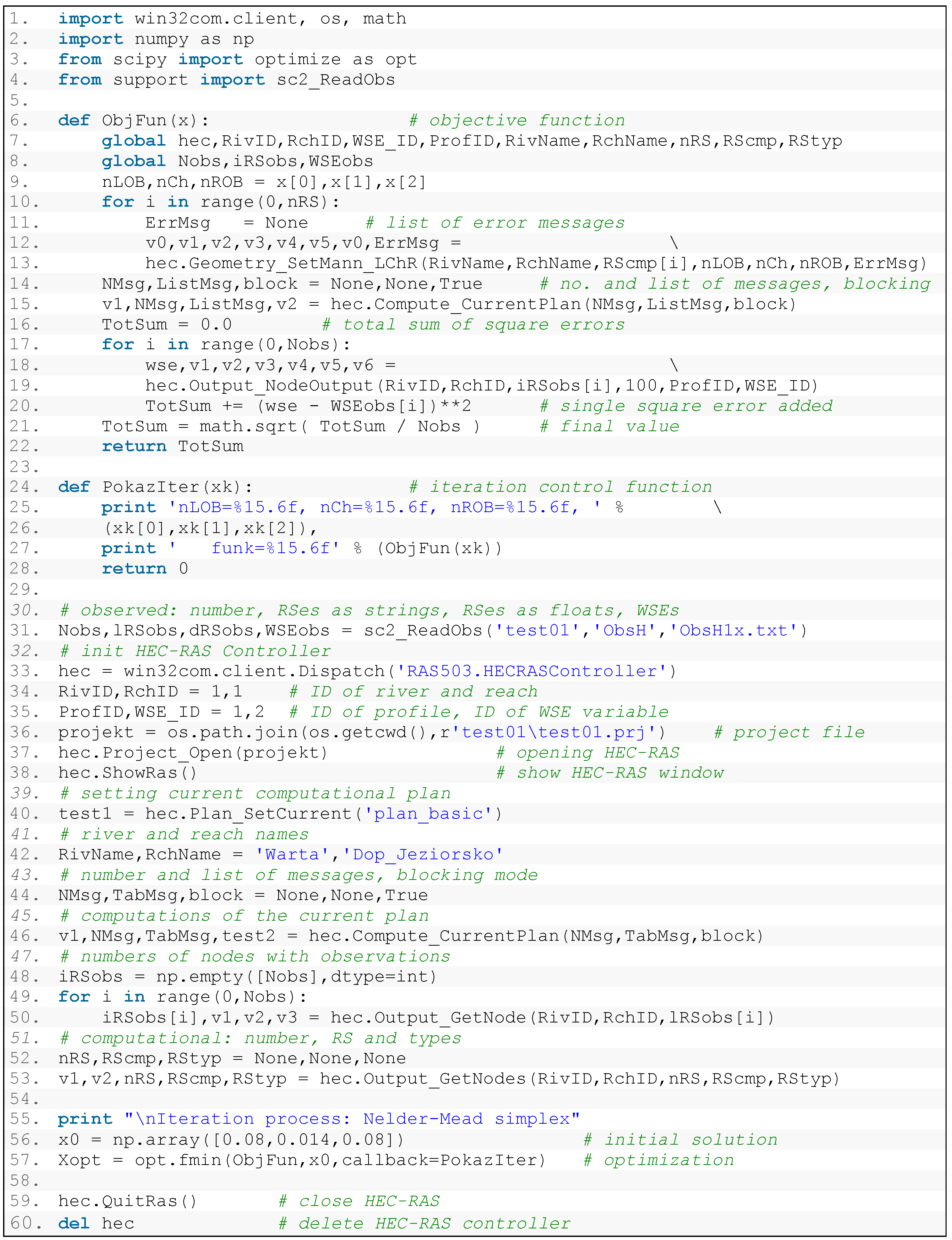
2.3. Python Scripting and Applied Modules

Python is one of the most popular programming languages today, and it is still under development. In this paper, version 2.7.12 was used. Its usefulness and popularity in many areas have been reported in References [51,52,53]. This scripting language is relatively simple for the beginner, but it is also very powerful if applied by an experienced coder. A description of this language may be found in many books or on internet websites, e.g., Downey et al. [54], Python Software Foundation [26]. Considering the problem considered here, Python has several specific advantages:

(1)

The basic language is extended by additional modules for numerical simulation and general scientific analysis, e.g., NumPy and SciPy [29,30,31].

(2)

The usefulness of Python in numerical simulations may be extended by the user with modules enabling transformation of Fortran or C routines to Python code, e.g., F2Py [32] and ctypes [33] modules.

(3)

It is possible to access COM libraries using additional modules, e.g., Pywin32 [34,35].

(4)

Python enables access to more sophisticated data structures, e.g., XML [36] and HDF5 [37].

(5)

There are Python modules integrating this language with geoprocessing software, such as ArcGIS [38] and QGIS [39].

VBA is a compiled language, which makes it faster in comparison with any scripting language in stand-alone applications. However, in the analyzed cases, the programming language is used to run an external application, HEC-RAS. Hence, the efficiency of the external application determines the efficiency of the whole concept, which reduces this advantage of VBA. The above list of Python features is the list of undoubted advantages of this scripting language over standard VBA. In some cases, the application of Python is as easy as VBA, e.g., access to COM libraries or XML data. Other elements, such as libraries for numerical computations, make Python implementation more effective. There are also features that are unique to Python, e.g., access to HDF5 data, and linking with Fortran and C. The undeniable advantage of Python is also clearly visible in the area of geoprocessing. This area is important for any hydrological or hydraulic modeling of flow and transport processes in natural water systems. As mentioned above, the former applications of VBA in older versions of ArcGIS are now replaced by modern scripting languages, such as Python [38], JavaScript [55], and R [56]. Python is the primary scripting language used in commercial Esri software, such as ArcGIS 10.x and ArcGIS Pro. This is also the only scripting language implemented in QGIS, which is the open source and cross-platform equivalent of Esri’s packages.

Several Python modules are used in this research, including: (1) Pywin32, (2) NumPy, (3) SciPy with optimization, (4) ElementTree XML API, and (5) HDF 5 for Python. The first of them, the Pywin32 module, is used to access COM objects and COM servers in Python code [34,35]. Brief descriptions of available Pywin32 packages may be found in the PythonCOM Documentation Index [35]. The part of the module win32com.client is used in this paper. To access COM objects in the presented scripts, the Dispatch function is applied.

NumPy is a well-known module including objects and tools for scientific computing [20,57]. The functions and objects from the NumPy module work faster in numerical applications than standard Python functions and variables. The reason is that the main elements of NumPy were translated from Fortran and implemented in Python. This mechanism of method transfer may be continued by the user with the F2PY package [32] or ctypes module [33]. In the present research, only the array constructors available in NumPy were applied. These are array and empty methods. The string, integer, and float element arrays were used. However, extension of some presented examples, e.g., Examples 2 and 3, enables application of one’s own methods and opens the way for more sophisticated techniques.

Another important package used here was SciPy [29,31]. The optimization part of SciPy was implemented in Example 2. The scipy.optimization module contains several optimization methods and root finding algorithms [31]. In this study, the most basic and well-known Nelder-Mead downhill simplex algorithm was used. A detailed description of it was provided by Press et al. [58].

The sediment simulation data in HEC-RAS are stored in XML format. It is a text-based markup language, derived from the Standard Generalized Markup Language. A detailed description of XML format and usage may be found in Reference [59]. To access data stored in an XML file, the ElementTree module is applied as described in References [35,60]. This package includes objects of the Element type. They are container objects designed to store hierarchical data structures, such as XML. The Element type is a cross between a list and a dictionary in Python. The module imported is xml.etree.ElementTree.

The results of the sediment simulation are stored in HDF5 format. Large sets of numerical data are easily accessed in HDF5 through the well-described hierarchy. A description of this format may be found in HDF Group [37]. To access these data the h5py module is applied [61].

2.4. General Remarks on Analyzed Examples

Three examples were tested. The first was a code of a basic simulation composed in a way that enabled comparisons with the examples presented by Goodell [20,21]. The comparison revealed the most important differences between VBA and Python, such as initialization of HECRASController, access to controller methods, handling of data and results.

The second example was the calibration of the steady flow model. Although there is a procedure for the calibration of roughness coefficients in HEC-RAS, it works only with the unsteady flow model. However, calibration of the steady flow model is useful in many cases. Additionally, the approach presented in this example could also be applied in sensitivity analysis of the model performance or probabilistic flood risk mapping. The Nelder-Mead simplex algorithm was applied to search for the proper roughness coefficients. This is routine from the optimization part of the SciPy module, namely scipy.optimize. It works for similar purposes as the AHYDRA application [24], but the optimization algorithm is applied instead of manual alteration of roughness coefficients. The code is prepared in such a way that the applied Nelder-Mead method may be replaced with any optimization algorithm, e.g., the Genetic Algorithm as proposed by Leon and Goodell [25] with MATLAB.

The objective of the third example was to automatically change sediment samples in sediment data and run a sediment simulation. Such an approach has not been found by the author in the literature to date. The sediment sample data describe the percentage of sediment fractions in a sample. In HEC-RAS, they are called gradations. This function plays the role of a model parameter. It is necessary for the calculation of the total sediment transport, as well as transport of particular fractions. However, in practical applications it should be a piece of material sampled from the river bed. Collection of sediment samples is not very common. The measurements are local and extrapolated to a region, e.g., the cross-section. Hence, such measurements are highly uncertain, which is an additional reason for presentation of Example 3. This example is very simple, but may be extended for more sophisticated cases. It requires handling of XML and HDF5 data with special Python modules. Although, the control of sediment simulation is a more complex problem, the example is focused on change of the sediment samples, because these data are accessible in the most difficult way. If the sediment fractions may be changed by the Python script, all other elements of the sediment simulation, e.g., sediment transport formula, parameters of chosen formula, method for calculation fall velocity, etc., may be changed too. Hence, the adjustment of sediment sample in the XML file is a good illustrative example of sediment data management in general.

There are two main application areas for the mechanism presented in Example 3. The first is obviously the uncertainty or sensitivity analysis of sediment transport simulation. Considering the complexity of such computations, the analysis of sensitivity is too difficult to perform in the standard manual way. However, it is necessary if the sediment transport models are going to be used for forecast purposes, which sometimes happens today. The sediment, as well as flow data, are too uncertain to neglect this problem. The second application area is related to historical data and their processing. Sometimes data collected in the past include the full longitudinal profiles, as well as cross-sections, for different moments in time. The present author had at his disposal such data for Ner river collected for 1983, 2003, and 2007 [62]. These data were collected by the company BIPROWODMEL, for the analysis of regulation requirements. They illustrate the effects of the sedimentation process along the analyzed channel. Unfortunately, the company taking measurements did not collect sediment samples at the same time. Hence, the modeling of sediment transport in the Ner river is possible only if the model is calibrated with respect to these data. There is one important aspect which should be carefully considered. The calibration should also consider other factors, such as the sediment transport formula. However, the differences in the role and structure of the factors influencing the sediment transport simulation lead to the design of separate computational processes for each factor. One such process should be searching for an optimal sediment sample or samples, with other factors kept as constants. The third example presents the powerful capabilities of Python in this area.

An example with change of data stored in ASCII files of HEC-RAS is not presented here. Such examples have been discussed by other authors [20,25] with VBA and MATLAB. In the author’s personal opinion, the handling of the ASCII files with Python is easier than with the other languages mentioned above. Hence, such an example would not bring anything new. The third and more difficult example, with XML and HDF files, may be treated as a help or guide in dealing with ASCII files. If Python enables reading and writing of information stored in such complex formats as XML and HDF5, and it is quite easy to access the data in the ASCII files, it means that the presented scripting mechanisms could be applied to manipulate all data and results of any HEC-RAS model. This is also a huge advantage of the presented approach.

2.5. Applied Rules of Coding

There are important differences between VBA and Python, which have to be discussed before the particular examples are presented. To explain them, the well-known examples given by Goodell [20,21] are quoted and compared with the devised Python code.

The first difference is declaration of variables. In Python, the variables are created dynamically during running of the program. Their type is recognized as the values that are assigned to them. The assignment operator may change this type, any time in the script. There are exceptions to these rules, e.g., special variables such as NumPy arrays. Their shape and type have to be declared before the variable is used. In VBA, dynamic creation is also available. However, it is more convenient to switch off this mechanism with the command Option Explicit at the beginning of the module. Then the variables have to be declared statically with the Dim statement.

To use the HECRASController object in the VBA code, it has to be declared as a variable [20,21]. In Python, the object is created in a similar way by calling the Dispatch function from the module win32com.client. Then all the functions and subroutines of the HEC-RAS controller are available in Python. The access is similar to the VBA calling of the HECRASController. The scheme is shown in Script 1, Script 2, Script 3 and Script 4.

In Script 1. HECobject is the HECRASController variable in the project, arguments is the list of input parameters and return_values is the list of the values we would like to get from the subroutine. The HECobject has to initialized with the Dispatch function of the win32com.client module. Although it seems to be quite simple, there is one technical problem. The subprograms in VBA and Python have different structures and different mechanisms of data exchange with the main body of the program. There are two types of arguments used by VBA subroutines. These are the “called-by-value” and “called-by-references” arguments. Exchange of information between the subprogram and the main program based on “by-value” and “by-reference” mechanisms are well known. The arguments of the first type are used only as inputs. The second calling mechanism may work as input and output. When the function construction is used, another method for output is available, i.e., the returned value of the function. Although these mechanisms are very common and are applied in many programming languages, e.g., VBA, Pascal, Fortran, C/C++, etc., the subprograms used in Python are constructed in a different way. In general, the Python subprograms are functions. The parameters set in the function head are only inputs. The output is exchanged with the outer code only by returned values of the function. It is important to indicate that the function may return a list of values and each of them can be of different type.

To adopt HECRASController methods in Python, a change in the calling is necessary. Imagine such an example: One of the subroutines determines the value of the parameter “called-by-reference”. Let this argument be x. In the case of arguments “called-by-reference”, the variable storing the output value must be created before the subroutine is run. In Python, the variable storing the None value must be created, which means the variable without a value assigned. Such a statement is equivalent to the variable declaration in VBA and other programming languages. Then the x variable is set as the argument of the subroutine and repeated as the variable in the return list, as shown in Script 2.

In more complex cases it should be noted that the return list should follow the sequence of the argument list. An example is presented in Script 3.

If the function is run, the first variable in the return list stores the original return value of the function. It is illustrated in Script 4. The variable RV used there is the return value of the function. This approach is used in all three presented examples.

The main codes presented in Script 5, Script 6, Script 7 and Script 8 consist of the main elements necessary to access capabilities of the HEC-RAS application in Python code. There are also additional codes written in support.py. They are used for support of the main scripts. The support.py file contains the subroutines for data loading from ASCII files, for handling files and directory names, etc. All these additional subroutines are subject to the coder and may be written in several ways. Hence, they are not discussed here. The additional codes are loaded to the particular scripts, if there is such a need.

3. Results and Discussion

3.1. Case Study—Model of a River Reach

Two HEC-RAS models, called model A and model B, were used to test the presented concepts. Both of them represented a short reach of the Warta river in the central part of Poland. The reach is about 10 km long. The average width and depth of the main channel are 40 m and 1.5 m, respectively. There are two bridges along the reach. The estimated mean flow in the analyzed channel was about 47.45 m³/s. This value was estimated on the basis of the hydrological data collected at the Sieradz gauge station during 1970–2013. The observed flows for the same period vary from the minimum of 15 m³/s to the maximum of 408 m³/s [63].

In both models, the number of cross-sections was 35. The average distance between cross-sections was about 300 m. The differences between the model A and model B include the geometry and configuration of flow conditions. Model A was based on the full geometry, including bridges. The flow conditions were steady with basic discharge of 120 m³/s for the whole reach. The downstream boundary condition was the simple Normal Depth with bottom slope as a parameter. This model was used for basic simulation in Example 1. It was also applied in Example 2, for the test of calibration.

In model B, the geometry was simplified. The bridges were removed, because the model was used for simulation of sediment transport with different sediment samples. Hence, the configuration of flow conditions was based on a quasi-unsteady flow module. The upstream boundary condition was Flow Series with a constant discharge of 269 m³/s. In the downstream boundary the Normal Depth was applied once again. The slope equals 0.2‰. The sediment transport intensity was calculated on the basis of the Meyer-Peter and Müller (MPM) formula. The simulation horizon was set to 4 months, with a 6-h time step. The time step guarantees necessary numerical stability and accuracy. The simulated period was rather short. In practice, the changes of the river bed due to sediment deposition and erosion are observed in longer periods, e.g., years. Such a configuration is chosen to avoid too long computational time in this illustrative example.

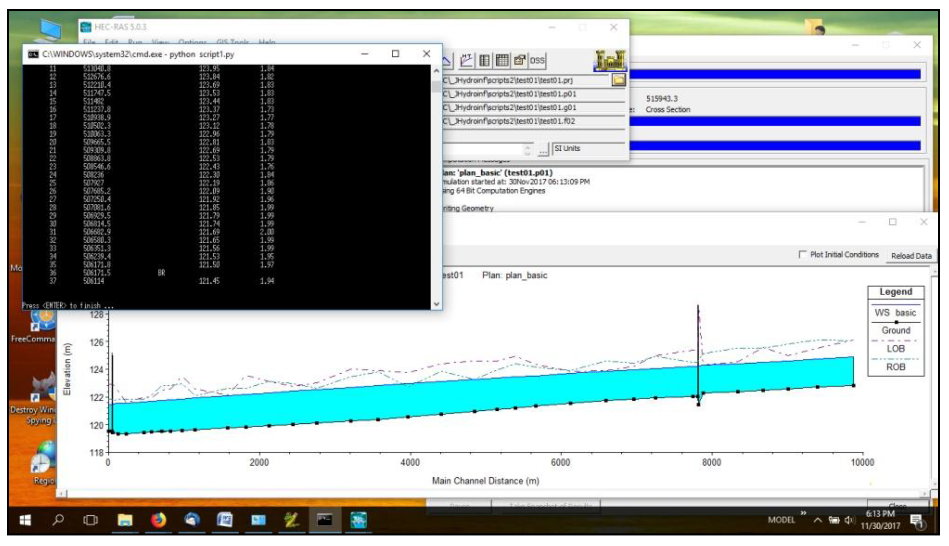
3.2. Example 1—Basic Simulation

The first example presented here was composed in a way similar to the introductory example discussed by Goodell [20,21] for the reach of Beaver Creek. In this paper, model A described above was used. The main scheme of computations is shown in Figure 1. The code of this example is presented as Script 5.

As can be seen in the first block of the diagram in Figure 1, the computations have to start with initialization of the variable, which is the HECRASController object. In the brackets, the method used for this purpose is indicated. In the second step, the HEC-RAS project is open. The name of the project is the necessary input. Then the computations are run and the results are processed in two steps. The first is reading information about computational nodes. It is done with one of the “geometric” routines of HECRASController. The second step is reading the output of computations. Then the results may be saved, displayed, or applied in another simulation.

The program presented in Script 5 includes four main steps reflecting the sequence presented in Figure 1. These are: (a) Opening HEC-RAS and loading the project (lines 9–10), (b) running the simulation (lines 12–14), (c) reading the output variables (lines 16–35), and (d) processing the output variables (line 37), e.g., displaying them on the screen. At the beginning, the necessary modules and subroutines are loaded. They are win32com.client for handling COM libraries [34,35], os for management of files and directories and numpy for numerical data. Additionally, the subroutine sc1_ShowNodes is loaded from the script support.py. It is used for displaying results.

The first step of the program is initialization of the HECRASController variable hec (line 6). The Dispatch function of the win32com.client module is applied. The HEC-RAS version used is 5.0.3. When the hec variable is created, the ShowRas and Project_Open functions may be used to open the HEC-RAS windows and load the project. Detailed descriptions of these and other functions used in the paper were provided by Goodell [20]. The next two methods of HECRASCcontroller used are Compute_CurrentPlan (line 14) and Geometry_GetNodes (line 21). The first function runs the current computational plan. The second one reads tables of River Stations, TabRS, and node types, TabNTyp. Both of them need initialization of proper arguments (lines 12 and 18). The approach presented in Code Samples 2-4 is applied. The river and reach ID numbers are also set in line 16. The variables v1, v2, and in general vX, where X is some digit, are used when the return value does not have to be stored.

The next step is reading of the output variables. It starts at line 23, with setting of the ID numbers for water stages and velocities, WSE_id and AvVel_id. Then the NumPy arrays, TabWSE, and TabVel, for storing the results are prepared (lines 24–25). The results are read in a loop over nodes (line 26–33), with calls to the function Output_NodeOutput. The values of water stages and velocities in regular cross-sections are accessed. In such nodes, the node type is an empty string (line 27).

Finally, the HEC-RAS windows is closed with QuitRas. Then the hec variable may be deleted. The last element of the code is the display of results. It is performed by sc1_ShowNode from the support module. A screenshot with the run of Example 1 and display of results is shown in Figure 2.

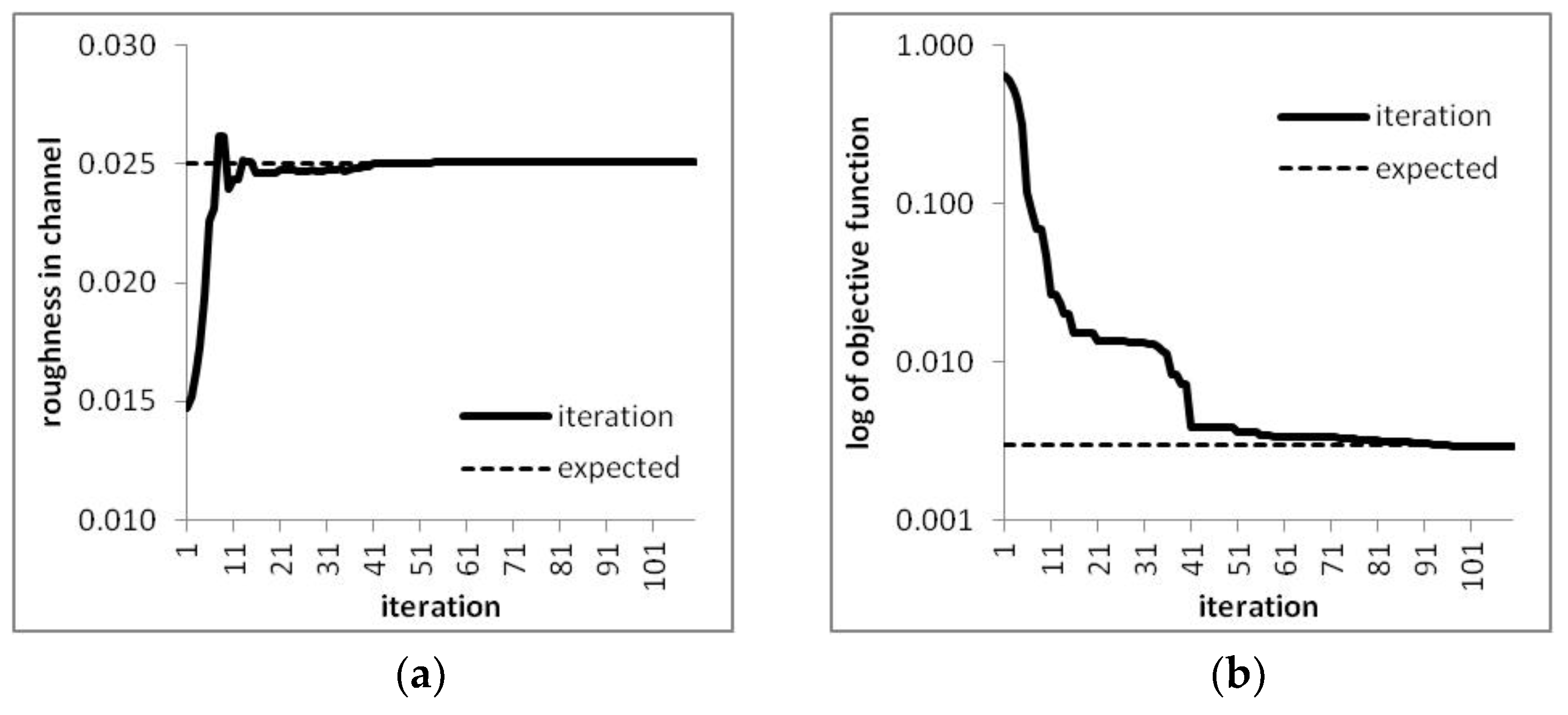
3.3. Example 2—Calibration of Roughness Coefficients

The problem of model calibration was considered. Model A described above was used here. The roughness coefficients were sought. The computations were performed in the steady mode. The calculated water surface profile should fit the imposed “observed” values. In fact, the “observed” values were calculated earlier for known roughness coefficients. Very simple distribution of their values was assumed. For the main channel along the whole reach, the value 0.025 was applied. For the left and right floodplains, one value of 0.04 was set in the same way. The purpose of the program was to find the set of optimal coefficients. It was assumed that only three values were necessary. Hence, the dimension of the problem was relatively small, but the generality of this solution is not lost.

The “observed” values were determined for each cross-section along the reach. However, they were applied with different frequencies in the search algorithm. It means that only some values were selected, and the simulated water surface was fitted only in the selected cross-sections. Hence, the objective function is as follows:

$$F\left(x\right)=\sqrt{\frac{1}{N}{\displaystyle \sum }_{i=1}^N{\left(WS{E}_i^{\left(c\right)}-WS{E}_i^{\left(o\right)}\right)}^2}$$

(5)

In the above formula, N is number of observations, $WS{E}_i^{\left(c\right)}$ is the computed water surface elevation, and $WS{E}_i^{\left(o\right)}$ is the “observed” one determined in the same i-th cross-section. This function should be minimized to find the optimal set of roughness coefficients x, where x = [n_LOB, n_Ch, n_ROB] for the left floodplain, the main channel, and the right floodplain, respectively.

The algorithm for calculation of the objective function is presented in Figure 3. It starts with processing of the input parameters. At this step, the optimization variable is transformed into computational roughness coefficients. Then the coefficients are set in all model cross-sections. This step requires access to the global variable representing the object of the HECRASController. The next elements of the algorithm are similar to the operations presented in Figure 1. The computations start and the results are read. In both these steps, the HECRASController object is processed. To read the results properly, identification of the nodes where referenced or “observed” values of the water surfaces are located is necessary. This information is taken from another global variable. Then the calculated and referenced water surface elevations are used to determine the final value of the objective function according to Equation (5). The reference water surfaces are also stored in the global variable.

The main elements of the computations in this example are shown in Figure 4. The computational process starts with initialization of the HECRASController object. Then the HEC-RAS variable is used for opening of the HEC-RAS project, setting the current computational plan and running preliminary computations. These steps are necessary to compare the information about the reference nodes and values with the structure of the computational model. For this purpose, the project name and the reference values must be loaded. After these steps, the object of the HECRASController is ready and the numbers of computational nodes for comparisons with reference nodes are known. After loading of the initial estimate, which is the set of preliminary roughness coefficients, the optimization process starts. It uses the objective function presented in Figure 3.

The starting point is an arbitrarily chosen set of roughness coefficients. The values chosen were 0.08 for the left floodplain, 0.014 for the main channel, and 0.08 for the right floodplain.

In Script 6, such modules as win32com.client, os, math, numpy and scipy.optimize are necessary. They are loaded at the beginning of the script. The function for reading the “observed” values is also loaded from the support module.

Script 6 includes two functions. The first one plays the role of an objective function and is called ObjFun. It is an argument of the optimization algorithm. Its structure is discussed below. The second one, PokazIter, is used by the same algorithm to display results of the single iteration.

The main body of the script starts with the reading of “observed” values in line 31. They are stored as lists of River Stations, lRSobs and dRSobs, and a list of water surface elevations, WSEobs. Then the HEC-RAS variable, hec, is created (line 33). Before the project is opened (line 37), the HEC-RAS window is displayed (line 38) and the current plan is set (line 40), the project constants are set (line 34–35). They are the river and reach IDs, RivID and RchID, profile number, ProfID, and ID of the output variable storing water surfaces, WSE_ID. The names of the river and the reach, RivName and RchName (line 42), are also hard-coded in the script, though they could be read using the methods of the HEC-RAS controller.

The first computations are run in line 46. The necessary variables are prepared earlier (line 44). The only purpose of these preliminary computations is to check the numbers of nodes, at which the “observed” values are determined. The function Output_GetNode is used for this purpose. The important argument of the function is River Station, inserted as a string, lRSobs[i]. The numbers of the “observed” nodes are stored as NumPy array of integers, iRSobs.

The computational nodes, RScmp, and their types, RStyp, are also read from the results of the preliminary computations.

The optimization process with Nelder-Mead simplex starts at line 57. A detailed description of this function may be found at SciPy.org [28]. Before this the initial guess, x0, is prepared as a NumPy array. The main argument of the optimization algorithm is the objective function, ObjFun. It is defined as a separate function (lines 6–22).

The basic argument of the objective function is the set of searched parameters x. It is a 3-element NumPy array. At the very beginning, the parameters x are assigned to the variables, representing roughness coefficients nLOB, nCh, nROB. The roughness coefficients are set for any cross-section of the HEC-RAS project in a loop over nodes with the function Geometry_SetMann_LChR. The subsequent steps are running of the computations (line 15) and reading the results (line 19) in the loop over nodes (lines 17–20). These processes are performed with the HECRASController functions Compute_CurrentPlan and Output_NodeOutput. Both of them were used in the previous example. The difference between the computed, wse, and “observed”, WSEobs[i], water surfaces in a single node is calculated in line 20. The final value of the objective function is determined beyond the loop, in line 21. When the optimization process stops, the HEC-RAS window is closed and the controller variable is deleted.

The results obtained in Example 2 are shown in Figure 5. Part (a) presents the convergence of the channel roughness during the run. Part (b) shows changes of the objective function (5) during the computations.

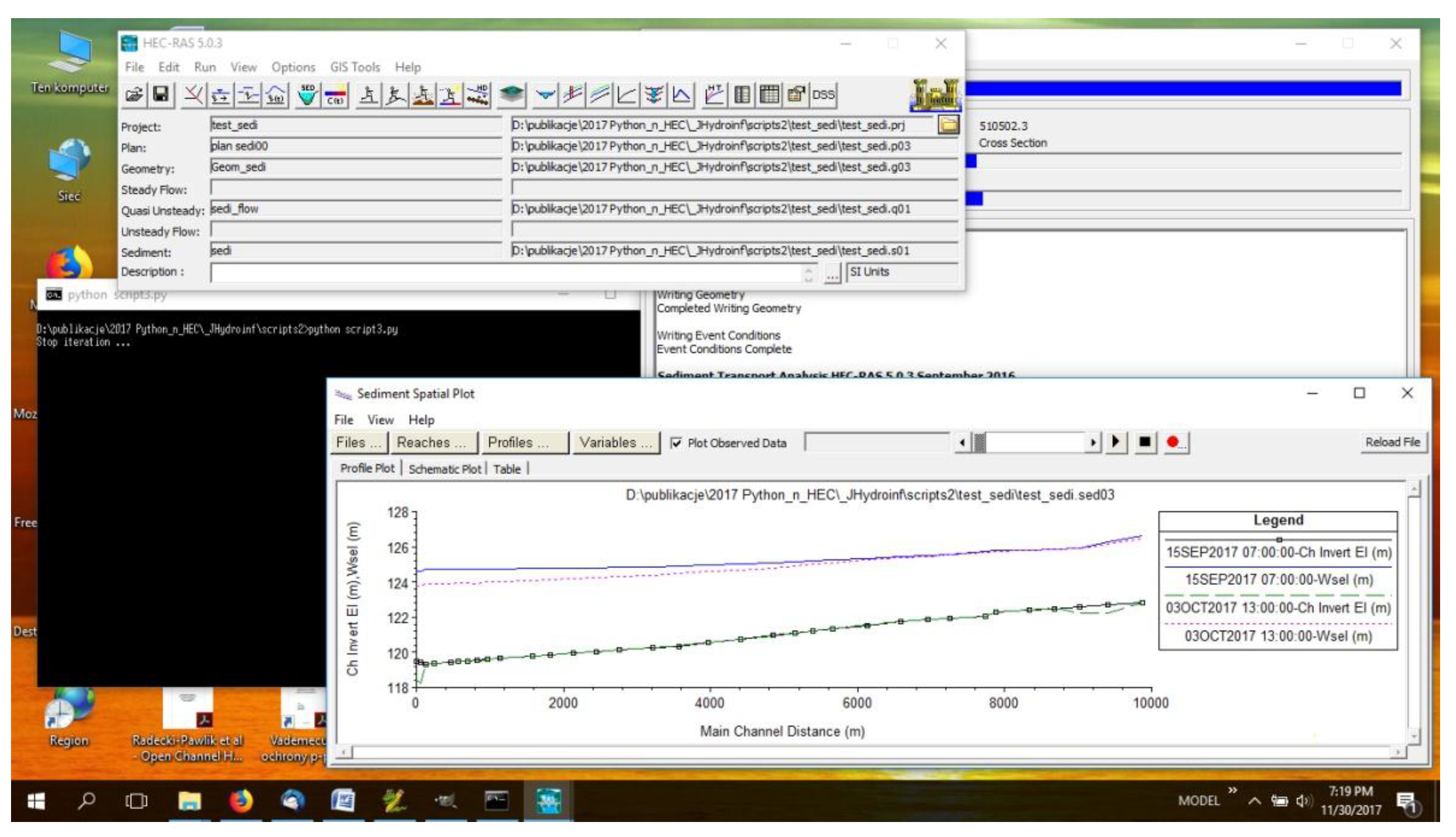
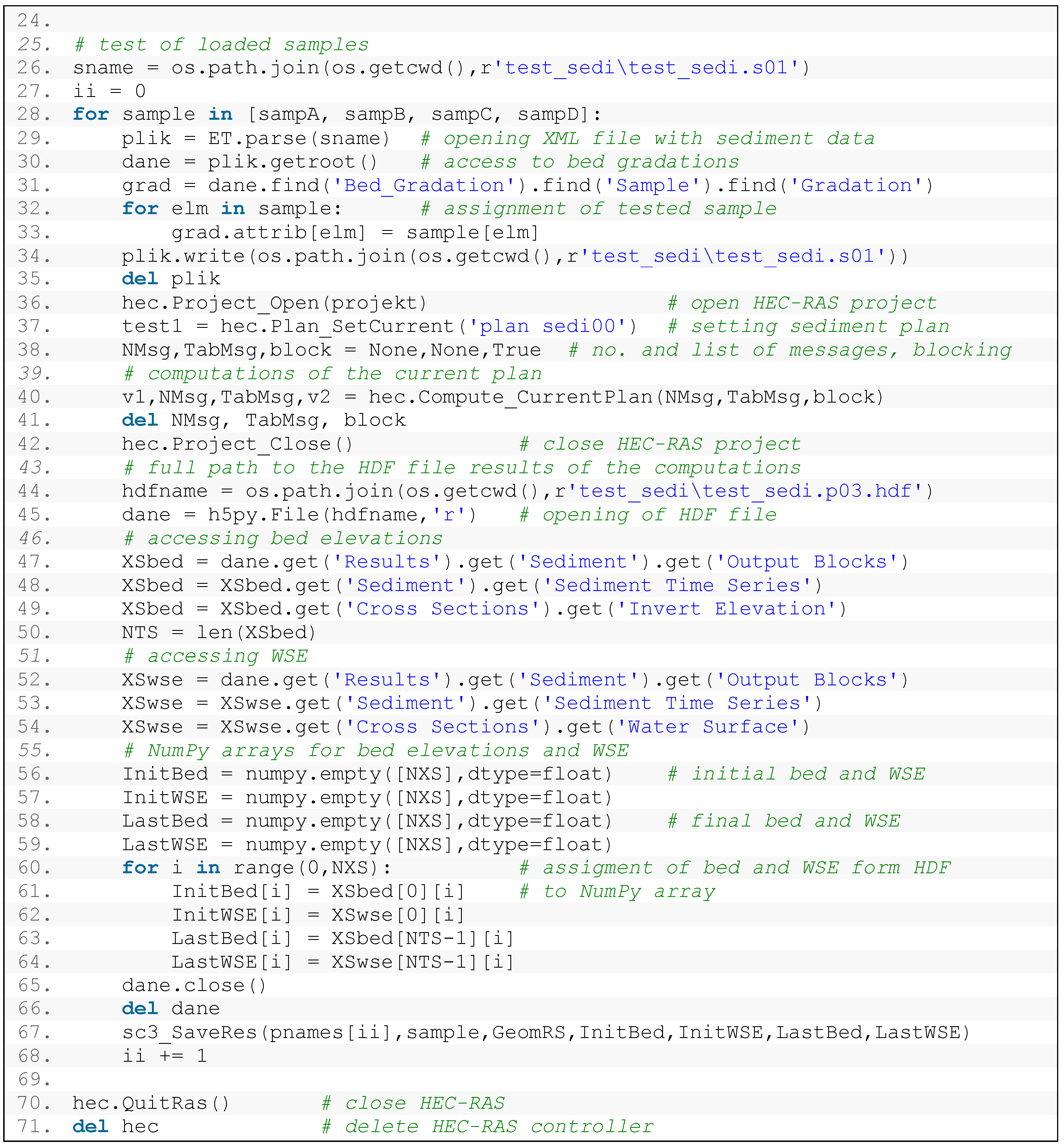
3.4. Example 3—Control of Sediment Simulation

The purpose of this example is to show that sediment simulation in HEC-RAS may be run several times for different sediment samples. Model B described above is used in this case. The samples are changed automatically by the Python code. The HEC-RAS sediment data file has the XML format. Hence, the xml.etree.ElementTree module [36] is necessary to read and handle data. The results are then read from HDF files with the methods available in the h5py module [59]. The code in this example is very simple. However, the methods presented here may be extended and applied in a more sophisticated code, e.g., calibration of the sediment routing algorithm, analysis of sediment simulation uncertainty, or assessment of flow regime changes caused by sediments.

The third example is too long to present all lines of code in one script. Hence, it is split into Script 7 and Script 8. There are four files with data and results managed in this script. The first is the file storing the tested sediment samples. The format of this file is arbitrary and it will not be discussed here. The only requirement is that the loaded sediment samples should have a form similar to those stored in HEC-RAS. Three other files are more specific. They are the XML file with HEC-RAS sediment data, the HDF file with geometric data, and the HDF file with the results.

An example of the sediment data file is shown in Figure 6a. It is presented in the XML Viewer. It has a structure similar to a tree. The groups include subgroups and so on. A description of the XML format can be found in the document prepared by the Python Software Foundation [36]. The group with bed gradation is opened in the XML Viewer. The name of the file and the full hierarchy to access these data are shown in

Table 1. Loading data and results from XML and HDF files: type of data, type of file, access hierarchy.

Data	File		Access Hierarchy
	Type	Name
sediment sample	XML	test_sedi.s01	Data\Bed_Gradation\Sample\Gradation
River Stations	HDF	test_sedi.g03.hdf	Geometry\Cross Sections\River Stations
bed elevations	HDF	test_sedi.p03.hdf	Results\Sediment\Output Blocks\Sediment\Sediment Time Series\Cross Sections\Invert Elevation
water surface elevations	HDF	test_sedi.p03.hdf	Results\Sediment\Output Blocks\Sediment\Sediment Time Series\Cross Sections\Water Surface

. Particular gradations are stored as the group attribute. This attribute is a dictionary, where the class symbols ‘GC1’, ‘GC2’, etc. reflect the gradation in the format ‘%Finer’. Every XML file is an ASCII file, and it may be opened in Windows Notepad.

The HDF files may be opened in HDFViewer, as presented in Figure 6b. These are simulation results files in binary format. It is not possible to use Notepad to open them, but the HDF also has a structure similar to a tree with successive branches. Two elements are read from the opened HDF file. These are (a) the invert elevations and (b) the water surface elevations. The first is shown in Figure 6b. The hierarchy to access these data is also presented in Table 1.

The flow chart of the main computations in this example is shown in Figure 7. The main element is a loop over sediment samples. Before the loop starts, the HECRASController object has to be initialized and the name of the project has to be loaded. If the HEC-RAS variable is ready, the information about computational nodes may be read from the HDF5 file storing geometry data. Before the loop starts, the sediment samples have to be loaded to the script. The first step in the loop is access to the XML file with sediment data. The grain fractions are written and the XML file is closed. Then the project can be opened, because any change of the sediment data in the XML file is noticed by the HEC-RAS project only in the phase of the data loading. Further changes of the data in files stored on the disk do not affect the project. Then the computations start and the results are read from the HDF5 file. At the end of each step, the bed elevations and positions of the computational nodes are written to the separate ASCII file, which enables preparation of the bed profiles.

The program presented in Script 7 and Script 8 starts with import of necessary modules (lines 1–4). The modules win32com.client, os, numpy are also applied in the previous examples. The new elements are xml.etree.ElementTree and h5py. The first one is loaded as ET, and it is used for handling the XML documents. The second one is used for reading of data and results from HDF files. Two functions are loaded from the support module. They are sc3_LoadPrb for loading sediment samples, and sc3_SaveRes for saving results in ASCII files. For the sake of simplicity, no local functions are defined.

The first command is reading of the sediment samples for tests (lines 7–8). The samples are stored as dictionaries sampA, sampB, sampC, and sampD. Their items are composed of sediment class denotation in the format ‘GC#’ and weighted gradation as ‘%Finer’. The keys of the dictionary should be the same as those used in the HEC-RAS and XML files with sediment data. The first element of the return list, pnames, is the table with samples’ names.

The HECRASController starts at line 11. The HEC-RAS window is opened (line 13) and the full path of the project file is set, but the project is not loaded. Every change in the data requires reloading of the project. Hence, the project is loaded later.

The HDF file including geometry data is opened first (line 16). The link to the River Stations is created (line 18) with the get method of the h5py module. Then the NumPy array for storing these data is prepared (line 19). The data are assigned as value-by-value in a loop over nodes. Then the first HDF file is closed (line 22). The important element taken from the River Station array is the number of cross-sections NXS (line 23). The rest of the commands are shown in Script 8.

The longest part of the script is the loop over tested samples (lines 28–68). At the beginning of each step, the XML file with sediment data is opened (line 29). Then the link to bed gradation grad is created. In the internal loop (lines 32–33) over items of the sample, the bed gradations in the XML file are replaced with bed gradations of the current sample (line 33). Then the file is saved (line 34) and closed by deleting the variable representing this file. At this moment the XML file with sediment data is ready. The HEC-RAS project is opened (line 36) and the computational plan is set properly (line 37). After the current plan is computed (line 40), the project is closed (line 42). The last file of the current iteration is accessed (line 45). This is the HDF file with results of the computations (Table 1). Two elements are read from this file: Bed elevations and water surface elevations. These results are stored as list of successive time steps. Each time step is a list of values stored for each cross-section. The links to the bed and water surface elevations, XSbed and XSwse, are created in lines 47–49 and 52–54. The number of time steps is assigned to the variable NTS.

The NumPy arrays for storing the initial and final bed and surface elevations are created in lines 56–59. The results are assigned to them in another internal loop (lines 60–64) over cross-sections. Later, the HDF file is closed (lines 65–66). Finally, the results are saved in a file specific for each iteration, whose name is the name of the sample. At the end of the script, HEC-RAS is closed and the variable hec is deleted.

The sediment simulation running from the Python script is shown in Figure 8. The display of typical output for such simulation is also shown in the screenshot. The sieve curves of tested sediment samples are plotted in Figure 9a. The variability of assumed sieve curves is typical for a lowland river. The differences in the content of bed sediments are relatively small. However, more complex examples may also be tested in the same way. Figure 9b shows the results of the simulation as bed changes in the selected cross-sections. Considering the time horizon of the simulation, which is 4 months, the bed changes from −20 cm to +60 cm seem to be quite significant. The reason is the relatively huge discharge of 269 m³/s, kept constant during the whole simulation. The differences between the changes of bed elevations vary from a few to 10 cm. If we compare this result with the range of changes, which is about 80 cm, it transpires that the differences between consecutive simulations are up to 12.5% for a very short simulation period. This stresses the importance of the sediment sample variability for the sensitivity of the sediment transport model.

4. Conclusions

The examples presented in this paper explain the techniques necessary to control HEC-RAS computations with Python. The main element of the presented methods is the application of Python module Pywin32 for handling COM libraries. This module was used in all three examples. The comparison of the code developed for Example 1, with basic examples discussed by Goodell [20,21] and Leon and Goodell [25], illustrates the ease of Python application for handling HECRASController. The use of Python is not more difficult than VBA or MATLAB. Additionally, Example 1 presents a more general approach for application of Python for control of HEC-RAS computations than described in previous papers [40,41]. This example explains how to control any version of HEC-RAS, including the future developments. It also opens doors for further extension of HECRASController capabilities. Possible further extensions were shown in Examples 2 and 3.

The second example presented the application of HECRASController and Python specific modules, for the automatic calibration of the HEC-RAS model. The roughness coefficients were determined by the optimization method from the SciPy module. This approach was similar to that presented by Leon and Goodell [25], where the Genetic Algorithm from the MATLAB toolbox was applied for control of gate operation. Example 2 was also a more advanced approach for determination of roughness coefficients than that presented in the AHYDRA package [24]. Further development of the techniques presented in Example 2, could focus on application of a faster and/or more sophisticated optimization method than the Nelder-Mead simplex. It is also possible to develop a more general Python module for automatic calibration of HEC-RAS, on the basis of the concept presented here. Example 2 may also be improved by preparation of a user optimization algorithm. It could be implemented in Fortran, which is very fast and aimed at numerical computations, and then it could be translated to Python with the F2PY or ctypes modules.

Example 2 presented the linkage of HEC-RAS computations with numerical routines available in specific Python modules, NumPy and SciPy. The number of useful routines in SciPy is greater than those presented. Other extensions and HEC-RAS applications are also possible. The elements available in NumPy are also very useful for storing and handling of computational results. These features of Python are undoubted advantages of Python over standard VBA.

Example 3 illustrated an extension of HECRASController capabilities to control sediment simulation. To the best of the author’s knowledge, such an approach or a similar one has not been tested yet. These examples presented a real advantage of Python, owing to the access to very complex data formats, XML and HDF5. The Python modules enabling such access are ElementTree and H5PY, respectively. There are several applications of the presented approach. The most basic is sensitivity analysis of sediment transport simulation. Another possible use is calibration of the sediment model on the basis of the historical data. These two application areas are discussed in the text. Other applications are also possible in the area of water management. Examples may be the impact of sediment deposition on flood hazard, prediction of morphodynamic changes in the river after regulation, etc. The uncertainty of sediment transport modeling may also be estimated with the techniques used in Example 3.

The illustrated capabilities of Python are not the only advantages of this scripting language over specific VBA applications. Another is access to geoprocessing tools, such as ArcGIS and QGIS. It makes integration of Python with HEC-RAS more necessary. Not only are VBA capabilities too poor to compete with Python in this area; more dedicated numerical software such as MATLAB does not have such broad capabilities for geoprocessing.

Application of Python for control of hydrodynamic simulations with HEC-RAS opens new opportunities in such areas as water management, river engineering, and flood risk management. Good opportunities are available by access to more different data formats from simple text files to more complex XML and HDF5. A huge advantage is the linking of HEC-RAS with other software, such as numerical routines or geoprocessing. More advanced future applications are also possible.

References

1. Kachiashvili, K.J.; Melikdzhanian, D.I. Software realization problems of mathematical models of pollutants transport in rivers. Adv. Eng. Softw. 2009, 40, 1063–1073. [Google Scholar] [CrossRef]
2. Zischg, A.P.; Mosimann, M.; Bernet, D.B.; Röthlisberger, V. Validation of 2D flood models with insurance claims. J. Hydrol. 2018, 557, 350–361. [Google Scholar] [CrossRef]
3. Pinar, E.; Paydas, K.; Seckin, G.; Akilli, H.; Sahin, B.; Cobaner, M.; Kocaman, S.; Akar, M.A. Artificial neural network approaches for prediction of backwater through arched bridge constrictions. Adv. Eng. Softw. 2010, 41, 627–635. [Google Scholar] [CrossRef]
4. Shen, D.Y.; Jia, Y.; Altinakar, M.; Bingner, R.L. GIS-based channel flow and sediment transport simulation using CCHE1D coupled with AnnAGNPS. J. Hydraul. Res. 2016, 54, 567–574. [Google Scholar] [CrossRef]
5. Gibson, S.; Sánchez, A.; Piper, S.; Brunner, G. New One-Dimensional Sediment Features in HEC-RAS 5.0 and 5.1. In Proceedings of the World Environmental and Water Resources Congress 2017, Sacramento, CA, USA, 21–25 May 2017; pp. 192–206. [Google Scholar]
6. Horritta, M.S.; Bates, P.D. Evaluation of 1D and 2D numerical models for predicting river flood inundation. J. Hydrol. 2002, 268, 87–99. [Google Scholar] [CrossRef]
7. Rodriguez, L.B.; Cello, P.A.; Vionnet, C.A.; Goodrich, D. Fully conservative coupling of HEC-RAS with MODFLOW to simulate stream–aquifer interactions in a drainage basin. J. Hydrol. 2008, 353, 129–142. [Google Scholar] [CrossRef]
8. Drake, J.; Bradford, A.; Joy, D. Application of HEC-RAS 4.0 temperature model to estimate groundwater contributions to Swan Creek, Ontario, Canada. J. Hydrol. 2010, 389, 390–398. [Google Scholar] [CrossRef]
9. Brunner, G.W. HEC-RAS River Analysis System Hydraulic Reference Manual; US Army Corps of Engineers; Report No. CPD-69; Hydrologic Engineering Center (HEC): Davis, CA, USA, 2016. [Google Scholar]
10. DHI. MIKE 11—A Modeling System for Rivers and Channels User Guide, DHI Software. 2003. Available online: https://www.tu-braunschweig.de/Medien-DB/geooekologie/mike11usersmanual.pdf (accessed on 10 May 2018).
11. Deltares. SOBEK User Manual, Delft, The Netherlands, 2018. Available online: https://content.oss.deltares.nl/delft3d/manuals/SOBEK_User_Manual.pdf (accessed on 10 May 2018).
12. Caponi, F.; Ehrbar, D.; Facchini, M.; Kammerer, S.; Koch, A.; Peter, S.; Vonwiller, L. BASEMENT System Manuals–Reference Manual, VAW–ETH, Zurich, 2017. Available online: http://people.ee.ethz.ch/~basement/baseweb/download/documentation/BMdoc-Reference-Manual-v2-7.pdf (accessed on 10 May 2018).
13. Greimann, B.; Huang, J.V. SRH-1D 4.0 User’s Manual; Bureau of Reclamation: Denver, CO, USA, 2018. Available online: https://www.usbr.gov/tsc/techreferences/computer%20software/models/srh1d/index.html (accessed on 10 May 2018).
14. Pappenberger, F.; Beven, K.; Horritt, M.; Blazkova, S. Uncertainty in the calibration of effective roughness parameters in HEC-RAS using inundation and downstream level observations. J. Hydrol. 2005, 302, 46–69. [Google Scholar] [CrossRef]
15. Vansteenkiste, T.; Tavakoli, M.; Ntegeka, V.; De Smedt, F.; Batelaan, O.; Pereira, F.; Willems, P. Intercomparison of hydrological model structures and calibration approaches in climate scenario impact projections. J. Hydrol. 2014, 519, 743–755. [Google Scholar] [CrossRef]
16. Shrestha, B.; Cochrane, T.A.; Caruso, B.S.; Arias, M.E.; Piman, T. Uncertainty in flow and sediment projections due to future climate scenarios for the 3S Rivers in the Mekong Basin. J. Hydrol. 2016, 540, 1088–1104. [Google Scholar] [CrossRef]
17. Guo, A.; Chang, J.; Wang, Y.; Huang, Q.; Zhou, S. Flood risk analysis for flood control and sediment transportation in sandy regions: A case study in the Loess Plateau, China. J. Hydrol. 2018, 560, 39–55. [Google Scholar] [CrossRef]
18. Dimitriadis, P.; Tegos, A.; Oikonomou, A.; Pagana, V.; Koukouvinos, A.; Mamassis, N.; Koutsoyiannis, D.; Efstratiadis, A. Comparative evaluation of 1D and quasi-2D hydraulic models based on benchmark and real-world applications for uncertainty assessment in flood mapping. J. Hydrol. 2016, 534, 478–492. [Google Scholar] [CrossRef]
19. Afshari, S.; Tavakoly, A.A.; Rajib, M.A.; Zheng, X.; Follum, M.L.; Omranian, E.; Fekete, B.M. Comparison of new generation low-complexity flood inundation mapping tools with a hydrodynamic model. J. Hydrol. 2018, 556, 539–556. [Google Scholar] [CrossRef]
20. Goodell, C. Breaking HEC-RAS Code. A User’s Guide to Automating HEC-RAS; h2ls: Portland, OR, USA, 2014. [Google Scholar]
21. Goodell, C. Automating HEC-RAS, The RAS Solution. 2014. Available online: http://hecrasmodel.blogspot.com/2014/10/automating-hec-ras.html (accessed on 20 November 2017).
22. Yang, T.-H.; Wang, Y.-C.; Tsung, S.-C.; Guo, W.-D. Applying micro-genetic algorithm in the one-dimensional unsteady hydraulic model for parameter optimization. J. Hydroinform. 2014, 16, 772–783. [Google Scholar] [CrossRef]
23. Lacasta, A.; Morales-Hernández, M.; Burguete, J.; Brufau, P.; García-Navarro, P. Calibration of the 1D shallow water equations: A comparison of Monte Carlo and gradient-based optimization methods. J. Hydroinform. 2017, 19, 282–298. [Google Scholar] [CrossRef]
24. Vladyman. Automating Hydraulic Analysis (AHYDRA) v. 1.0. 2011. Available online: http://ahydra.yolasite.com/ (accessed on 7 November 2017).
25. Leon, A.S.; Goodell, C. Controlling HEC-RAS using MATLAB. Environ. Model. Softw. 2016, 84, 339–348. [Google Scholar] [CrossRef] [Green Version]
26. Python Software Foundation. Python 2.7.14 Documentation. 2017. Available online: https://docs.python.org/2/index.html (accessed on 8 November 2017).
27. Galiano, V.; Migallón, H.; Migallón, V.; Penadés, J. PyPnetCDF: A high level framework for parallel access to netCDF files. Adv. Eng. Softw. 2010, 41, 92–98. [Google Scholar] [CrossRef]
28. Patzák, B.; Rypl, D.; Kruis, J. MuPIF—A distributed multi-physics integration tool. Adv. Eng. Softw. 2013, 60–61, 89–97. [Google Scholar] [CrossRef]
29. SciPy Community SciPy Reference Guide. 2017. Available online: https://docs.scipy.org/doc/scipy/reference/ (accessed on 24 November 2017).
30. SciPy.org NumPy. 2017. Available online: http://www.numpy.org/ (accessed on 8 November 2017).
31. SciPy.org Optimization and Root Finding (scipy.optimize). 2017. Available online: https://docs.scipy.org/doc/scipy/reference/optimize.html (accessed on 8 November 2017).
32. SciPy.org F2PY Users Guide and Reference Manual. 2017. Available online: https://docs.scipy.org/doc/numpy-dev/f2py/ (accessed on 24 November 2017).
33. Python 2.7.15 Documentation. Available online: https://docs.python.org/2/index.html (accessed on 11 September 2018).
34. Hammond, M.; Robinson, A. Python Programming on Win32; O’Reilly Media, Inc.: Sebastopol, CA, USA, 2000. [Google Scholar]
35. PythonCOM Documentation Index Python and COM. Blowing the Rest Away! 2017. Available online: http://docs.activestate.com/activepython/2.4/pywin32/html/com/win32com/HTML/docindex.html (accessed on 8 November 2017).
36. Python Software Foundation. The ElementTree XML API, in Python Software Foundation. 2017. Available online: https://docs.python.org/2/library/xml.etree.elementtree.html (accessed on 8 November 2017).
37. HDF Group. High Level Introduction to HDF5. 2016. Available online: https://support.hdfgroup.org/HDF5/Tutor/HDF5Intro.pdf (accessed on 24 November 2017).
38. Zandbergen, P.A. Python Scripting for ArcGIS; Esri Press: Redlands, CA, USA, 2013. [Google Scholar]
39. QGIS Project PyQGIS Developer Cookbook Release 2.18. 2017. Available online: http://docs.qgis.org/2.18/pdf/en/QGIS-2.18-PyQGISDeveloperCookbook-en.pdf (accessed on 26 November 2017).
40. Peña-Castellanos, G. PyRAS—Python for River AnalysiS; MIT License. 2015. Available online: https://pypi.python.org/pypi/PyRAS/ (accessed on 7 November 2017).
41. Vimal, S. PyFloods. Python Module for Floods. 2015. Available online: https://github.com/solomonvimal/PyFloods (accessed on 7 November 2017).
42. Chow, V.T. Open Channel Hydraulics; McGraw-Hill: New York, NY, USA, 1959. [Google Scholar]
43. Henderson, F.M. Open Channel Flow. Macmillan Series in Civil Engineering; Macmillan Company: New York, NY, USA, 1966. [Google Scholar]
44. Abbott, M.B.; Minns, A.W. Computational Hydraulics; Ashgate Publishing: Farnham, UK, 1979. [Google Scholar]
45. Cunge, J.A.; Holly, F.M.; Verwey, A. Practical Aspects of Computational River Hydraulics; Pitman Advanced Publishing Program: Boston, MA, USA, 1980. [Google Scholar]
46. Wu, W. Computational River Dynamics; Taylor & Francis Group: London, UK, 2007. [Google Scholar]
47. Szymkiewicz, R. Numerical Modeling in Open Channel Hydraulics. In Water Science and Technology Library; Springer: Dordrecht, The Netherlands, 2010; Volume 83. [Google Scholar]
48. Leonard, B.P. A Stable and Accurate Convective Modelling Procedure Based on Quadratic Upstream Interpolation. In Computer Methods in Applied Mechanics and Engineering; North-Holland Publishing Company: Amsterdam, The Netherlands, 1979; Volume 19, pp. 59–98. [Google Scholar]
49. Brunner, G.W. HEC-RAS River Analysis System User’s Manual Version 5.0; US Army Corps of Engineers; Report No. CPD-68; Hydrologic Engineering Center (HEC): Davis, CA, USA, 2016. [Google Scholar]
50. Green, J.; Bullen, S.; Bovey, R.; Alexander, M. Excel 2007 VBA Programmer’s Reference; Wiley Publishing, Inc.: Indianapolis, IN, USA, 2007. [Google Scholar]
51. Sandler, R. The 14 Most Popular Programming Languages, According to a Study of 100,000 Developers. Buisness Insider, 2018. Available online: https://www.businessinsider.com/14-most-popular-programming-languages-stack-overflow-developer-survey-2018-4 (accessed on 8 September 2018).
52. Putano, B. Most Popular and Influential Programming Languages of 2018, Stackify. 2017. Available online: https://stackify.com/popular-programming-languages-2018/ (accessed on 8 September 2018).
53. Petkov, A. Here Are the Best Programming Languages to Learn in 2018. freeCodeCamp.org, 2018. Available online: https://medium.freecodecamp.org/best-programming-languages-to-learn-in-2018-ultimate-guide-bfc93e615b35 (accessed on 8 September 2018).
54. Downey, A.; Elkner, J.; Meyers, C. How to Think Like a Computer Scientist. Learning with Python; Green Tea Press: Wellesley, MA, USA, 2002; Available online: http://www.greenteapress.com/thinkpython/thinkCSpy.pdf (accessed on 8 November 2017).
55. Rubalcava, R. Introducing ArcGIS API 4 for JavaScript: Turn Awesome Maps into Awesome Apps; Apress: New York, NY, USA, 2017. [Google Scholar]
56. Pobuda, M. Using the R-ArcGIS Bridge: The Arcgisbinding Package. Available online: https://r-arcgis.github.io/assets/arcgisbinding-vignette.html (accessed on 11 September 2018).
57. Tutorials Point NumPy. Tutorials Point (I) Pvt. Ltd., 2016. Available online: https://www.tutorialspoint.com/numpy/ (accessed on 24 November 2017).
58. Press, W.H.; Teukolsky, S.A.; Vetterling, W.T.; Flannery, B.P. Numerical Recipes in Fortran 77: The Art of Scientific Computing, Volume 1 of Fortran Numerical Recipes. Second Edition, University of Cambridge. 1992. Available online: http://numerical.recipes/oldverswitcher.html (accessed on 24 November 2017).
59. Tutorials Point XML. Tutorials Point (I) Pvt. Ltd., 2017. Available online: https://www.tutorialspoint.com/xml/ (accessed on 24 November 2017).
60. Lundh, F. Elements and Element Trees. 2007. Available online: http://effbot.org/zone/element.htm (accessed on 24 November 2017).
61. Collette, A. h5py Documentation. 2017. Available online: http://docs.h5py.org/en/latest/ (accessed on 8 November 2017).
62. Dysarz, T.; Szałkiewicz, E.; Wicher-Dysarz, J. Long-term impact of sediment deposition and erosion on water surface profiles in the Ner river. Water 2017, 9, 168. [Google Scholar] [CrossRef]
63. Wicher-Dysarz, J.; Dysarz, T. Analiza procesu akumulacji rumowiska w górnej części zbiornika Jeziorsko. Gospodarka Wodna 2016, 9, 292–298. (In Polish) [Google Scholar]
Script 1. Code sample 1. Initialization of HEC-RAS object and schematic use of its methods.
Water 10 01382 sch001
Script 2. Code sample 2. Initialization of the HEC-RAS object and use of its methods requiring passing of the argument by reference.
Water 10 01382 sch002
Script 3. Code sample 3. Passing the arguments by reference to the method of the HEC-RAS object playing the role of a subroutine.
Water 10 01382 sch003
Script 4. Code sample 4. Passing the arguments by reference to the method of the HEC-RAS object playing the role of a function with one return value.
Water 10 01382 sch004
Figure 1. Main elements of computations in Example 1.
Water 10 01382 g001
Script 5. Example 1. Calculation of a single water profile.
Water 10 01382 sch005
Figure 2. Run of Example 1 and display of results.
Water 10 01382 g002
Figure 3. Algorithm for calculation of objective function values.
Water 10 01382 g003
Figure 4. Main computational elements of Example 2.
Water 10 01382 g004
Script 6. Example 2. Calibration of HEC-RAS steady flow model.
Water 10 01382 sch006
Figure 5. Results of Example 2: (a) convergence of channel roughness coefficient, (b) convergence of objective function.
Water 10 01382 g005
Figure 6. View of data and result files used in Example 3: (a) Sediment data file in XML Viewer, (b) sediment results in HDFViewer.
Water 10 01382 g006
Figure 7. Main computational elements of Example 3.
Water 10 01382 g007
Script 7. Example 3. Automatic control of sediment transport simulation—part 1.
Water 10 01382 sch007
Script 8. Example 3. Automatic control of sediment transport simulation—part 2.
Water 10 01382 sch008
Figure 8. Run of sediment simulation and typical display of sediment output.
Water 10 01382 g008
Figure 9. Sediment simulations: (a) Sieve curves of tested samples, (b) bed changes in selected River Stations.
Water 10 01382 g009