Increasing Block Tariffs in an Arid Developing Country: A Discrete/Continuous Choice Model of Residential Water Demand in Jordan


1
Department of Economics, Helmholtz Centre for Environmental Research—UFZ, Permoserstr. 15, 04318 Leipzig, Germany
2
Faculty of Economics and Business Management, Institute of Infrastructure and Resources Management, Leipzig University, Grimmaische Str. 12, 04109 Leipzig, Germany
*
Author to whom correspondence should be addressed.
Water 2018, 10(3), 248; https://doi.org/10.3390/w10030248
Submission received: 7 December 2017
/
Revised: 13 February 2018
/
Accepted: 22 February 2018
/
Published: 28 February 2018
(This article belongs to the Special Issue Advances in the Economic Analysis of Residential Water Use)
Abstract
:Arid developing countries face growing challenges from water scarcity, which are exacerbated by deficient piped water supply infrastructures. Increasing block tariffs (IBTs), charging higher rates with increasing water consumption, can potentially reconcile cost recovery to finance these infrastructures with an equitable and affordable sharing of the cost burden. A firm understanding of the impacts of varying prices and socio-economic conditions on residential water demand is necessary for designing IBTs that promote these objectives. Consistently estimating water demand under an IBT requires a discrete/continuous choice (DCC) model. Despite this, few econometric studies of arid developing countries have applied this state-of-the-art approach. This paper applies a DCC model to estimate residential water demand under IBTs in the severely water-stressed country of Jordan, using 15,811 country-wide household-level observations from five years up to 2013. We extend Hewitt and Hanemann’s original DCC formulation in order to accommodate IBTs featuring a linearly progressive tariff block. We then use the resulting demand function to assess Jordan’s 2013 IBTs and alternative IBT designs. Under the estimated price elasticities, very few IBT designs achieve a full recovery of the financial costs of water provision, but we still identify a potential to improve cost recovery and affordability.
1. Introduction
Mitigating water scarcity and implementing a human right to water is one of the key challenges of the 21st century as part of the United Nations Development Program’s (UNDP) Sustainable Development Goal (SDG) 6 (“access to water and sanitation for all”) and as it is already one of the global risks with the highest potential impacts [1,2,3]. Climate change particularly makes developing countries increasingly vulnerable to water scarcity impacts. Recent estimates predict that until 2050, an additional 1.8 billion people could be experiencing at least moderate water stress due to population and economic growth alone, with 80% of them located in currently developing countries [4]. A key approach to mitigating water scarcity risks in developing countries is to invest in improving the often deficient water supply infrastructure [5]. In the arid developing countries of the Middle East and North Africa (MENA), especially, the sustainable management of scarce water resources is impaired by supply network disrepair, lack of meters, and illegal connections, all of which could be improved by infrastructure investments [6].
1.1. Background: Residential Water Demand under Increasing Block Tariffs
In order to develop and maintain an improved water supply infrastructure in developing countries, it is important to adopt a water pricing policy that reconciles the objective of financial sustainability with the goals of affordability and an equitable sharing of the cost burden [7]. (Note that we use the term developing countries under the definition applied by the UNDP to define countries which should receive support in pursuing the SDGs [8].) A common approach to pursuing an equitable and affordable financing of the water supply infrastructure in developing countries is the use of increasing block tariffs (IBTs) [9]. IBTs reconcile cost recovery objectives with affordability by charging marginal rates increasing incrementally with the consumption quantity, aiming to make water for luxury uses more expensive than water used for necessities [10]. Many IBTs even offer a minimal subsistence block of water for little or no charge. Due to this structure, they also provide a demand management incentive for households consuming water in the higher tariff blocks, making them internalize some of the operation and management (O&M) and environmental costs of water provision [10]. Various authors have, however, questioned whether IBTs actually achieve their equity and affordability goals, or whether they might even have adverse effects [9,10,11]. Adverse effects can specifically occur in situations where low-income households have to share a connection or where they sell or lend water to others, making them more likely to enter high tariff blocks [9].
Despite the water scarcity and infrastructure financing challenges that developing countries face, a 2009 review by Nauges and Whittington [12] found that developing countries are still underrepresented in the econometric demand estimation literature. The authors argue that limited data availability is a key factor impeding the development of household water demand estimates for these countries. As a consequence, there is much less certainty about the magnitude of common demand function coefficients, especially price elasticity, than there is for developed countries [12]. This makes it more difficult to design tariff structures which can effectively pursue the financing, equity, and cost internalization objectives discussed above. Specifically with regards to better understanding residential water demand in developing countries employing IBTs, the most valuable insights could come from studies applying the state-of-the-art discrete/continuous choice (DCC) approach. The DCC approach has been found to provide the most consistent way of estimating water demand under multiple tariff blocks, owing to the fact that the same demand function coefficients are used to explicitly model both the discrete selection of a tariff block and the continuous choice of a consumption quantity within that block simultaneously [13,14,15].
There are, however, only few studies applying DCC models in developing countries and these only allow for limited conclusions in cases such as the one examined here: Of the papers reviewed by Nauges and Whittington [12], only one study used a DCC approach to model IBTs in a developing country [16]. This study was set in tropical Indonesia. That makes it difficult to directly apply its insights to arid developing countries, which arguably have the greatest need for employing IBTs. A subsequent study by Sebri applied a DCC to 21 years of quarterly aggregated governorate-level data in Tunisia [17]. This work thus provides a state-of-the-art analysis of water demand under IBTs in an arid developing country. It still leaves scope for improvement, however, due to its use of aggregated data: Meta-analyses of residential water demand studies show that both household-level data and aggregated data are common data sources for estimating demand functions [14,15,18]. Dalhuisen et al. [14], for example, extend and analyze a sample of studies originally collected by Espey et al. [19], for which they specify that 81 studies were conducted with household-level and 43 with aggregated data. The reviews of Worthington and Hoffmann, and Arbues et al., however, argue that household-level data is preferable to average values from aggregated data due to its ability to reflect the full heterogeneity of demand quantities and explanatory variables [18,20]. The earlier meta-analyses by Espey et al. and Dalhuisen et al. remained inconclusive on this point, finding only insignificant effects of the level of data aggregation on price and income elasticities [14,19]. A more recent meta-analysis by Sebri, however, finds statistical evidence for the argument supporting the use of household-level data: Sebri identifies significantly higher price elasticities in studies based on household-level data, compared to studies using aggregated data [15]. Based on these arguments, we think that applying a DCC model to household-level data from an arid developing country could be a valuable addition to the existing residential water demand literature.
In this paper, we employ a DCC model to estimate residential water demand under IBTs for household data from the arid developing country of Jordan and use it to analyze the potential for increased cost recovery and more equitable burden sharing. Jordan is one of the most water-scarce countries worldwide, with over 80% of the population experiencing high degrees of water stress, and it faces increasing pressure due to the great number of refugees that have entered the country in the wake of crisis in Syria [6,21,22]. Jordan also ranks third in the world with regards to the 2010 percentage of the population at risk of frequent water shortages [23]. The country employs substantial efforts to supply water, pumping about 50 million m3 of water per year from the Jordan valley to its capital Amman in the highlands and having constructed the Disi Water Conveyance pipeline that transports about 100 million m3 per year from the very South of the country to the North [24]. These efforts are, however, counteracted by clear deficiencies in the piped water supply network. In 2014, the Water Authority of Jordan (WAJ) and the three large water utilities were only able to generate revenue from 46.8% of the total water supplied, with roughly half of the difference or about 26.6% assumed to be lost in physical leakages, while the other half is due to meter malfunctions and theft [25]. In response to the general scarcity of water and in order to reduce the water lost through leakages, Jordan introduced a system of scheduled supply interruptions limiting piped water availability to an average of 1–2 days per week [25,26]. Households have reacted to this with a number of coping strategies, including the installation of in-house storage tanks, additional purchases from private tanker truck operators, and the use of smaller drinking water quantities from water filtering stores [27,28]. These deficiencies highlight the importance of investing in improvements to Jordan’s piped water supply infrastructure. Despite those shortcomings of the supply network, Jordan has a piped water connection rate of over 98% [29]. In contrast to other developing countries where the connection rate is often lower [12], this means that infrastructure improvements could actually provide benefits across almost all parts of the population. Such infrastructure investments will likely only be feasible if they are combined with improved demand-side policies and a sufficient degree of cost recovery [30]. The high connection rate, however, implies that well-designed IBTs have at least a theoretical potential to provide a cross-subsidization of piped water supply costs between high-income and low-income households. This could improve the affordability of piped water for all households and increase the political feasibility of tariff structures that achieve a relatively high degree of cost recovery.
1.2. Research Objectives
Our research objectives are, therefore, firstly, to estimate a residential piped water demand function which provides insights into the degree to which different socio-economic factors and the IBT influence household water demand, and, secondly, to assess the potential of the current IBT and alternative designs to provide contributions to cost recovery and improve the affordability of piped water for all income groups. In order to estimate the demand function, we apply a DCC model to 15,811 household-level observations from five years of the country-wide Household Expenditure and Income Survey (HEIS) conducted by the Jordanian Department of Statistics (DOS) between 2002 and 2013 [31]. Previously, Salman et al. have used the data from the 2002 HEIS to estimate a Jordan-wide residential water demand function [32]. Instead of the DCC approach proposed here, the authors used an instrumental variables (IV) approach to address the endogeneity problem caused by fact that the tariff rate under an IBT varies with the consumption quantity. This violates the usual statistical assumption that the explanatory price variable can cause changes in demand but that there is no causation acting in the opposite direction. The IV approach addresses this issue by replacing the observed tariff rates with tariff rate estimates based on other variables. Al-Najjar et al. and Tabieh et al. estimate similar IV models for Jordan’s capital city Amman and for the Amman-Zarqa Basin, based on an independent field survey and on data from the 2002 HEIS, respectively [33,34]. The tariff rate endogeneity problem under IBTs can, however, be addressed more consistently by the DCC approach: A DCC model explicitly captures every aspect of an IBT, thereby neutralizing the causal effect of consumption on the tariff rate without removing the observed price values, which leads to more accurate estimation results [13,14,15]. In a study of residential water demand in the Jordanian governorate of Zarqa, Coulibaly et al. [35] discussed the possibility of employing a DCC model to capture the relevant IBT and came to the conclusion that the linearly progressive tariff block used in Jordan until 2011 makes a direct application of the DCC model developed by Hewitt and Hanemann infeasible [13]. We address this challenge by extending the original DCC formulation outlined by Hewitt and Hanemann to allow for the inclusion of linearly progressive tariff blocks. We then use this extended DCC model to estimate a residential water demand function for Jordan, and compare it to estimates obtained with the original DCC formulation applied to the 2013 data only and with four ordinary least squares (OLS) models.
This demand function is then used to simulate piped water consumption under different IBTs and to analyze their performance with regards to cost recovery and affordability. Cost recovery is evaluated by comparing the revenue generated per m3 in our simulations to available data about the financial cost of piped water provision. Affordability is more difficult to operationalize. Gawel et al. find that the widely used conventional affordability ratio (CAR), which defines water as affordable if less than a certain percentage of household income is spent on it, has both the risks of under- and overstating actual affordability problems in different situations [36,37]. The authors point to the fact that the CAR would, for example, diagnose low-income households to have no affordability problem if their consumption was low enough, while it might categorize the costs of a very wasteful water consumption of a high-income household as unaffordable. The authors conclude that different measures of affordability provide partial insights but that no metric reliably identifies affordability problems. We, therefore, operationalize affordability on the basis quantifying two characteristics of Jordan’s IBTs that aim to improve affordability: Firstly, Jordan’s IBTs provide a quarterly minimum piped water quantity of 18–20 m3 at a reduced fixed and no variable charge, which is intended to ensure an affordable minimum consumption [38,39,40]. We analyze whether this quantity is sufficient to fulfill a minimum per capita consumption standard for all low-income households. Subsequently, we use the quantity provided for free as a treatment in our simulation of alternative IBT designs, in order to show which sizes of free minimum consumption blocks could be reconciled with different degrees of cost recovery. Secondly, Jordan’s IBTs are meant to support affordability by shifting the cost burden of piped water provision from low-income to high-income households [40]. We assess to which extent this cross-subsidization objective is achieved by measuring the ratio of the revenue generated per m3 by high-income households to that generated by low-income households in our simulations. These definitions allow us to compare variations of the current IBTs and two alternative designs with regards to their performance on cost recovery and affordability.
The remainder of this paper is organized as follows: Section 2 describes the dataset used in all subsequent analyses and outlines the variables selected to capture the main socio-economic factors influencing residential water demand in Jordan. Section 3 explains the assumptions made about the residential water demand function and the DCC model used to estimate it. The section also describes how the original DCC formulation by Hewitt and Hanemann [13] was extended to accommodate the IBTs employed in Jordan before 2011, which included a linearly progressive tariff block. This allows us to more precisely measure the impact of a tariff reform on the piped water consumption of similar households in the same tariff block, rather than only being able to derive that price effect by comparing less similar households in different tariff blocks or different parts of the country. Section 4 compares the results of one original DCC model applied just to the data of 2013, where no linearly progressive tariff block prevailed, to an extended DCC applied across all observations. Both models are also contrasted with four OLS models applied to the same data. Section 5 employs the resulting demand function to simulate several variations of Jordan’s 2013 IBTs and analyzes the potential for improving them with regards to cost recovery and affordability. Section 6 concludes.
2. Data
The data used for the demand function estimation stems from five annual rounds of the country-wide HEIS conducted by the Jordanian DOS in order to calculate official household statistics related to income and expenditure for the Jordanian government [41]. The HEIS rounds for 2002, 2006, 2008, and 2010 interviewed about 10,000 to 12,000 households each, systematically sampled to be representative of the whole country [41,42,43,44]. For the 2013 HEIS round, this number was increased to 24,740 [45]. In order to minimize potential selection bias, the HEIS employed a stratified two-stage cluster sampling approach [41,42,43,44,45]. An anonymized random subset of about 25% of the raw HEIS data was obtained from the Economic Research Forum of the Arab Countries, Iran and Turkey (ERF) for each of the five years, amounting to a total of 15,856 observations [31]. Of these 15,856 observations, 45 could not be used in the demand function estimates described below, as values for one or more of the variables included in the statistical models were missing. All subsequent analyses are, therefore, conducted with the 15,811 complete household observations.
Over the period of time covered by the five HEIS rounds, the number of Jordanian citizens rose from about 5.1 million in 2002 to about 6.5 million in 2013 [46,47]. Due to the great numbers of Syrian refugees entering the country from 2011 onwards, the estimated number of non-citizens in the country had already risen to over one million by 2013 [48]. Non-citizens were, however, excluded from coverage by the HEIS, meaning that the results of this paper can only be applied to their households to the extent to which they behave similarly to native Jordanian households. At an average household size of 5.6 persons, the number of Jordanian citizens is equivalent to about one million households, meaning that the complete HEIS surveys covered about one in every one hundred households in the whole country for the years until 2010 and about one in fifty for 2013. Each of the HEIS rounds includes observation weights to reflect how representative each interviewed household is of the overall population of Jordanian citizens. These weights were adjusted by the ERF to ensure that they have consistent values for the random sub-sample provided. All of the following analyses will make use of these observation weights to better reflect the representativeness of each observation.
Similar to most models in the demand estimation literature, we aim to explain household water consumption based on the water price, household income, and several other socioeconomic variables [18,20]. All monetary values used were converted into constant 2013 Jordanian Dinar (JD) to correct for inflation. The tariff structures applicable in the different governorates and years were obtained from documents published by WAJ and from the Supplementary Materials to the 2004 Digital Water Master plan [38,39,49], while the data for all other variables was included in the HEIS datasets. As other studies working with the Jordanian HEIS, such as Salman et al. [32] estimating residential water demand or Verme [50] estimating electricity consumption, we calculate the water consumption quantity from expenditure values on the basis of the applicable tariff structures [38,39,49,51]. The ERF version of the HEIS is structured according to the United Nations Statistical Division’s (UNSTAT) “Classification of Individual Consumption According to Purpose” (COICOP) framework [52]. Based on this classification, the ERF has added two smaller miscellaneous expenditure items to the water expenditure variable, which we need to correct for. As a result, the heterogeneity of water consumption quantities inherent in household-level data is reduced by a limited extent (see Appendix A). The larger part of the consumption heterogeneity that remains, however, still gives the household-level HEIS data a major advantage over aggregated data as used by Sebri and others when it comes to capturing the diversity of consumption situations [14,17]. An evaluation of the main source of bulk water in HEIS 2013 shows that only 2.6% of households mainly rely on sources other than the piped network for their bulk water needs, such as supply by tanker trucks, wells, or rainwater harvesting, [53]. While especially tanker trucks serve an important role in balancing shortages in the piped water supply network [54], this high percentage of households mainly using piped water implies that the results found here likely capture not only residential piped water demand quite well but also overall residential water demand.
Residential piped water tariffs have been structured as IBTs throughout Jordan in all years covered by the HEIS datasets, consisting of a fixed charge for the connection and variable rates increasing with the quarterly consumption quantity per household [38,39,49,51]. Both the fixed charge for the connection and the variable rates include separate tariff components for piped water supply and wastewater disposal. The wastewater tariff is calculated on the basis of the water supply meter and thus acts like an increase of the price of water consumption, where it is applicable. At 63%, the wastewater network connection rate is, however, much lower than the 98% connection rate for the water supply network, since many, especially smaller localities in Jordan do not have a sewage network [29,55]. Until the end of 2010, the tariff structures in all governorates consisted of four tariff blocks. The second highest tariff block featured a linearly progressive tariff, while all other blocks had constant rates. From January 2011 onwards, Jordan adopted residential piped water tariffs consisting of seven increasing blocks with constant rates only. Over the whole time, the residential piped water tariff level has been lower in those governorates served by WAJ than in those served by government-owned utility companies. By now there are three such utility companies, Miyahuna, Aqaba Water Company, and Yarmouk Water Company, though their number and the area covered by them has grown over the period covered by the HEIS. Due to the tariff structure differences between governorates and between sewage-connected and non-sewage-connected localities, we will subsequently refer to the tariff structures for a given year in plural, i.e., as “IBTs.” The presence of the 2011 tariff reform in the time period covered by the HEIS gives us greater opportunities for the estimation of the effect of water prices on consumption behavior than we would have based only on the differences between the tariff structures in different governorates and on the price differences within each tariff structure. The reason is that the tariff reform allows us to observe the behavior of similar households in the same governorates before and after a change in the water price level.
The additional socio-economic variables used in the demand function estimation are the total disposable household income, the number of adults, children and seniors living in the household, and several binary dummy variables. These binary dummy variables indicate whether the household head is married, whether the spouse of the household head has received a higher education, whether the residence is owned by the household, whether an owned residence has more rooms than inhabitants (“large residence”), and whether it is located in an urban area. Descriptive statistics for these variables are provided in Table 1.
Next to price, income is the second most common coefficient in residential water demand functions as it defines the budget constraint under which consumption decisions are made [18]. Most studies can confirm the resulting theoretical expectation of a significantly positive income elasticity of water demand, with values usually falling into the inelastic range between zero and one [18]. In order to account for income effects caused by differences between the tariff rates applicable to each block under an IBT, we apply a block-dependent income correction first proposed by Taylor [56] and subsequently improved by Nordin [57]. Nordin developed this correction by conceptually dividing the payment of a utility bill under an IBT into two separate transactions, (1) a variable payment from the customer to the utility equal to the total quantity purchased times the price applicable to the marginal tariff block and (2) a lump-sum payment to the customer accounting for the fact that inframarginal tariff blocks are charged lower rates [57]. The use of this lump-sum payment, the so-called Nordin difference , has been discussed controversially [18,20]. In line with previous DCC analyses we calculate the Nordin difference but use it only to correct the income value, rather than including it as an additional variable [13,58,59]. This approach accounts for the compelling argument for the existence of an income effect made by Nordin and Taylor but also adequately reflects the fact that this income effect is usually quite small. Across all HEIS rounds, the weighted average ratio of the Nordin difference to the total disposable household income is about 0.7%, suggesting a very small statistical relevance. In line with other authors, we will refer to the sum of the total disposable household income and the lump-sum payment as virtual income [58,60].
Household size and composition are among the most important factors influencing water demand [18]. While water demand naturally increases with household size, some authors have found that scale effects dampen this growth in demand [20]. We will test for these scale effects by including the number of adults as a linear and a squared term in the demand function, expecting a positive sign for the linear and a negative sign for the squared term. Children under the age of 14 might use less water than adults and were, therefore, included as a separate variable as in Martínez-Espiñera [61]. We expect the coefficient of this variable to have a positive value smaller than the one for adults. Adults of senior age might spend more time at home and more water, for example for gardening [18]. Thus, we have included the number of adults which are older than 65 years as another household composition variable. We also expect this coefficient to be positive but below the value obtained for the number of adults, as it only measures the additional effect of being above 65 years of age. Education is expected to reduce water demand by making consumers aware of the negative consequences of water wastage and of water saving techniques [62]. According to a survey of household water use practices conducted in Amman, women manage the daily use of water in the vast majority of households [26]. We, therefore, included the marital status of the household head and the education level of the spouse, which in all but two observations is female, as a dummy variable and expect both to have a negative coefficient. Additional dummy variables indicate with a value of one whether the residence is owned by the household, whether it is large, and whether it is in an urban location, otherwise taking a value of zero. We assume that residence owners, especially those of large dwellings, as well as rural residents will be more likely to use additional water for purposes such as irrigation, resulting in an expectation of positive coefficients for residence ownership and size, and of a negative coefficient for urban location.
3. Methods
The selection of variables allows us to define a conditional residential water demand function, which is defined as the demand for a given price [58]. This demand function does not provide an unconditional definition of demand, because the tariff rate is contingent on the demand quantity under the IBT. The conditional demand function will serve as a component for the DCC model described below. We will also use the conditional demand function to conduct two types of OLS estimations, one using the exogenous observed prices as inputs for the price variable and the other omitting the price variable. This definition of the first type of OLS model (OLS1), however, implies the theoretically inconsistent assumption that tariff block selection was independent of the demand quantity choice. The second type of OLS model (OLS2) does not have that inconsistency and should provide more meaningful estimates of the non-price factors influencing demand, but the complete omission of the price variable will somewhat bias the other coefficients and limit its usefulness. Both OLS model are, therefore, not proposed as viable models of residential water demand under the IBTs but serve only as points of comparison for the DCC. The DCC resolves their theoretical inconsistencies by endogenizing the tariff block selection.
The distribution of both the water demand and income variables indicates that they might exhibit a relevant degree of positive skewness, as is common in water demand analyses [58]. Box Cox tests yielding lambda values close to zero for both variables suggest the use of logarithmic transformations [63]. Logarithmic transformations of the demand quantity and of household income are also advantageous from a conceptual perspective, as they allow for an estimation of the income elasticity of demand. We, therefore, use the natural logarithm of demand and income in the conditional demand function. In contrast, the price variable will not be transformed as a logarithmic form would render our approach to integrating the linearly progressive tariff block in the pre-2011 IBTs into the DCC model infeasible. All other variables also enter the model in their linear form. The result is the log-linear or semi-log conditional demand function shown in Equation (1):
where – are the variables’ coefficients, and are two error terms described below, and
A semi-log demand function does not have a constant price elasticity of demand but preserves the desirable property of the most common functional form, the double-log, of having no choke price for water as an essential good [20]. A recent comparison of several functional forms in a DCC model yielded no significant statistical difference between the expected consumption and price elasticity values of double-log and semi-log functions, implying that the semi-log form does not lead to biased results [59]. The semi-log conditional demand function can be easily solved for by applying the natural exponential function to both sides of Equation (1):
The DCC approach was originally developed by Burtless and Hausman and Moffitt to consistently analyze the incentive effects of piecewise-linear income taxes [60,64,65]. Hewitt and Hanemann pioneered the application of a DCC model to water demand under IBTs [13,66]. The DCC approach explicitly captures the selection of a tariff block within an IBT, as well as the choice of a consumption quantity dependent on the tariff rate in the selected block. In contrast to two-stage models, which have, for example, been applied to IBTs by Martínez-Espiñera or Nieswiadomy and Molina [61,67], the DCC approach has the advantage of simultaneously estimating consistent coefficients for both decisions. In order to do so, the DCC models use a maximum likelihood estimation (MLE) approach to estimate a demand model including two error terms. Hewitt and Hanemann define these errors as, firstly, one reflecting the heterogeneity of household preferences and, secondly, one reflecting obstacles to an accurate perception of those preferences by the researcher, be they due to an inability of the household members to implement their preferences as intended or due to errors in the data collection process [13]. While both errors apply to selecting a consumption quantity within a tariff block, only the perception error should apply if a household chooses to consume at a kink point between two blocks.
The original water demand DCC formulation developed by Hewitt and Hanemann [13] and since then applied by authors such as Olmstead et al. and Vásquez Lávin et al. [16,58,59] is intended for cases of block tariffs with constant rates in every block. While such tariff structures are applied throughout Jordan since 2011, the country’s tariff structures before 2011 were IBTs with one linearly progressive tariff block. It is, therefore, necessary to extend the original DCC formulation for the case of linearly progressive tariff blocks, in order to be able to make use of the pre-2011 data. Being able to include these data in the analysis would be especially beneficial, as the dataset would then cover both the situation before and after the tariff reform in 2011. In order to extend the DCC formulation, we will first define the price under a linearly progressive tariff block as follows:
where is the tariff rate in block , is the set of linearly progressive tariff blocks, is the constant of the linearly progressive tariff function and is the linear coefficient of that function. Inserting this expression into the conditional demand function defined in Equation (1) yields the following Equation:
In order to be able to use Equation (4) in the DCC model, we need to solve it for . To this end, we employ the Lambert’s W function, , which is double-valued in the negative domain but uniquely defined in the non-negative domain [68]. Since the demand quantity is restricted to non-negative values, we can treat the function as a single-valued function. Rearranging and applying Lambert’s W function allows us to solve Equation (4) for :
Equipped with a definition of the demand quantity for the linear tariff blocks in which the quantity has been extracted from the right-hand side of the equation, we can proceed to define the log-likelihood function, which is at the core of the DCC model. In doing so, we will rely on the derivation of that function provided in Olmstead et al. and employ the notation used there for comparability, with very few differences [58]. In deviation from Olmstead et al., we will use the letter rather than for all water quantities, in order to avoid confusion with the Lambert’s W function. In order to distinguish the symbols for the different quantities more clearly, we define as the quantities at the upper boundary of block , whereas simple represents the observed quantities and represents the value of the demand function given the tariff rate in block . We use the definition of provided by Cavanagh et al. [69]. Based on this, we can define the log-likelihood function for a DCC allowing for both constant rate and linearly progressive tariff blocks as follows:
where
The log-likelihood function largely remains the same as in Olmstead et al. [58], with the only difference being the definition of for the linearly progressive tariff blocks. Thus, a simple modification can make Olmstead et al.’s [58] DCC formulation more versatile in the application to different block tariffs. This ability to include linearly progressive tariff blocks in the DCC allows us to apply it to estimate one single residential water demand function across both the 2013 and pre-2011 HEIS datasets. In the subsequent section, we will compare results obtained by applying the original DCC formulation as provided in Olmstead et al. to the 2013 HEIS data only to results obtained with the extended DCC formulation applied to the HEIS data from all years, including the linearly progressive tariff blocks. Both DCC models will also be compared to OLS estimates derived from the same data. The MLE problem of maximizing the log-likelihood value defined in Equation (6) is solved by using the packages “bbmle” for maximum likelihood estimation and “LambertW” to obtain values of the Lambert’s W function in the statistical software R, version 3.2.3 [70,71,72,73,74].
4. Demand Function Estimation Results
Table 2 shows the results for the DCC and OLS estimates for the 2013 subset of the data and across all years covered by the HEIS datasets. As mentioned in the previous section, the OLS models are not proposed as viable models of residential water demand but only as points of comparison for the DCC models, since they either treat block selection as exogenous (OLS1) or do not include a price variable (OLS2).
The results show a similar pattern for the 2013 subset as for the full datasets, albeit with different coefficient values. In each case, the coefficients of the OLS2 model are close to those of the DCC model, whereas the coefficients of the OLS1 model mostly have the same sign but are much less pronounced. This suggests the interpretation that the OLS1 models reflect a spurious positive effect of price on quantity, caused by the endogeneity of tariff rates under an IBT. The immediate relationship between the demand quantity, the tariff block selection, and the resulting tariff rate means that this spurious price effect can outweigh the effect of the other socio-economic variables, which actually have an influence on demand. In contrast to the OLS1 models, the DCC estimates show negative price coefficients and much more pronounced values for most other socio-economic variables. Both effects are similar to the findings obtained by Hewitt and Hanemann in the original DCC article [13]. The coefficient values of the OLS2 estimates confirm this and provide further support for the results of the DCC models.
In the 2013-only DCC, the price coefficient is significant at the 99% level. In this regard, the inclusion of data from before and after the 2011 tariff reform substantially improves results, with the price coefficient growing to about 2.4 times its previous value and its significance rising to the 99.9% level. Another large difference can be seen in the income elasticity, which rises from 0.15 to 0.22. This value is slightly above the average of 0.207 found in a large meta-analysis by Sebri [15]. The coefficients for the other independent variable remain relatively close between the two DCCs and the two OLS2 models. In both of the DCC models, all coefficients have the expected signs and most are highly significant. Specifically, we find the expected strongly positive effect of the number of adults in the household on demand and we can confirm the negative scale effect of household size discussed in Arbués et al. based on the negative coefficient of [20]. Children use on average less and adults above 65 more water than the average adult below 65 . A household living in its own dwelling will generally use more water, as will one living in a large residence . In contrast, urban households and those including a spouse with formal education will generally use less water. The absolute value of the sum of the two dummy variable coefficients indicating the presence of a spouse with higher education in the household is about half the size of the coefficient for an urban residence, highlighting the relevance of these mostly female household members in saving water. The confirmation of the coefficient sign expectations for the remaining six independent variables provides valuable insights into the factors shaping residential water demand in Jordan.
As Vásquez Lávin et al. and Olmstead et al. point out, deriving a single price elasticity value under an IBT is more difficult, as different marginal water prices apply to different tariff blocks [58,59]. Under the semi-log demand function used here, the price elasticity also changes with the price. Therefore, we will not adopt Olmstead et al.’s approach of deriving an elasticity expression for a proportional change in all tariff blocks’ rates here but rather provide elasticity values for the tariff rates in the different blocks [58]. The specific point elasticity of water demand with regards to the price under the semi-log function, , can be defined as follows:
This simple definition allows us to derive the price elasticity of demand for any given water price. Table 3 shows elasticity values for the average prices paid by different subsets of the HEIS observations across the different tariff structures and tariff blocks applicable to them, based on the price coefficient from the all-year DCC. The left column shows that the average price elasticity for the average marginal water tariff rate paid across all years is −0.24, indicating a 2.4% decrease in water demand for a 10% increase in the marginal tariff rate. Setting aside the older pre-2011 tariff structures, we find that the average tariff paid under the 2013 tariff structures lead to a price elasticity of −0.26, while the remainder of Table 3 indicates a high range of elasticity values under the existing tariff rates in 2013. The right column of Table 3 shows elasticities spanning from 0 to −1.45 for the different tariff blocks existing in 2013, depending on the tariff rate. The price elasticities by income quintile listed in the left column show a smaller range of values from −0.17 to −0.36, since the quantities consumed by the members of the different income quantiles are not as different as the quantity ranges defining the different tariff blocks. This leads to smaller differences in the marginal tariff rate paid by the average members of the different income quantiles and, thus, smaller differences in price elasticity according to Equation (7).
The average elasticity value of −0.26 for 2013 is lower than the average price elasticity value −0.34 found for developing countries in the meta-analysis by Sebri and the −0.3 to −0.6 found by Nauges and Whittington [12,15]. The average elasticity is also lower than the price elasticity of −0.67 found by in Sebri’s DCC study for Tunisia but higher and more significant than the value of −0.19 found by Salman et al. in their study of Jordan [17,32]. The difference to the average elasticity value found here might be due to the fact that Jordan is a highly water-stressed developing country, where already low residential water consumption quantities per capita in the average household show less sensitivity to tariff changes than they would elsewhere. The range of existing elasticity values, however, shows that this average behavior does not prevail under all circumstances. While elasticities below an absolute value of one are referred to as “inelastic”, it is also important to note that price changes under price elasticities far below one can have a substantial impact on the consumption quantity. Nauges and Whittington point this out for the price elasticities of −0.3 to −0.6 found by them [12]. This also becomes clear when considering that the absolute value of water price changes needed to have a substantial impact on consumption are relatively low: For the average 2013 household under our all-year DCC, a 5% reduction in consumption could, for example, be achieved with an increase of the average marginal tariff rate from 0.58 to 0.69 JD/m3.
5. Cross-Subsidization Analysis
The goal of IBTs in general and in Jordan specifically is to reconcile cost-recovery with affordability, especially for low-income households, via cross-subsidization [10,40]. Having estimated a residential water demand function across all five years covered by the HEIS datasets, we will now analyze whether the relatively low price elasticity values identified in the previous section translate into a sufficient potential for cross-subsidization to achieve both the objectives of affordability and cost recovery in Jordan’s piped water supply system. We will use the most recent dataset available to us, the HEIS 2013 dataset, to conduct this analysis. We will first review the 2013 status quo with regards to both objectives and subsequently conduct simulation experiments to assess the potential for improvements under alternative tariff structures.
As discussed in Section 1, we operationalize cost recovery by comparing the average residential tariff revenue per m3 to the average financial cost of providing one m3 of piped water. Affordability is evaluated in two ways: Firstly, we evaluate it directly, by calculating which percentage of the low-income population consumes at least Gleick’s minimum water requirement of 50 L per person under each of the compared IBTs [75]. Secondly, we assess the contribution of a given IBT to reconciling cost recovery with affordability indirectly, by comparing the average residential tariff revenue per m3 paid by high- and low-income households.
5.1. Cost Recovery and Affordability under the 2013 IBTs
Official WAJ numbers suggest that Jordan’s piped water system was far from achieving full cost recovery based on water tariffs alone in 2013. A 2013 annual report was not available from WAJ, but the 2014 annual report states that the total financial costs of water provision were 1.882 JD/m3 [76]. The report lists tariff revenues of 155.6 million JD for a total supply of 428.0 million m3, which would imply a cost recovery of 0.36 JD/m3 across both residential and non-residential water users. While WAJ is able to cover a limited amount of its financial needs with income from non-tariff sources, the low cost recovery rate also results in a large budget deficit covered by the Government of Jordan. The full economic costs of water provision would be even higher than the financial costs of 1.882 JD/m3, which do not yet include environmental and resource costs [77,78]. A reliable estimate of these environmental and resource costs is, however, not available. (Note that, while current environmental and resource costs are already difficult to estimate, this challenge is exacerbated in the long run, when part of the presently used groundwater sources will be depleted and the development of new sources is expected to become increasingly expensive.) We will, therefore, use the 1.882 JD/m3 as a point of comparison for cost recovery, acknowledging that even this amount would not be high enough to provide efficient incentives for water consumption.
Table 4 displays the rates charged under the piped water IBTs in Jordan in 2013. The potential for cost recovery under the 2013 IBTs is limited. Non-residential piped water users commonly pay a tariff rate of 2.05 JD/m3, above the full financial costs of 1.882 JD/m3 [38,39]. Residential piped water users, however, only pay more than the full financial costs if they are in the top 1–2 blocks of the 2013 tariff structures, depending on their location and on whether they pay wastewater charges [38,39]. The second highest block starts at quantities around 90 m3 per quarter in all structures, which is about twice the average household consumption. Quantities in lower blocks of the IBTs are, however, still charged at these blocks’ lower rates, even when a higher block is reached. Therefore, even those households which consume more than 90 m3 per quarter will pay less than 1.882 JD/m3 for the first ca. 90 m3 they consume. Thus, only a small share of the consumption quantity of a small segment of all residential water users will be charged with a tariff rate above the full financial costs of piped water provision. These current IBTs, therefore, make the full recovery of financial costs among residential piped water users difficult.
Under Jordan’s IBTs, the objective of affordability for low-income households is mainly pursued by providing the first tariff block, equal to 18 or 20 m3 per quarter depending on the location, for free, even though most other blocks are also subsidized to a certain extent. That free quantity, however, might not be sufficient to ensure affordability for all households. According to an Organization for Economic Co-operation and Development (OECD) report on water pricing, supporting low-income families via IBTs is complicated by the fact that water demand is more strongly determined by household size than by income, meaning that a low-income household is not necessarily characterized by lower demand than a high-income household [10]. The prices per income quintile in Table 3 illustrate this, as they are much less widely distributed than the tariff block rates. A 2009 United States Agency for International Development (USAID) report on improving the tariff structure in Amman argues for a consumption of 20 m3 per quarter for the first tariff block to be provided free of charge by multiplying a minimum consumption threshold of 30 L with an average family size of 7 in the lowest income quintile [40]. This, however, means that all low-income households greater than 7 persons would receive less than the minimum consumption threshold recommended for free. The determination of an adequate minimum consumption block to be cross-subsidized should therefore take the range of household sizes among low-income households into account.
In 2010, the 14.4% of the Jordanian population with the lowest household expenditure values were considered to be below the absolute poverty line of then 814 JD per person per year, according to a UNDP report [79]. Using an imputation method based on various indicators, a 2014 World Bank study calculated an updated poverty rate of 13% for 2013 [80]. By calculating the 13th percentile of household expenditure values in the 2013 HEIS dataset, we obtain a poverty line of 1004.2 JD per person per year for 2013, which we will use to define low-income households for all subsequent analyses. The largest household size among this group is 23 persons, which is incidentally the largest household size across the datasets for all five years. As a minimum water requirement, we adopt the 50 L per person per day recommendation developed by Gleick, which is calculated to cover all basic personal needs in the medium to long run [75,81]. Defining a free or affordable first tariff block based this minimum threshold for the largest low-income family would extend that tariff block to 105 m3 per quarter, which is more than twice the average consumption of all households and close to the lower bound of the seventh tariff block. This quantity threshold, therefore, cannot be a feasible basis for cross-subsidization. Assuming an additional policy outside of the tariff structures, which supports a certain share of the largest low-income households in affording piped water, we can define a feasible size of the first block for the remainder of the population. In order to cover the household sizes of 98.8% of low income households, which include up to 15 persons, 68.4 m3 per quarter would be needed. Iteratively lowering this percentage further, we find that the 94th, 75th, and 50th percentiles of low-income household sizes include up to 10, 8, and 7 persons requiring about 46, 37, and 32 m3 per quarter to cover the minimum threshold, respectively. Even covering the minimum consumption of only half of the household sizes in the low-income population would thus require more than the 18–20 m3 per quarter which the first block of the 2013 IBTs provides. 18.25 m3 per quarter would be required to cover the minimum consumption threshold of 50 L per day for four persons.
This does not imply, however, that the affordability of piped water under the 2013 IBTs is necessarily compromised. As Table 3 shows, the second tariff block under the 2013 IBTs, ranging from 18–20 to 36–38 m3 per quarter still only has an average rate of 0.1541 JD/m3, while prices after that increase more steeply. As discussed in Section 1, none of the available metrics can reliably identify affordability problems under all circumstances [36,37]. A comprehensive assessment of affordability for a given country needs to be based on a detailed analysis of that country’s circumstances or might even be argued to require political deliberation [10,82]. Despite its flaws, the widely-used CAR metric, which measures the ratio of water expenditure to household income, might, however, provide some approximation of the affordability piped water. Under the 2013 IBTs, the average household spends 2.01% of its income on piped water, while the average low-income household spends 2.99% of its income on piped water. The value for low income households is just on the verge of exceeding the CAR-threshold of 3–5% used by the World Bank [36]. Furthermore, surveys and simulation analyses show that low-income households spend additional money on bottled water and water ordered from tanker trucks, further increasing their water expenditure [26,28,54]. This is also underscored by the relatively small difference in average revenue between high-income and low-income households, which pay on average 0.37 JD/m3 and 0.32 JD/m3, respectively, implying a relatively low degree of cross-subsidization. Considering the actual piped water consumption, we find that 34.9% of the low-income households in our 2013 HEIS dataset consume less than 50 L per person per day. This very low piped water consumption of more than one third of low-income households could be due to other factors than affordability, such as complementary consumption of water from other sources. In combination with the high CAR-value, it is, however, likely that the low consumption of at least some households is due to affordability problems.
5.2. Simulation of IBT Modifications
The analysis of the 2013 IBTs raises the questions of whether the degree of cost recovery and the affordability of piped water for low income households could be improved by varying the tariff rates and increasing the amount of water provided free of charge. In order to investigate these questions, we conduct three sets of simulation experiments. Firstly, we analyze modifications of the existing 2013 IBTs with regards to the quantity of water that is provided for free and the overall tariff level (simulation experiment 1, see Figure 1a and Table 5). In order to analyze changes in the quantity of water that is provided for free, we implement a variable threshold, measured in m3 per household per quarter, which we will call “tariff increase threshold” . All tariff rates below this threshold are set to zero while we maintain the boundaries and rates of all blocks of the 2013 IBTs that are beyond that threshold at their current rates. In order to also vary the overall level of the tariff rates above the threshold, we use a factor by which all non-zero tariff rates are multiplied . We then analyze the average revenue per m3 obtained by WAJ and the water utilities under various combinations of threshold and tariff factor levels in order to assess the degree of cost recovery achieved. In addition, we examine the percentage of low-income households below 50 L per capita per day as an indicator of affordability problems and compare the average revenue per m3 paid by high- and low-income households.
Secondly, we pursue the argument made in the USAID analysis of Amman’s IBT that all households which are not supported for affordability reasons should pay the same tariff rate, in order to ensure a high degree of allocative efficiency [40]. We implement this idea as a combination of the tariff increase threshold and a variable uniform tariff rate paid for all water above the threshold (simulation experiment 2, see Figure 1b and Table 5). We then again examine the average revenue per m3 paid by all, high-income, and low-income households, as well as the share of low income households consuming below 50 L per capita per day under various combinations of the threshold and the tariff rate. Finally, we repeat simulation experiment 2, but instead of defining the tariff increase threshold in m3 per household per quarter, we define it in liters per person per day (simulation experiment 3, see Figure 1b and Table 5). Such a definition of tariff block boundaries on a per-capita consumption basis has been recommended in the literature and implemented in some European cities and regions [7,83].
We implement the experiments by calculating the quantity demanded for each of the 4850 observations in the 2013 HEIS dataset under each of the tariff structures simulated. The demanded calculations are based on the coefficients of the all-year DCC, listed in the right-most column of Table 2. In order to reflect the whole width of the distribution of quantities, we also simulate the error terms by pre-generating two vectors of 4850 random draws from a normal distribution with a mean of 0 and standard deviation of 1 and multiplying these with the coefficient values for and . For each observation, we determine a consumption quantity by calculating hypothetical demands for all blocks’ tariff rates and then determine whether one of the hypothetical demand quantities falls between its blocks’ upper and lower bounds, or whether the only feasible demand quantity is at the boundary between two blocks. We then use the determined consumption quantity to calculate the revenue for each observation under the modified tariff structures, assuming that the fixed connection charges paid under the 2013 IBTs are not modified.
Figure 2 illustrates the results of simulation experiment 1. These suggest that revenues under the 2013 IBTs could still be raised substantially, if all blocks’ rates were multiplied by a common factor without raising the tariff increase threshold (see Figure 2a). This would, however, only be possible under large increases in the tariff rates. The diminishing returns to tariff factor increases reflect the fact that households would gradually reduce their consumption and move to lower tariff blocks as the overall piped water price level increases. Additional analyses not shown in Figure 2 reveal that at a tariff multiplication factor of about 11.5, this process reaches its theoretical maximum with an average revenue of about 0.64 JD/m3 before the value starts falling. At this point, however, most households have moved to the lowest two blocks, where the high multiplication factor value of 11.5 only results in an average tariff rate of zero for the first and below 2 JD/m3 for the second block. The maximum of about 0.64 JD/m3 shows clear limits to the total cost recovery that can be achieved among households based on the shape of the 2013 IBTs. The results also show, however, that degree of cost recovery achieved under the 2013 IBTs could still be increased.
When we raise the tariff increase threshold beyond its original value, however, we quickly encounter a strong trade-off between the quantity of free water provided and the maximum average revenue that can be achieved. Under a tariff increase threshold of 30 m3 per quarter, a value close to the baseline average revenue could already only be realized if the remaining tariff rates were doubled. On the positive side, this means that 1.5 times the water quantity could be provided for free while hardly impacting the cost recovery per m3. This would almost cover the minimum water requirement for 50% of low-income households free of charge, apart from the existing fixed connection charges. The percentage of low-income households consuming less than 50 L per person per day shows limited increases over the parameter range analyzed: Even when the tariff rate multiplication factor is quadrupled, it rises at most from around 35% to around 55% under the current tariff increase threshold and less than that under higher tariff increase thresholds. This shows that the gradual increase of the tariff rate under the 2013 IBTs might be able to buffer some of the consumption impacts of raising the overall tariff level. Due to the same effect, the increase in average revenue for the quadrupled tariff is, however, even more limited. While the percentage of low-income households consuming less than 50 L per person per day increases almost linearly with the tariff rate multiplication factor, the average revenue shows strongly diminishing returns.
Simulation experiment 2, replacing the 2013 IBTs with a uniform tariff rate for all quantities above the tariff increase threshold, which is displayed in Figure 3, allows for average revenues of up to 0.76 JD/m3, if the tariff increase threshold remains at 20 m3 per quarter and the tariff is raised to 2 JD/m3. This highlights that charging a uniform rate to everyone above the tariff increase threshold can generate higher revenues than the seven-block 2013 IBTs, as long as the threshold is low enough to prevent most households from reducing their demand below it. Even the second-lowest threshold of 30 m3 per quarter, however, still allows for substantial increases in tariff revenue. On the other hand, the tariff rate charged for the uniform block needs to be relatively high in order to achieve these higher revenues. In addition to this, raising the tariff increase threshold leads to stronger reductions in the average tariff revenue under the uniform tariff than in simulation experiment 1. The reason for this is that, faced with a sudden steep increase in the tariff rate under the uniform block, more households will decide to stay below the tariff increase threshold than would under the more gradual 2013 IBTs. The two-block structure with the uniform tariff might, therefore, have the potential to generate a high average revenue for the lower tariff increase thresholds. Given the difficulties identified in Section 5.1, however, of adequately defining a tariff increase threshold that would ensure an affordable minimum consumption quantity, the steep tariff increase required to achieve these high revenues under the two-block structure could unintendedly make water quantities for basic consumption unaffordable for some low-income households. In its pure form, the two-block structure might, therefore, not be a viable option for raising tariff revenues. At least in the simulation experiment, the steep tariff increase under the two-block IBT does, however, not necessarily lead to more pronounced affordability problems than the increases in the tariff rate multiplication factor analyzed in simulation experiment 1: Comparing the results in the plots shown in Figure 3a,b, we see that in order to reach an average revenue of about 0.5 JD/m3, the high block tariff rate needs to be set to 0.6 JD/m3. At this rate, the percentage of low-income households consuming less than 50 L per person per day is at 44%, whereas in simulation experiment 1, a tariff level achieving the same average revenue caused it to rise to 53%.
Figure 4 shows that defining the tariff increase threshold in liters per person per day in simulation experiment 3 could potentially mitigate some of the shortcomings of the IBTs analyzed in simulation experiments 1 and 2 by adjusting the size of free tariff block to the size of each household. Figure 4a shows that such a per-capita tariff scheme can reconcile much higher average revenues per m3 with a guaranteed free minimum consumption per person, reaching up to about 2.8 JD/m3 for a tariff increase threshold of 20 L per person per day. This is substantially below Gleick’s recommendation of 50 L per person per day, but in contrast to the situation under a per-household threshold, it is guaranteed for everyone, if the number of persons per household can be reliably determined [75]. For a tariff increase threshold of 50 L per person per day, the tariff structure still reaches average revenues of about 0.65 JD/m3 for an upper block tariff rate of 1.6 JD/m3, which is slightly higher than the possible maximum revenue in simulation experiment 1 that was only reached under a 10.5-fold increase of all tariff rates.
Figure 4b shows that the percentage of low-income households consuming less than 50 L per person per day increases steeply with the tariff rate if the tariff increase threshold is below 50 L per person per day and not at all otherwise. The latter result is a direct consequence of the fact that the incentive to consume less than 50 L per person per day does not change with the tariff rate if the free tariff block reaches up to 50 L per person per day. The comparison of high-income and low-income revenue per m3 in Figure 4c,d show that the degree of cross-subsidization is substantially higher than in simulation experiments 1 and 2 for all parameter combinations. These results indicate that the two-block IBT with a block boundary defined in liters per person per day could theoretically achieve the IBT objective of reconciling cost recovery and affordability via cross subsidization better than either of the two IBTs that had the boundary defined in m3 per household per quarter. Whether these advantages could be achieved in reality depends on whether WAJ and the water utilities would be able to reliably verify the number of persons in each household, for example based on official records. Households would have an incentive to over-report their size. If a verification of the actual size is not possible, then the per capita definition of the block boundaries could create new inequities. Several European cities and regions have implemented tariff block definitions on a per capita basis and at least some of these still seem to exist [7,84]. A systematic review of their performance would, however, be required to better assess the opportunities and obstacles of this approach in practice.
In summary, the analysis of the three simulation experiments has shown that a full recovery of the financial costs of piped water provision based on residential tariffs alone is hardly possible. Only the two-block per-capita IBT in simulation experiment 3 generated an average revenue per m3 higher than the full financial costs of 1.882 JD/m3, and it did so only for a very small per-capita quantity of free water and a very high tariff rate for the whole remaining consumption. Below the level of full financial cost recovery, the analyses have, however shown that all tariff schemes could be modified to increase the average revenue to a limited extent, or to provide more free water, while generating about the same average revenue as currently, in order to enhance affordability. The two-block per-capita IBT has, at least theoretically, a strong potential to better reconcile affordability and cost recovery, through a higher degree of cross-subsidization than either of the per-household IBTs. The per-household IBTs both show relatively small differences between high-income and low-income average revenues, due to the fact that household size has a much greater impact on household consumption than income. This means that the per-household IBTs have a low degree of effectiveness in targeting low tariff rates at low-income households. The potential advantages of the per-capita IBTs, however, depend completely on the possibility to obtain accurate information about household sizes. If that is not possible, a per-household definition of the IBT block boundaries might be preferable for reasons of transparency and reliability.
6. Conclusions
Understanding consumption behavior under ITBs is important to improve the cost recovery of piped water systems in arid developing countries while ensuring the affordability of water for low-income households. Extending the DCC approach for an application to IBTs with linearly progressive tariff blocks has allowed us to conduct a consistent log-linear demand function estimation across 15,811 household-level observations for Jordan, covering five years between 2002 and 2013 and a country-wide tariff reform. The DCC model shows significant coefficients for the price coefficient and ten household characteristics, all with the expected signs. This provides new insights into the influence of factors such as the household composition on water demand in Jordan as an arid developing country. Our analysis quantifies the effect of the number of adult, minor, and senior household members and dwelling ownership, size, and location on residential water consumption. It also highlights the relevance of female household members and their education for water saving. The log-linear specification provides a range of price elasticity values, increasing in absolute value with the marginal piped water tariff rate. For the 2013 IBTs, these price elasticities range between 0 and −1.45, with an average of −0.26, which is higher in absolute value than the result found by a previous Jordan-wide residential demand function estimation, based on an IV model applied to one year of the same dataset we have used.
The price elasticity values were subsequently shown to have substantial impacts on the potential for increasing cost recovery. This is especially important as the tariff revenue generated by the 2013 IBTs among residential piped water users is insufficient for a full recovery of the financial costs of water provision and even more so for a recovery of the full economic costs, including environmental and resource costs. This reduces the financial sustainability of Jordan’s piped water system, which is in great need of infrastructure investments to reduce leakages and allow for a reduction of supply intermittency. It also limits the degree of allocative efficiency and resource sustainability that can be achieved. The goal of cost recovery, however, has to be reconciled with ensuring that piped water is affordable for households of all income categories. Despite their relatively low degree of cost recovery, the 2013 IBTs also show indications of possible affordability problems and about one third of low-income households consumed less than 50 L per capita per day in 2013.
We conducted simulation experiments based on the estimated demand function to examine the potential for better reconciling cost recovery and affordability under three alternative IBT designs. Under the design of the 2013 IBTs, we have identified a potential to either increase the degree of cost recovery or to provide more water free of charge, while maintaining the current degree of cost recovery. The analyses, however, identified a steep trade-off between these two improvement dimensions. Alternative IBT designs, based on one tariff block free of charge followed by a second block with a uniform tariff rate, were shown to be better at reconciling cost recovery and affordability. Substantial improvements along both dimensions were found for an IBT design determining the upper bound of the free tariff block on a per-capita basis. In theory, such a design can effectively discriminate by income, better targeting low or zero tariff rates at low-income households. In practice, the potential of such a tariff scheme depends on the ability of the relevant utility or authority to accurately determine the size of each household. The ability to reliably collect this information needs to be determined in advance, as per-capita IBTs can otherwise create new inequities. We hope that the insights provided into the factors influencing residential water demand can contribute to the development of tariff structures which better reconcile cost recovery and affordability in Jordan and other arid and semi-arid countries.
Acknowledgments
This paper was developed in the context of the Belmont Forum project “Integrated Analysis of Freshwater Resources Sustainability in Jordan” (Jordan Water Project). We would like to thank the Economic Research Forum of the Arab Countries, Iran and Turkey for kindly providing the data for this study. We would also like to thank Karl Trela, Michael Peichl, Heinrich Zozmann, and three anonymous referees for helpful comments and Steve Gorelick, Jim Yoon, and the whole team of the Jordan Water Project for their valuable support. For further information about the Jordan Water Project, please see: https://pangea.stanford.edu/researchgroups/jordan/ (accessed on 30 November 2017). This work was conducted as part of the Belmont Forum water security theme for which coordination was supported by the US National Science Foundation under grant GEO/OAD-1342869 to Stanford University. Any opinions, findings, and conclusions or recommendations expressed in this material are those of the authors and do not necessarily reflect the views of the National Science Foundation. The authors of this work would like to acknowledge support from the Deutsche Forschungsgemeinschaft (German Research Foundation). Any opinions, findings, and conclusions or recommendations expressed in this material do not necessarily reflect the views of the Deutsche Forschungsgemeinschaft. The Economic Research Forum and the Jordanian Department of Statistics granted the researchers access to relevant data, after subjecting data to processing aiming to preserve the confidentiality of individual data. The researchers are solely responsible for the conclusions and inferences drawn upon available data.
Author Contributions
All authors made a substantial contribution to the design of the analysis and the development of this manuscript. Erik Gawel, Bernd Klauer, Katja Sigel, and Christian Klassert developed the model concept. Christian Klassert processed the data, implemented and analyzed the estimation models, and developed the first paper draft. Erik Gawel, Bernd Klauer, and Katja Sigel reviewed the paper and suggested substantial improvements. All authors read and approved the final manuscript.
Conflicts of Interest
The authors declare no conflict of interest.
Appendix A
Similar to previous studies based on the Jordanian HEIS, such as Salman et al. [32], who also estimate residential water demand, or Verme [50], who analyzes electricity consumption, we use expenditure values to calculate consumption quantities on the basis of the applicable tariff structures [38,39,49,51]. The expenditure variables in the ERF HEIS datasets are defined according to the United Nations Statistical Division’s (UNSTAT) “Classification of Individual Consumption According to Purpose” (COICOP) framework [52]. According to this classification, two minor miscellaneous expenditure items are added to the water expenditure variable: (1) a municipal solid waste disposal fee and (2) costs of those minor dwelling maintenance measures that are not covered by any other variable in the dataset. In order to use the water expenditure, we need to correct for these two miscellaneous expenditure items. This is relatively simple in the case of the municipal solid waste disposal fee: The fee consists of a lump-sum charge between 1.5 and 6 JD per quarter depending on the size of the household’s municipality and the year, which we can directly subtract from the water expenditure variable [85,86,87]. Only in the governorate of Amman, an additional variable solid waste charge of 0.005 JD/KWh of electricity consumption is added to the electricity bill. We correct this variable charge based on the electricity expenditure that is also included in the HEIS datasets. In contrast to the solid waste expenditure, the remaining maintenance expenditure cannot be calculated precisely for each observation from tariff structures or other variables in the dataset, but we know the correct total sums for each of the five years and twelve governorates from the DOS HEIS documentation [53,88,89,90,91]. We use these 60 data points to calculate scaling factors which we apply to each observation, reducing the expenditure values by an average of 24.4%. This second correction step ensures that the sums of our water expenditure values are equal to the 60 values in the DOS HEIS documentation. After the scaling, there heterogeneity between households is reduced to a certain extent: While the approach allows us to capture the differences in minor dwelling maintenance expenditures between governorates and years, it does not allow us to capture the differences in minor dwelling maintenance expenditures between households within one governorate and year. Apart from the difference within these minor dwelling maintenance expenditures, however, the use of a scaling factor preserves the relative differences in the water expenditure values of households. The heterogeneity of the resulting water consumption quantities inherent in household-level data is, therefore, reduced by a limited extent but most of the consumption heterogeneity remains. This heterogeneity provides a major advantage over aggregated data as used in Sebri’s Tunisian water demand estimation and many studies, because it allows us to capture the diversity of consumption situations below the level of a governorate or city [14,17].
References
- United Nations Development Program (UNDP). UNDP Support to the Implementation of Sustainable Development Goal 6: Sustainable Management of Water and Sanitation; United Nations High Commissioner for Refugees (UNHCR): New York, NY, USA, 2016. [Google Scholar]
- World Economic Forum (WEF). Global Risks 2015, 10th ed.; WEF: Geneva, Switzerland, 2015. [Google Scholar]
- Gawel, E.; Bretschneider, W. Specification of a human right to water: A sustainability assessment of access hurdles. Water Int. 2017, 42, 505–526. [Google Scholar] [CrossRef]
- Schlosser, C.A.; Strzepek, K.; Gao, X.; Fant, C.; Blanc, E.; Paltsev, S.; Jacoby, H.; Reilly, J.; Gueneau, A. The future of global water stress: An integrated assessment. Earth’s Future 2014, 2, 341–361. [Google Scholar] [CrossRef]
- Grey, D.; Sadoff, C.W. Sink or swim? Water security for growth and development. Water Policy 2007, 9, 545–571. [Google Scholar] [CrossRef]
- World Bank. Beyond Scarcity: Water Security in the Middle East and North Africa; MENA Development Report; World Bank: Washington, DC, USA, 2017. [Google Scholar]
- Organization for Economic Co-operation and Development (OECD). Pricing Water Resources and Water and Sanitation Services; OECD: Paris, France, 2010. [Google Scholar]
- United Nations (UN). World Economic Situation and Prospects 2016; UN: New York, NY, USA, 2016. [Google Scholar]
- Whittington, D. Adverse Effects of Increasing Block Water Tariffs in Developing Countries. Econ. Dev. Cult. Chang. 1992, 41, 75–87. [Google Scholar] [CrossRef]
- Organization for Economic Co-operation and Development (OECD). Managing Water for All: An OECD Perspective on Pricing and Financing; OECD: Paris, France, 2009. [Google Scholar]
- Boland, J.J.; Whittington, D. The political economy of water tariff design in developing countries: Increasing block tariffs versus uniform price with rebate. In The Political Economy of Water Pricing Reforms; Dinar, A., Ed.; Oxford UP: New York, NY, USA, 2000; pp. 215–236. [Google Scholar]
- Nauges, C.; Whittington, D. Estimation of Water Demand in Developing Countries: An Overview. World Bank Res. Obs. 2009, 25, 263–294. [Google Scholar] [CrossRef]
- Hewitt, J.A.; Hanemann, W.M. A discrete/continuous choice approach to residential water demand under block rate pricing. Land Econ. 1995, 71, 173–192. [Google Scholar] [CrossRef]
- Dalhuisen, J.M.; Florax, R.J.G.M.; de Groot, H.L.F.; Nijkamp, P. Price and income elasticities of residential water demand: A meta-analysis. Land Econ. 2003, 79, 292–308. [Google Scholar] [CrossRef] [Green Version]
- Sebri, M. A meta-analysis of residential water demand studies. Environ. Dev. Sustain. 2014, 16, 499–520. [Google Scholar] [CrossRef]
- Rietveld, P.; Rouwendal, J.; Zwart, B. Block rate pricing of water in Indonesia: An analysis of welfare effects. Bull. Indones. Econ. Stud. 2000, 36, 73–92. [Google Scholar] [CrossRef] [Green Version]
- Sebri, M. Intergovernorate disparities in residential water demand in Tunisia: A discrete/continuous choice approach. J. Environ. Plan. Manag. 2013, 56, 1192–1211. [Google Scholar] [CrossRef]
- Worthington, A.C.; Hoffman, M. An empirical survey of residential water demand modelling. J. Econ. Surv. 2008, 22, 842–871. [Google Scholar] [CrossRef]
- Espey, M.; Espey, J.; Shaw, W.D. Price elasticity of residential demand for water: A meta-analysis. Water Resour. Res. 1997, 33, 1369–1374. [Google Scholar] [CrossRef]
- Arbués, F.; García-Valiñas, M.A.; Martínez-Espiñeira, R. Estimation of residential water demand: A state-of-the-art review. J. Socio-Econ. 2003, 32, 81–102. [Google Scholar] [CrossRef]
- Yorke, V. Politics Matter: Jordan’s Path to Water Security Lies Through Political Reforms and Regional Cooperation; Swiss National Centre of Competence in Research (NCCR) Working Paper No. 2013/19; NCCR: Bern, Switzerland, 2013. [Google Scholar]
- Washington, K.; Brown, H.; Santacroce, M.; Tyler, A. Jordan Refugee Response: Vulnerability Assessment Framework Baseline Survey; United Nations High Commissioner for Refugees (UNHCR) Jordan: Amman, Jordan, 2015. [Google Scholar]
- Sadoff, C.W.; Hall, J.W.; Grey, D.; Aerts, J.C.J.H.; Ait-Kadi, M.; Brown, C.; Cox, A.; Dadson, S.; Garrick, D.; Kelman, J.; et al. Securing Water, Sustaining Growth: Report of the GWP/OECD Task Force on Water Security and Sustainable Growth; University of Oxford: Oxford, UK, 2015. [Google Scholar]
- Abu Amra, B.; Al-A’raj, A.; Al Atti, N.; Dersieh, T.; Hanieh, R.; Hendi, S.; Homoud, F.; Hussein, Y.; Jaloukh, R.; Rayyan, N. Amman Water Supply Planning Report, Volume 3, Appendices G & H; Report Prepared by CDM for the United States Agency for International Development (USAID), the Ministry of Water and Irrigation (MWI), and the Water Authority of Jordan (WAJ); USAID: Amman, Jordan, 2011.
- International Resources Group (IRG). Strategic Master Plan for Municipal Water Infrastructure: Final Report; Report Prepared for the Institutional Support and Strengthening Program (ISSP); United States Agency for International Development (USAID): Washington, DC, USA, 2015.
- Potter, R.B.; Darmame, K. Contemporary social variations in household water use, management strategies and awareness under conditions of ‘water stress’: The case of Greater Amman, Jordan. Habitat Int. 2010, 34, 115–124. [Google Scholar] [CrossRef]
- Rosenberg, D.E.; Talozi, S.; Lund, J.R. Intermittent water supplies: Challenges and opportunities for residential water users in Jordan. Water Int. 2008, 33, 488–504. [Google Scholar] [CrossRef]
- Sigel, K.; Klassert, C.; Zozmann, H.; Talozi, S.; Klauer, B.; Gawel, E. Impacts of Private Tanker Water Markets on Sustainable Urban Water Supply: An Empirical Study of Amman, Jordan; UFZ Report; Helmholtz Centre for Environmental Research—UFZ: Leipzig, Germany, 2018; In press. [Google Scholar]
- International Resources Group (IRG). Institutional Support & Strengthening Program: Institutional Assessment Report; Report Prepared for the Institutional Support and Strengthening Program (ISSP); United States Agency for International Development (USAID): Washington, DC, USA, 2011.
- Klassert, C.; Gawel, E.; Sigel, K.; Klauer, B. Sustainable transformation of urban water infrastructure in Amman, Jordan: Meeting residential water demand in the face of deficient public supply and alternative private water markets. In Urban Transformations; Kabisch, S., Gawel, E., Eds.; Future City 10; Springer: Berlin, Germany, 2018. [Google Scholar]
- Open Access Micro Data Initiative (OAMDI). Harmonized Household Income and Expenditure Surveys (HHIES), Version 2.0 of Licensed Data Files, HEIS 2002–2013, Department of Statistics (DOS); Economic Research Forum (ERF): Cairo, Egypt, 2014; Available online: http://www.erf.org.eg/cms.php?id=erfdataportal (accessed on 30 November 2017).
- Salman, A.; Al-Karablieh, E.K.; Haddadin, M.A. Limits of pricing policy in curtailing household water consumption under scarcity conditions. Water Policy 2008, 10, 295–304. [Google Scholar] [CrossRef]
- Al-Najjar, F.O.; Al-Karablieh, E.K.; Salman, A. Residential water demand elasticity in Greater Amman area. Jordan J. Agric. Sci. 2011, 7, 93–103. [Google Scholar]
- Tabieh, M.; Salman, A.; Al-Karablieh, E.; Al-Qudah, H.; Al-Khatib, H. The Residential Water Demand Function in Amman-Zarka Basin in Jordan. Wulfenia J. 2012, 19, 324–333. [Google Scholar]
- Coulibaly, L.; Jakus, P.M.; Keith, J.E. Modeling water demand when households have multiple sources of water. Water Resour. Res. 2014, 50, 6002–6014. [Google Scholar] [CrossRef]
- Gawel, E.; Sigel, K.; Bretschneider, W. Affordability of water supply in Mongolia: Empirical lessons for measuring affordability. Water Policy 2013, 15, 19–42. [Google Scholar] [CrossRef]
- Gawel, E.; Bretschneider, W. The affordability of water and energy pricing: The case of Germany. In International Handbook on Social Policy and the Environment; Fitzpatrick, T., Ed.; Edward Elgar: Cheltenham, UK, 2014; pp. 123–151. [Google Scholar]
- Water Authority of Jordan (WAJ). Water and Wastewater Tariff for Quarterly Bills for Governorates Which Are Managed by Companies 2012; WAJ: Amman, Jordan, 2012. Available online: http://www.waj.gov.jo/ (accessed on 30 November 2017).
- Water Authority of Jordan (WAJ). Water and Wastewater Tariff for Quarterly Bills for Governorates which are Not Managed by Companies 2012; WAJ: Amman, Jordan, 2012. Available online: http://www.waj.gov.jo/ (accessed on 30 November 2017).
- SEGURA/IP3 Partners. Pricing of Water and Wastewater Services in Amman and Subsidy Options. Conceptual Framework, Recommendations and Pricing Model; USAID: Washington, DC, USA, 2009.
- Department of Statistics (DOS). Household Expenditure and Income Survey 2010: Methodology; DOS: Amman, Jordan, 2010.
- Department of Statistics (DOS). Household Expenditure and Income Survey 2002: Methodology; DOS: Amman, Jordan, 2002.
- Department of Statistics (DOS). Household Expenditure and Income Survey 2006: Methodology; DOS: Amman, Jordan, 2006.
- Department of Statistics (DOS). Household Expenditure and Income Survey 2008: Methodology; DOS: Amman, Jordan, 2008.
- Department of Statistics (DOS). Household Expenditure and Income Survey 2013: Methodology; DOS: Amman, Jordan, 2013.
- Department of Statistics (DOS). Jordan Statistical Yearbook 2010; DOS: Amman, Jordan, 2010. Available online: http://www.dos.gov.jo/ (accessed on 30 November 2017).
- Department of Statistics (DOS). Jordan Statistical Yearbook 2013; DOS: Amman, Jordan, 2013. Available online: http://www.dos.gov.jo/ (accessed on 30 November 2017).
- Department of Statistics (DOS). General Census of Population and Housing 2015; DOS: Amman, Jordan, 2015.
- Holtkemper, S. Tariff Systems in the Water Sector. In Digital Water Master Plan, Volume 8, Water Sector Economics, Annex 10; Report Prepared for the Jordanian Ministry of Water and Irrigation (MWI) and the German Organization for Technical Cooperation (GTZ); Water Sector Planning Support Project (WSPSP): Amman, Jordan, 2004. [Google Scholar]
- Verme, P. Electricity Subsidies and Household Welfare in Jordan: Can Households Afford to Pay for the Budget Crisis? Background Paper for the Jordan Poverty Reduction Strategy; Ministry of Planning and International Cooperation (MoPIC): Amman, Jordan, 2011.
- Miyahuna. Tariff History for the Greater Amman Municipality; Miyahuna: Amman, Jordan, 2012. [Google Scholar]
- United Nations Statistics Division (UNSTAT). Classification of Expenditure According to Purposes: Classification of the Functions of Government (COFOG), Classification of Individual Consumption According to Purpose (COICOP), Classification of the Purposes of Non-Profit Institutions Serving Households (COPNI), Classification of the Outlays of Producers, According to Purpose (COPP); UNSTAT Statistical Papers Series M 84; UN: New York, NY, USA, 2000. [Google Scholar]
- Department of Statistics (DOS). Household Expenditure and Income Survey 2013; DOS: Amman, Jordan, 2013.
- Klassert, C.; Sigel, K.; Gawel, E.; Klauer, B. Modeling residential water consumption in Amman: The role of intermittency, storage, and pricing for piped and tanker water. Water 2015, 7, 3643–3670. [Google Scholar] [CrossRef]
- Ministry of Water and Irrigation (MWI). Water Sector Capital Investment Plan 2016–2025; MWI: Amman, Jordan, 2015.
- Taylor, L.D. The Demand for Electricity: A Survey. Bell J. Econ. 1975, 6, 74–110. [Google Scholar] [CrossRef]
- Nordin, J.A. A proposed modification of Taylor’s demand analysis: Comment. Bell J. Econ. 1976, 7, 719–721. [Google Scholar] [CrossRef]
- Olmstead, S.M.; Hanemann, W.M.; Stavins, R.N. Water demand under alternative price structures. J. Environ. Econ. Manag. 2007, 54, 181–198. [Google Scholar] [CrossRef]
- Vásquez Lavín, F.A.; Hernandez, J.I.; Ponce, R.D.; Orrego, S.A. Functional forms and price elasticities in a discrete continuous choice model of the residential water demand. Water Resour. Res. 2017, 53, 6296–6311. [Google Scholar] [CrossRef]
- Burtless, G.; Hausman, J.A. The effect of taxation on labor supply: Evaluating the Gary income maintenance experiment. J. Political Econ. 1978, 86, 1101–1130. [Google Scholar] [CrossRef]
- Martínez-Espiñera, R. Estimating water demand under increasing-block tariffs using aggregate data and proportions of users per block. Environ. Resour. Econ. 2003, 26, 5–23. [Google Scholar] [CrossRef]
- Grafton, R.Q.; Ward, M.B.; To, H.; Kompas, T. Determinants of residential water consumption: Evidence and analysis from a 10-country household survey. Water Resour. Res. 2011, 47, W08537. [Google Scholar] [CrossRef]
- Box, G.E.P.; Cox, D.R. An analysis of transformations. J. R. Stat. Soc. 1964, 26, 211–252. [Google Scholar]
- Moffitt, R. The econometrics of piecewise-linear budget constraints: A survey and exposition of the maximum likelihood method. J. Bus. Econ. Stat. 1986, 4, 317–328. [Google Scholar] [CrossRef]
- Moffitt, R. The econometrics of kinked budget constraints. J. Econ. Perspect. 1990, 4, 119–139. [Google Scholar] [CrossRef]
- Hewitt, J.A. Watering Households: The Two-Error Discrete-Continuous Choice Model of Residential Water Demand. Ph.D. Thesis, University of California, Berkeley, CA, USA, 1993. [Google Scholar]
- Nieswiadomy, M.L.; Molina, D.J. Comparing Residential Water Demand Estimates under Decreasing and Increasing Block Rates Using Household Data. Land Econ. 1989, 65, 280–289. [Google Scholar] [CrossRef]
- Corless, R.M.; Gonnet, G.H.; Hare, D.E.G.; Jeffrey, D.J.; Knuth, D.E. On the Lambert W function. Adv. Comput. Math. 1996, 5, 329–359. [Google Scholar] [CrossRef]
- Cavanagh, S.M.; Hanemann, W.M.; Stavins, R.N. Muffled Price Signals: Household Water Demand under Increasing-Block Prices; FEEM Working Paper 40; Fondazione Eni Enrico Mattei: Milan, Italy, 2002. [Google Scholar]
- R Core Team. R: A Language and Environment for Statistical Computing; R Foundation for Statistical Computing: Vienna, Austria, 2015; Available online: https://www.R-project.org/ (accessed on 30 November 2017).
- Bolker, B.; R Development Core Team. BBMLE: Tools for General Maximum Likelihood Estimation, R Package Version 1.0.18. 2016. Available online: https://CRAN.R-project.org/package=bbmle (accessed on 30 November 2017).
- Goerg, G.M. Lambert W random variables—A new family of generalized skewed distributions with applications to risk estimation. Ann. Appl. Stat. 2011, 3, 2197–2230. [Google Scholar] [CrossRef]
- Goerg, G.M. The Lambert Way to Gaussianize heavy-tailed data with the inverse of Tukey’s h transformation as a special case. Sci. World J. 2015. [Google Scholar] [CrossRef] [PubMed]
- Goerg, G.M. LambertW: An R package for Lambert W x F Random Variables, R Package version 0.6.4. 2016. Available online: https://cran.r-project.org/web/packages/LambertW/LambertW.pdf (accessed on 30 November 2017).
- Gleick, P.H. Basic water requirements for human activities: Meeting basic needs. Water Int. 1996, 21, 83–92. [Google Scholar] [CrossRef]
- Ministry of Water and Irrigation (MWI). Ministry of Water & Irrigation, Water Authority of Jordan, Jordan Valley Authority: Annual Report 2014; MWI: Amman, Jordan, 2014.
- Gawel, E. Environmental and Resource Costs Under Article 9 Water Framework Directive: Challenges for the Implementation of the Principle of Cost Recovery for Water Services; Studien zu Umweltökonomie und Umweltpolitik; Duncker & Humblot: Berlin, Germany, 2016. [Google Scholar]
- Kubursi, A.; Grover, V.; Darwish, A.R.; Deutsch, E. Water Scarcity in Jordan: Economic Instruments, Issues and Options; The Economic Research Forum (ERF) Working Paper 599; ERF: Cairo, Egypt, 2011. [Google Scholar]
- United Nations Development Program (UNDP). Jordan Poverty Reduction Strategy: Final Report; United Nations High Commissioner for Refugees (UNHCR): New York, NY, USA, 2013. [Google Scholar]
- Dang, H.A.H.; Lanjouw, P.F.; Serajuddin, U. Updating Poverty Estimates at Frequent Intervals in the Absence of Consumption Data: Methods and Illustration with Reference to a Middle-Income Country; World Bank Policy Research Working Paper 7043; World Bank: Washington, DC, USA, 2014. [Google Scholar]
- Chenoweth, J. Minimum water requirement for social and economic development. Desalination 2008, 229, 245–256. [Google Scholar] [CrossRef] [Green Version]
- Gawel, E.; Bretschneider, W. Affordability as an institutional obstacle to water-related price reforms. In Perspectives on Institutional Change—Water Management in Europe; Theesfeld, I., Pirscher, F., Eds.; Studies on the Agricultural and Food Sector in Central and Eastern Europe 58; Leibniz-Institut für Agrarentwicklung in Mittel-und Osteuropa (IAMO): Halle (Saale), Germany, 2011; pp. 9–41. [Google Scholar]
- Liu, J.; Savenije, H.H.G.; Xu, J. Water as an economic good and water tariff design: Comparison between IBT-con and IRT-cap. Phys. Chem. Earth 2003, 28, 209–217. [Google Scholar] [CrossRef]
- García-Rubio, M.A.; Ruiz-Villaverde, A.; González-Gómez, F. Urban Water Tariffs in Spain: What Needs to Be Done? Water 2015, 7, 1456–1479. [Google Scholar] [CrossRef]
- SWEEP-Net. Country Report on the Solid Waste Management in Jordan; Deutsche Gesellschaft für Internationale Zusammenarbeit (GIZ): Bonn, Germany, 2014. [Google Scholar]
- Qdais, H.A.A. Techno-economic assessment of municipal solid waste management in Jordan. Waste Manag. 2007, 27, 1666–1672. [Google Scholar] [CrossRef] [PubMed]
- World Bank. Project Appraisal Document on a Proposed Loan in the Amount of US$25.0 Million to the Greater Amman Municipality with a Guarantee of the Hashemite Kingdom of Jordan for an Amman Solid Waste Management Project; World Bank Report No: 43358-50; World Bank: Washington, DC, USA, 2008. [Google Scholar]
- Department of Statistics (DOS). Household Expenditure and Income Survey 2002; DOS: Amman, Jordan, 2002.
- Department of Statistics (DOS). Household Expenditure and Income Survey 2006; DOS: Amman, Jordan, 2006.
- Department of Statistics (DOS). Household Expenditure and Income Survey 2008; DOS: Amman, Jordan, 2008.
- Department of Statistics (DOS). Household Expenditure and Income Survey 2010; DOS: Amman, Jordan, 2010.
Figure 1.
Illustration of the IBT parameters varied in (a) simulation experiment 1 and (b) simulation experiments 2 and 3. (Block) price and quantity variables are defined as described in Section 3. and are parameters used to modify the overall tariff rate level in simulation experiment 1 , the quantity of water provided free of charge in all simulation experiments and the upper block tariff rate in simulation experiments 2 and 3 .
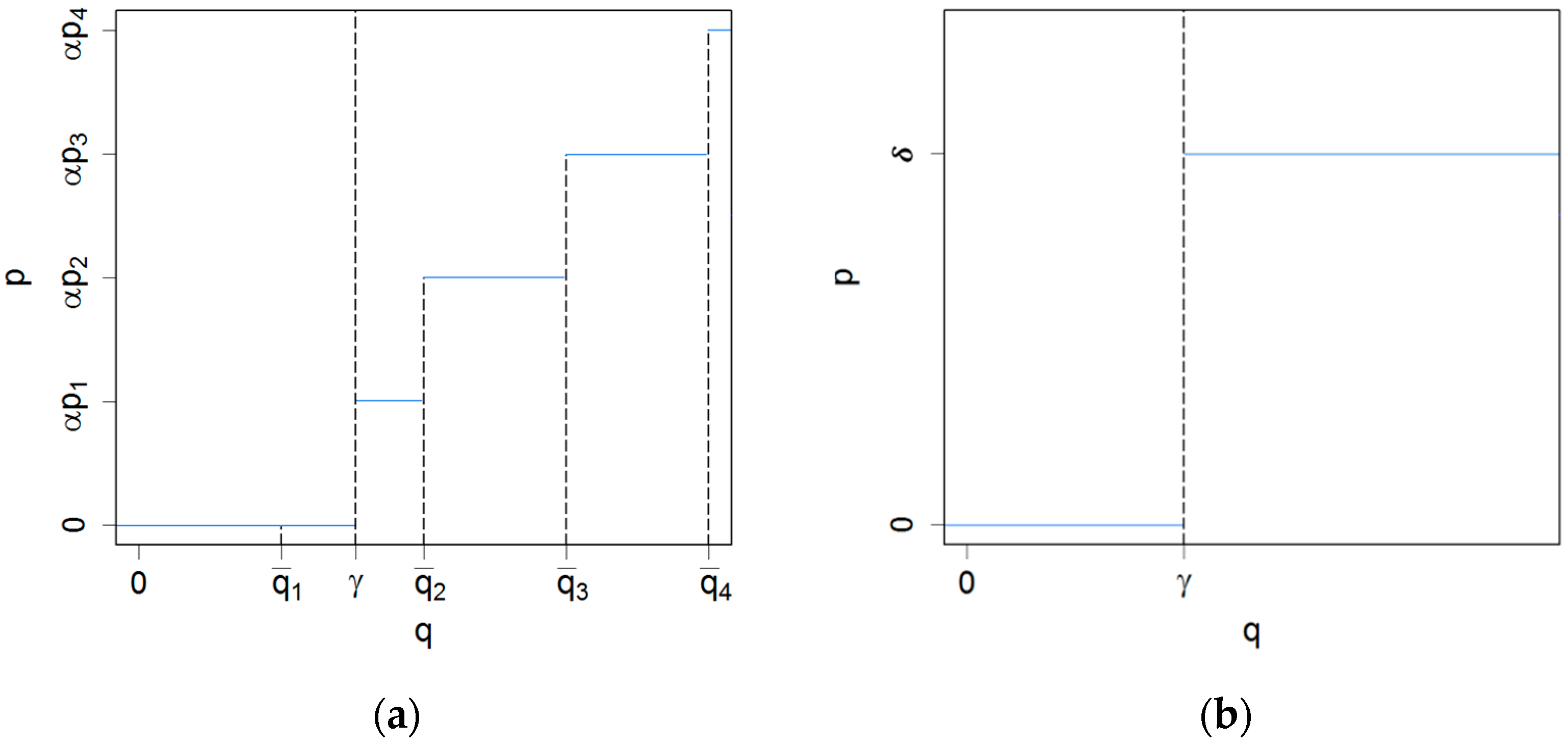
Figure 2.
Results of simulation experiment 1, analyzing modifications of the 2013 IBT: For various levels of the tariff rate multiplication factor , (a) shows the average revenue per m3 paid by all households; (b) shows the percentage of low-income households consuming less than 50 L per person per day; and (c,d) show the average revenue per m3 paid by high and low income households, respectively. The colored curves indicate the following levels of the tariff increase threshold measured in m3 per household per quarter: pink = 20; red = 30; orange = 40; yellow = 50; blue = 60; green = 70. The dotted lines indicate the baseline values reflecting the current situation. Axis labels: l/c/d = liters per capita per day; hhlds = households.

Figure 3.
Results of simulation experiment 2, analyzing a two-block tariff consisting of one block free of charge, followed by a second block with a uniform tariff rate:, where the boundary between the two blocks is defined in m3 per household per quarter: For various levels of the upper block tariff rate , (a) shows the average revenue per m3 paid by all households; (b) shows the percentage of low-income households consuming less than 50 L per person per day; and (c) and (d) show the average revenue per m3 paid by high and low income households, respectively. The colored curves indicate the following levels of the tariff increase threshold , measured in m3 per household per quarter: pink = 20; red = 30; orange = 40; yellow = 50; blue = 60; green = 70. Axis labels: l/c/d = liters per capita per day; hhlds = households.
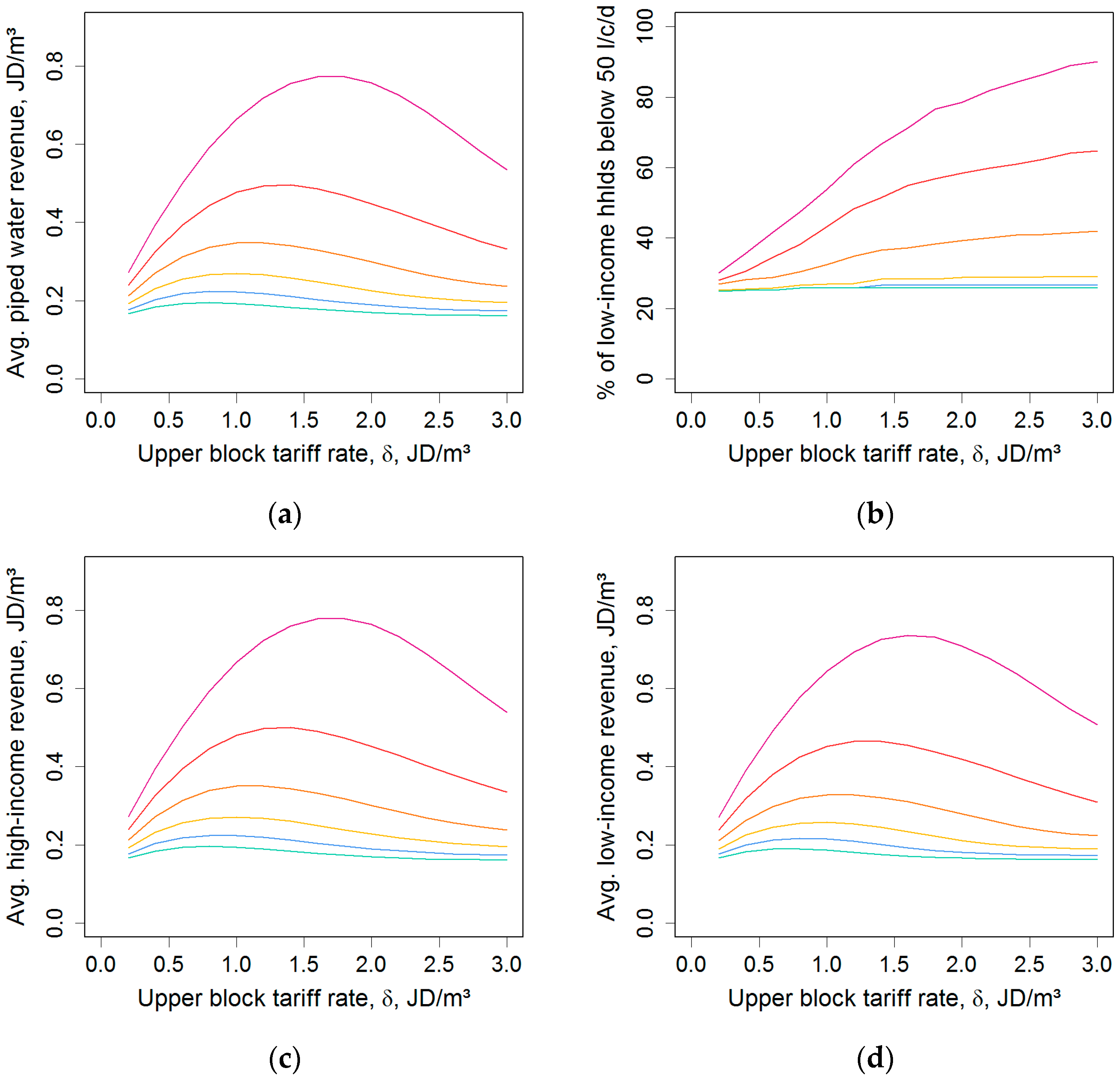
Figure 4.
Results of simulation experiment 3, analyzing a two-block tariff consisting of one block free of charge, followed by a second block with a uniform tariff rate, where the boundary between the two blocks is defined in liters per person per day: For various levels of the upper block tariff rate , (a) shows the average revenue per m3 paid by all households; (b) shows the percentage of low-income households consuming less than 50 L per person per day; and (c) and (d) show the average revenue per m3 paid by high and low income households, respectively. The colored curves indicate the following levels of the tariff increase threshold measured in liters per person per day: pink = 10; red = 20; orange = 30; yellow = 50; blue = 75; green = 100. The dotted lines mark the financial costs of water provision of 1.882 JD/m3. Axis labels: l/c/d = liters per capita per day; hhlds = households.


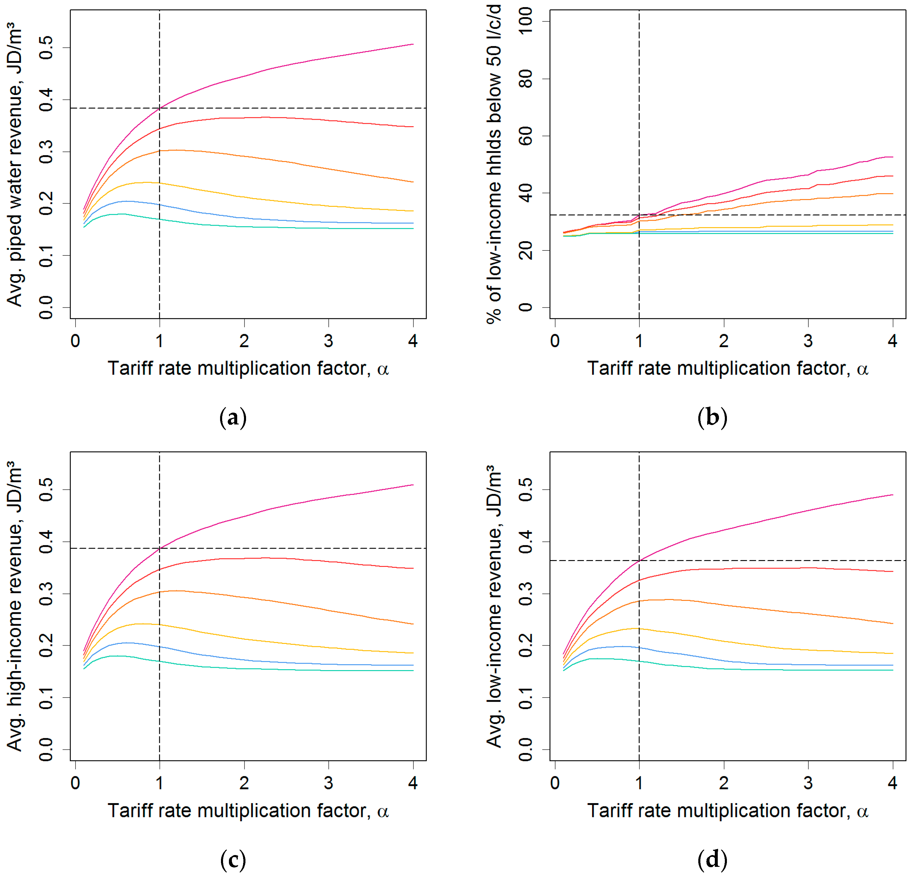
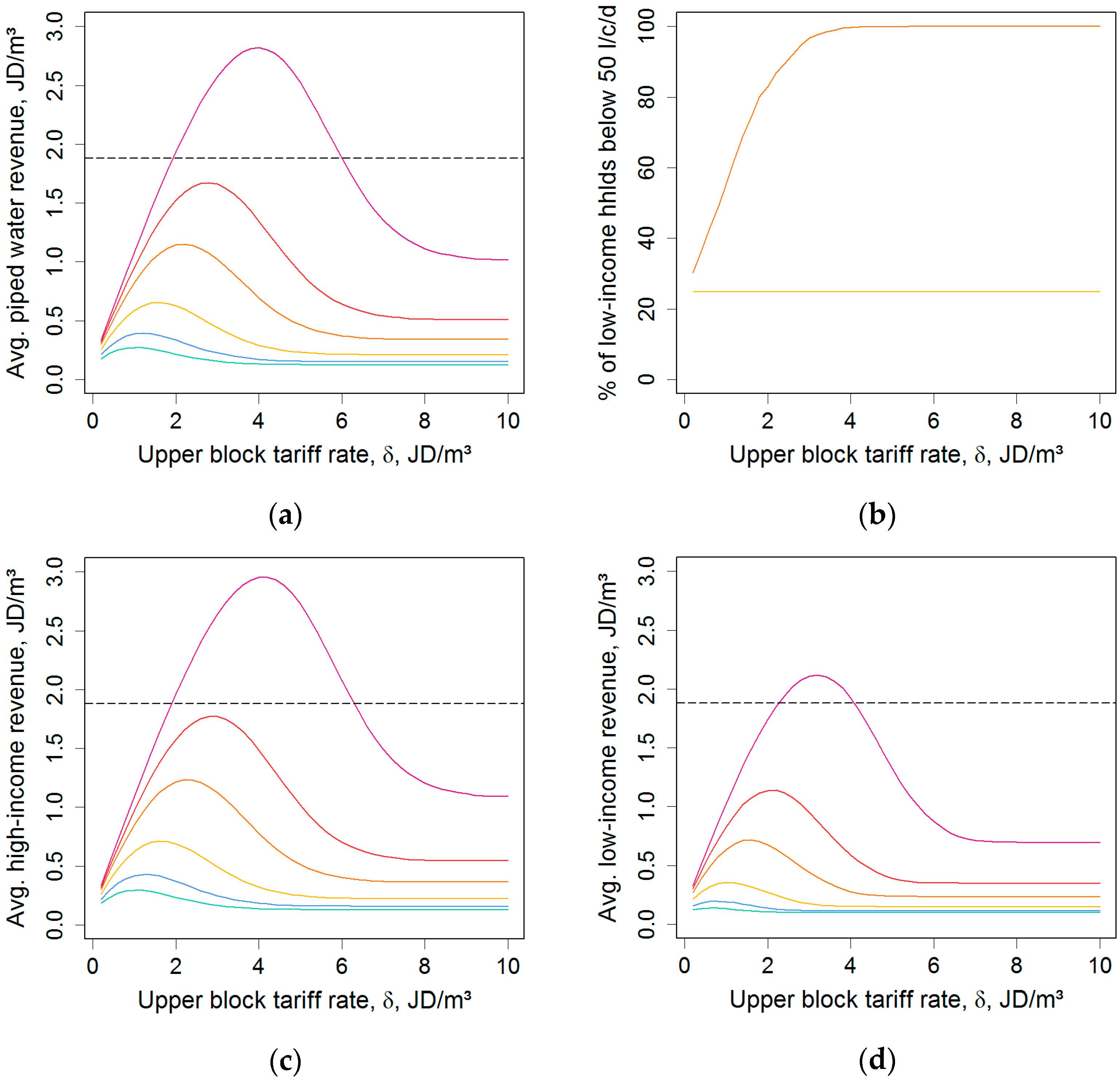
Table 1.
Descriptive statistics for relevant variables in the Jordan Household Expenditure and Income Surveys 2002, 2006, 2008, 2010, and 2013.
Table 1.
Descriptive statistics for relevant variables in the Jordan Household Expenditure and Income Surveys 2002, 2006, 2008, 2010, and 2013.
| Variable | Units | Weighted | Min. | Max. | |
|---|---|---|---|---|---|
| Mean | Std. Dev. | ||||
| Household water demand (q) | m3/qtr. | 46.7084 | 31.9897 | 18.0 | 812.7 |
| Marginal Price (p) | JD/m3 | 0.5261 | 0.5546 | 0 | 4.8 |
| Income (y) | JD/a | 9469.8 | 10,965.6 | 84.0 | 844,349.1 |
| Virtual Income (y + d) | JD/qtr. | 9537.3 | 11,003.2 | 109.2 | 845,057.2 |
| No. of Adults (ADT) | Count | 3.7107 | 1.9786 | 1 | 15 |
| No. of Children (CHD) | Count | 1.8549 | 1.7735 | 0 | 12 |
| No. of Seniors (SEN) | Count | 0.2440 | 0.5312 | 0 | 3 |
| Marital Status (MAR) | Boolean | 0.8519 | 0.3552 | 0 | 1 |
| Higher Education Spouse (EDU) | Boolean | 0.1941 | 0.3955 | 0 | 1 |
| Own Residence (OWN) | Boolean | 0.7139 | 0.4520 | 0 | 1 |
| Large Residence (LGR) | Boolean | 0.1609 | 0.3674 | 0 | 1 |
| Rural/Urban (URB) | Boolean | 0.82984 | 0.37577 | 0 | 1 |
Notes: Mean and standard deviation are weighted by observation weights from the DOS HEIS datasets. JD = Jordanian Dinar, qtr. = quarter year.
Table 2.
Estimates of the natural logarithm of quarterly household water demand under various models.
Table 2.
Estimates of the natural logarithm of quarterly household water demand under various models.
| Variable | 2013 Only | All Years | |||||
|---|---|---|---|---|---|---|---|
| OLS1 | OLS2 | DCC | OLS1 | OLS2 | DCC | ||
| Intercept | 3.2674*** (0.0522) | 2.2834*** (0.0913) | 1.9885*** (0.1508) | 3.3217*** (0.0343) | 1.9951*** (0.0590) | 1.4587*** (0.1019) | |
| 0.6065*** (0.0059) | – | −0.1877** (0.0602) | 0.7798*** (0.0043) | - | −0.4510*** (0.0601) | ||
| 0.0014 (0.0064) | 0.1216*** (0.0111) | 0.1536*** (0.0186) | −0.0067 (0.0042) | 0.1526*** (0.0071) | 0.2181*** (0.0125) | ||
| 0.0658*** (0.0085) | 0.1612*** (0.0150) | 0.2010*** (0.0162) | 0.0386*** (0.0047) | 0.1345*** (0.0081) | 0.1852*** (0.0132) | ||
| −0.0041*** (0.0009) | −0.0117*** (0.0016) | −0.0149*** (0.0016) | −0.0018*** (0.0005) | −0.0084*** (0.0008) | −0.0113*** (0.0012) | ||
| 0.0222*** (0.0024) | 0.0391*** (0.0043) | 0.0445*** (0.0054) | 0.0085*** (0.0015) | 0.0236*** (0.0026) | 0.0313*** (0.0038) | ||
| −0.0024 (0.0070) | 0.0492*** (0.0125) | 0.0612*** (0.0183) | −0.0124** (0.0045) | 0.0286*** (0.0079) | 0.0443*** (0.0116) | ||
| −0.0111 (0.0101) | −0.0372* (0.0180) | −0.0382 (0.0238) | 0.0076 (0.0068) | −0.0258* (0.0120) | −0.0423* (0.0167) | ||
| −0.0107 (0.0088) | −0.0569*** (0.0156) | −0.0638** (0.0221) | −0.0169** (0.0060) | −0.0409*** (0.0106) | −0.0542*** (0.0145) | ||
| 0.0595*** (0.0085) | 0.1337*** (0.0150) | 0.1421*** (0.0204) | 0.0762*** (0.0054) | 0.1493*** (0.0095) | 0.1673*** (0.0127) | ||
| 0.0115 (0.0108) | 0.0673*** (0.0192) | 0.1109*** (0.0300) | 0.0031 (0.0075) | 0.1055*** (0.0132) | 0.1546*** (0.0195) | ||
| −0.1993*** (0.0092) | −0.2218*** (0.0164) | −0.2430*** (0.0221) | −0.1970*** (0.0060) | −0.1951*** (0.0105) | −0.2268*** (0.0157) | ||
| N | 4847 | 4847 | 4847 | 15,811 | 15,811 | 15,811 | |
| RSE | 0.2094 | 0.3728 | - | 0.2764 | 0.4857 | - | |
| - | - | 0.0355 (0.0372) | - | - | 0.3315*** (0.0175) | ||
| - | - | 0.4167*** (0.0053) | - | - | 0.3996*** (0.0106) | ||
| R² | 0.7472 | 0.1984 | - | 0.7344 | 0.1797 | - | |
| Log-Likelihood | - | - | −2097.41 | - | - | −10,938.12 | |
Notes: * Significant at α = 0.05, ** at α = 0.01, *** at α = 0.001. Standard errors are listed in parenthesis below the coefficient estimates.
Table 3.
Estimates of the price elasticity of household water demand for different subsets of observations, based on the price coefficient from the all-year semi-log DCC.
Table 3.
Estimates of the price elasticity of household water demand for different subsets of observations, based on the price coefficient from the all-year semi-log DCC.
| Price Elasticities by Observation Subset | Price Elasticities by 2013 Tariff Block | ||
|---|---|---|---|
| All Observations (0.5261 JD/m3) | −0.2373 | Tariff Block 1 (0 JD/m3) | 0 |
| All 2013 Observations (0.5812 JD/m3) | −0.2621 | Tariff Block 2 (0.1541 JD/m3) | −0.0695 |
| 2013 Income Quintile 1 a (0.3671 JD/m3) | −0.1656 | Tariff Block 3 (0.6203 JD/m3) | −0.2798 |
| 2013 Income Quintile 2 a (0.4949 JD/m3) | −0.2232 | Tariff Block 4 (1.0665 JD/m3) | −0.4810 |
| 2013 Income Quintile 3 a (0.5473 JD/m3) | −0.2468 | Tariff Block 5 (1.3612 JD/m3) | −0.6139 |
| 2013 Income Quintile 4 a (0.6418 JD/m3) | −0.2895 | Tariff Block 6 (1.8599 JD/m3) | −0.8388 |
| 2013 Income Quintile 5 a (0.8067 JD/m3) | −0.3638 | Tariff Block 7 (3.2040 JD/m3) | −1.4450 |
Notes: Values in the left column are calculated across all observations, if not otherwise stated. All values in the right column are derived with variable inputs from the 2013 observations only. Values in parentheses indicate the average tariff rate paid for the marginal tariff block across the relevant subset of observations. a Differences in elasticity by income group result only from the differences in the marginal tariff currently paid.
Table 4.
Piped water tariff structures for residential users in Jordan, 2011–2016.
| Governorates Served by Companies | Governorates Served by WAJ | ||||||||
|---|---|---|---|---|---|---|---|---|---|
| Blocks | Variable Rate | Fixed Charge | Blocks | Variable Rate | Fixed Charge | ||||
| m3/qtr. | Water | WW | Water | WW | m3/qtr. | Water | WW | Water | WW |
| 0–20 | 0 | 0 | 4.53 | 0.6 | 0–18 | 0 | 0 | 3.9 | 0.6 |
| 20–38 | 0.145 | 0.04 | 6.18 | 0.6 | 18–36 | 0.075 | 0.04 | 5.1 | 0.6 |
| 38–56 | 0.5 | 0.25 | 7.83 | 0.6 | 36–54 | 0.4 | 0.2 | 6.75 | 0.6 |
| 56–74 | 0.935 | 0.495 | 7.83 | 0.6 | 54–72 | 0.715 | 0.33 | 6.75 | 0.6 |
| 74–92 | 1.15 | 0.69 | 7.83 | 0.6 | 72–90 | 0.748 | 0.345 | 6.75 | 0.6 |
| 92–128 | 1.61 | 0.805 | 7.83 | 0.6 | 90–126 | 1.15 | 0.575 | 6.75 | 0.6 |
| ≥128 | 3.2 | 1.6 | 7.83 | 0.6 | ≥126 | 1.44 | 0.84 | 6.75 | 0.6 |
Notes: Water = water supply tariffs, WW = wastewater tariffs, qtr. = quarter year. Each variable rate is only applied to the quantity consumed within its block. Fixed charges are not cumulative. Consumers only pay the fixed charge listed in the row of their highest consumption block.
Table 5.
Parameter values in the simulation of IBT modifications.
| Simulation Experiment | Tariff Rate Multiplication Factor | Tariff Increase Threshold Value | Upper Block Tariff Rate, in JD/m3 | |||||
|---|---|---|---|---|---|---|---|---|
| Min. | Incr. | Max. | Unit | Values | Min. | Incr. | Max. | |
| 1 | 0.1 | 0.1 | 4.0 | m3/qtr. | 20, 30, 40, 50, 60, 70 | - | - | - |
| 2 | - | - | - | m3/qtr. | 20, 30, 40, 50, 60, 70 | 0.2 | 0.2 | 3.0 |
| 3 | - | - | - | L/day | 10, 20, 30, 50, 75, 100 | 0.2 | 0.2 | 10.0 |
Notes: Min. = minimum parameter value; incr. = increment by which the parameter value is changed; max. = maximum parameter value; qtr. = quarter year. For each of the simulation experiments, one simulation run is conducted for each possible combination of the listed parameter values.
© 2018 by the authors. Licensee MDPI, Basel, Switzerland. This article is an open access article distributed under the terms and conditions of the Creative Commons Attribution (CC BY) license (http://creativecommons.org/licenses/by/4.0/).
Share and Cite
MDPI and ACS Style
Klassert, C.; Sigel, K.; Klauer, B.; Gawel, E. Increasing Block Tariffs in an Arid Developing Country: A Discrete/Continuous Choice Model of Residential Water Demand in Jordan. Water 2018, 10, 248. https://doi.org/10.3390/w10030248
AMA Style
Klassert C, Sigel K, Klauer B, Gawel E. Increasing Block Tariffs in an Arid Developing Country: A Discrete/Continuous Choice Model of Residential Water Demand in Jordan. Water. 2018; 10(3):248. https://doi.org/10.3390/w10030248
Chicago/Turabian StyleKlassert, Christian, Katja Sigel, Bernd Klauer, and Erik Gawel. 2018. "Increasing Block Tariffs in an Arid Developing Country: A Discrete/Continuous Choice Model of Residential Water Demand in Jordan" Water 10, no. 3: 248. https://doi.org/10.3390/w10030248
Note that from the first issue of 2016, this journal uses article numbers instead of page numbers. See further details here.