Identification of a Contaminant Source Location in a River System Using Random Forest Models

Abstract

We consider the problem of identifying the source location of a contaminant via analyzing changes in concentration levels observed by a sensor network in a river system. To address this problem, we propose a framework including two main steps: (i) pre-processing data; and (ii) training and testing a classification model. Specifically, we first obtain a data set presenting concentration levels of a contaminant from a simulation model, and extract numerical characteristics from the data set. Then, random forest models are generated and assessed to identify the source location of a contaminant. By using the numerical characteristics from the prior step as their inputs, the models provide outputs representing the possibility, i.e., a value between 0 and 1, of a spill event at each candidate location. The performance of the framework is tested on a part of the Altamaha river system in the state of Georgia, United States of America.

1. Introduction

Many scholars and practitioners have explored technologies for monitoring water quality because of urbanization, industrialization, climate change, and threats related to terrorism. Among these technologies, identifying the source location of a contaminant in groundwater and river systems has been significantly improved by the development of sensors and data analytics. Rapid identification of contaminant source location enables us to reduce the risk of contaminant exposure by preventing pollution events and providing fast responses to undesired phenomena caused by such events.

Most past research works on identifying contaminant source locations have focused on groundwater systems. Gorelick et al. [1], Aral and Guan [2], Aral et al. [3], Sun et al. [4], and Singh and Datta [5] adopted optimization algorithms, such as linear and non-linear programming algorithms as well as meta-heuristic algorithms, to identify the source location of a contaminant in groundwater systems. Instead of optimization algorithms, some statistical methods, such as a backward probability model approach [6,7] and a geostatistical approach [8], were used for similar problems. In addition, Singh et al. [9], Singh and Datta [10] and Srivastava and Singh [11] employed an artificial neural network model to efficiently identify the source location of a contaminant in a groundwater system.

For river systems, there are relatively few studies regarding the identification of a contaminant source because of the size of such systems and the complexity of the corresponding problems. Boano et al. [12] used a geostatistical approach to generate historical information related to a pollutant when the source location is known. Chen et al. [13] employed multivariate statistical methods to determine spatial and temporal variations in water quality and to identify the contaminant source in a lake. Ghane et al. [14] applied the backward probability method to identify the source location and the release time of pollutants in a river system. In this paper, we focused on a river system and sought to identify the source location of a contaminant spill.

The research of Telci and Aral [15] is most closely related to ours. This work considers the problem of identifying the source location of a single instantaneous contaminant among given candidate locations in a river system while considering uncertainties in spill and rainfall events. They used estimates of statistical changes in concentration levels over time, as shown in Grubner [16]. Then, they applied an adaptive sequential feature selection algorithm developed by Jiang [17] to sequentially screen possible candidate locations of the contaminant source in a river system. Although their sensor network includes more than one sensor, Telci and Aral [15] do not consider relative information among sensors as an input. Moreover, the final result of the adaptive sequential feature selection algorithm is only a single source location index, and thus one cannot evaluate how reliable the identified location is. In this paper, we suggest a way to preprocess data related to changes in contamination levels and use relative information observed by pairs of sensors. We construct random forest models and provide a measure of the possibility that each candidate location is identical to the correct location of the contaminant source, reported as a number between 0 and 1. As a result, a decision maker can quantitatively evaluate the possibility of the results from the model.

This paper is organized as follows. Section 2 provides notations and the problem description. In Section 3, we provide a two-step framework to effectively identify the source location of a contaminant including data pre-processing and model generation and assessment. Section 4 presents experimental results of a case study, and concluding remarks follow in Section 5.

2. Background

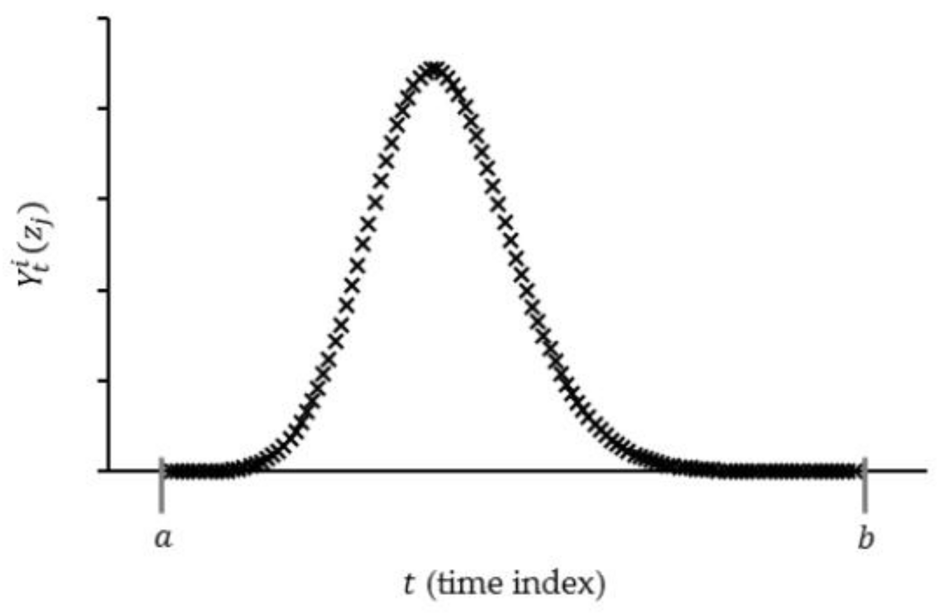
2.1. Problem Description

In the river system, there are $N$ candidate locations at which a monitoring sensor can be installed or where a spill event may occur. Let $D$ be the index set of the candidate locations, $D=\left\{1,2,\dots ,N\right\}$ and $K$ be the number of sensors in the river system such that $2\le K\le N$ because we consider a network system with multiple sensors. A vector $z$ represents location indices of $K$ sensors, $z=\left(z_1,\dots ,z_K\right)$, such that $z_j\in D$, for $j=1,\dots ,K$ and we assume $z_1<z_2<\dots <z_K$ to avoid repetition. In this paper, we consider the case where $K$ and $z=\left(z_1,\dots ,z_K\right)$ are given.

Each sensor returns a concentration level of the contaminant at time index $t$ for $t=1,..,T.$ Let $Y_t\left(z_j\right)$ denote the concentration level at time index $t$ that is monitored by the sensor located at $z_j$ for $t=1,..,T$ and $j=1,..,K$. Then, a collection of the concentration levels monitored by $K$ sensors over all time indices is denoted by:

$$\mathit{Y}\left(z\right)=\left[\begin{array}{ccc}{Y}_1\left(z_1\right)& \dots & Y_T\left(z_1\right)\\ ⋮& \ddots & ⋮\\ Y_1\left(z_K\right)& \dots & Y_T\left(z_K\right)\end{array}\right]$$

(1)

For all $d\in D$, we denote $P\left(d\right)$ as a measure representing the possibility that location $d$ is identical to the correct spill location. Note that $0\le P\left(d\right)\le 1$ for all $d\in D$. The closer $P\left(d\right)$ is to 1, the more likely it is that a spill event has occurred at location index $d$. Let $\mathit{P}$ denote a vector of $P\left(d\right)$ as follows:

$$\mathit{P}=\left[\begin{array}{c}P\left(1\right)\\ ⋮\\ P\left(N\right)\end{array}\right]$$

(2)

The main purpose of the paper is to construct a data-driven model which evaluates $\mathit{P}$ for a given $\mathit{Y}\left(z\right)$ as shown in Figure 1. To construct the data-driven model, we first need to prepare large-sized training data that can be obtained from a hydrodynamics simulation. In the next section, we briefly describe the hydrodynamics simulation considering random contaminant spill and rainfall events.

2.2. Hydrodynamics Simulation

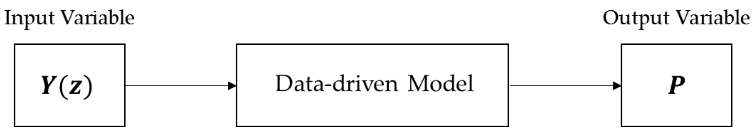
A simulation software package was employed to get observations of $\mathit{Y}\left(z\right)$ and $\mathit{P}$. The Storm Water Management Model (SWMM) is a popular software package for simulating the hydrodynamics and contaminant transportation in a river system. The SWMM was developed and released by the Environmental Protection Agency (EPA) of the United States of America, and it was designed for simulating hydrodynamic systems around urban areas under dynamic flow, including rainfall events and various watershed conditions as described in Rossman [18]. To construct a simulation model within the SWMM, we need (i) fixed information representing geological and geometrical properties of the system and fundamental hydrodynamics in the system; and (ii) variable information representing random spill and rainfall events based on historical data.

For each SWMM run, fixed information is modeled as a set of constants, and variable information is modeled as a set of random variables. Note that a single instantaneous spill is considered for a spill event. The random variables describe spill and rainfall events. To describe the spill event, we denote random variables $Q^i$ and $M^i$ as the spill starting time and spill intensity of the $i$th simulation, respectively. In the case of rainfall events, we employed the method described in Telci et al. [19]. We partitioned the entire area of the river system into $\omega$ number of regions, which are called sub-catchments. Each sub-catchment has a number of pre-generated rain patterns based on historical data. Then, a rain pattern of each sub-catchment is randomly selected among the pre-generated patterns. An $\omega$—dimensional vector ${\mathit{I}}^i$ denotes an instance of rain patterns over the entire river network in the $i$th simulation run.

For the $i$th simulation, a set of random variables $(Q^i,M^i,{\mathit{I}}^i$) was generated and combined with fixed information in an input file. After executing the SWMM software with the input file, we obtained a large output file that includes concentration levels as well as various quantities regarding hydrodynamics at each candidate location at every inter-reporting time of the simulation clock. We denote ${\mathit{Y}}^i\left(z\right)$ and ${\mathit{P}}^i$ as the $i$th simulation observation of $\mathit{Y}\left(z\right)$ and $\mathit{P}$. Similarly, $Y_t^i\left(z_j\right)$ and $P^i\left(d\right)$ represent the $i$th simulation observation of $Y_t\left(z_j\right)$ and $P\left(d\right)$. Therefore,

$${\mathit{Y}}^i\left(z\right)=\left[\begin{array}{ccc}{Y}_1^i\left(z_1\right)& \dots & Y_T^i\left(z_1\right)\\ ⋮& \ddots & ⋮\\ Y_1^i\left(z_K\right)& \dots & Y_T^i\left(z_K\right)\end{array}\right]\text{ and }{\mathit{P}}^i=\left[\begin{array}{c}{P}^i\left(1\right)\\ ⋮\\ P^i\left(N\right)\end{array}\right].$$

(3)

We obtained values of ${\mathit{Y}}^i\left(z\right)$ from the large output and constructed ${\mathit{P}}^i$ by assigning 1 for the correct spill location and 0 elsewhere.

3. Method

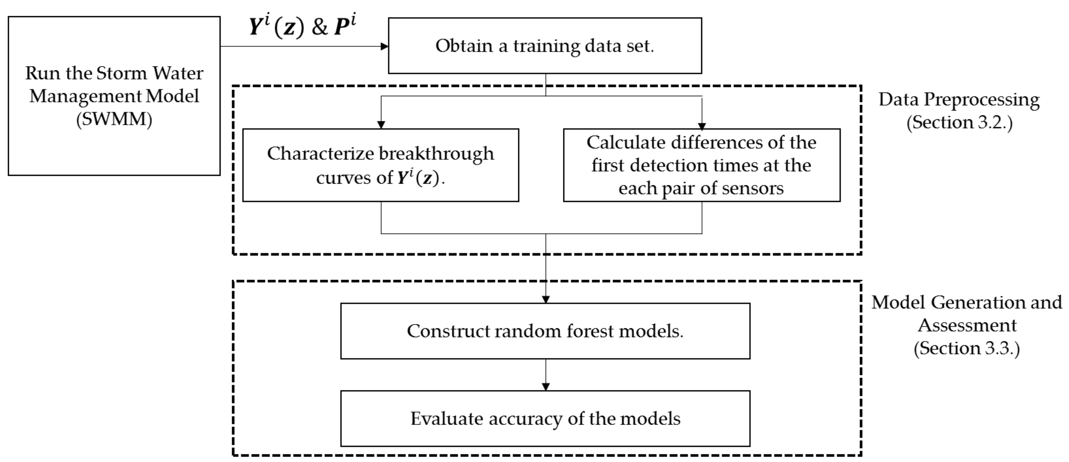
3.1. Overall Workflow

In this section, we suggest a framework to identify the source location of a contaminant spill through a classification model with simulation data. The overall workflow of the proposed framework is presented in Figure 2. The framework consists of two main steps, including pre-processing simulation data and generating and evaluating a classification model. As described in Section 2.2, a SWMM run with an input file returns ${\mathit{Y}}^i\left(z\right)$ and ${\mathit{P}}^i$. We quantitatively characterize changes of non-zero concentration levels whose shape is called the breakthrough curve, and we calculated relative time indices observed by each pair of sensors (see Section 3.2). After pre-processing ${\mathit{Y}}^i\left(z\right)$, we constructed and evaluated a classification model (see Section 3.3).

3.2. Data Pre-Processing

Using ${\mathit{Y}}^i\left(z\right)$ to directly construct a data-driven model causes two main issues. First, the size of ${\mathit{Y}}^i\left(z\right)$ is $K\times T$, and it becomes extremely large as the number of discretized time indices increases. Note that $T$ is often a couple of thousand in practice, and thus it is problematic. Second, when we keep track of $Y_1^i\left(z_j\right), \dots , Y_T^i\left(z_j\right)$ for a fixed $z_j$, most of the values are reported as zeros, and non-zero values consecutively appear under a single, instantaneous spill. Therefore, we need to handle $Y_1^i\left(z_j\right), \dots , Y_T^i\left(z_j\right)$ for a fixed $z_j$ efficiently.

We focused on characterizing non-zero values of $Y_t^i\left(z_j\right)$ if any contaminant mass is observed at $z_j$. Let $a$ and $b$ represent the time indices at which the sensor starts and ends the detection of non-zero concentration levels for the contaminant, respectively. They are expressed in the following equations:

$$a=\min \left\{t;Y_t^i\left(z_j\right)>0,t=1,\dots ,T\right\},$$

(4)

$$b=\min \left\{t;Y_t^i\left(z_j\right)>0\&Y_{t+1}^i\left(z_j\right)=0,t=1,\dots ,T\right\}.$$

(5)

Figure 3 shows a scatter plot of samples of $Y_t^i\left(z_j\right)$ for $t=a,\dots ,b$, and the plot has a curved and unimodal shape. Note that the curve is referred to as a breakthrough curve [11,15]. The breakthrough curve can be interpreted as a constant multiple of a probability density function, and thus it is characterized by using definitions of a series of statistical moments for the probability density function [15,16].

As described in Telci and Aral [15], we first estimate the central statistical moment, standard deviation, skewness, and kurtosis of the breakthrough curve by approximation using the trapezoid rule. Let $r_t$ be the time in simulation clock corresponding to time index $t$. For $Y_t^i\left(z_j\right)$, $t=a,\dots ,b$, the estimated first moment is denoted by $\overline{{\mu }_1^i\left(z_j\right)}$, and it is calculated by:

$$\overline{{\mu }_1^i\left(z_j\right)}=\frac{{{\displaystyle \sum }}_{t=a}^{b-1}\left[Y_t^i\left(z_j\right)r_t+Y_{t+1}^i\left(z_j\right)r_{t+1}\right]\left(r_{t+1}-r_t\right)}{{{\displaystyle \sum }}_{t=a}^{b-1}\left[Y_t^i\left(z_j\right)+Y_{t+1}^i\left(z_j\right)\right]\left(r_{t+1}-r_t\right)}.$$

(6)

For $Y_t^i\left(z_j\right)$, $t=a,\dots ,b$, the estimated $k$th central moment, for $k=2, 3, \dots$, is denoted by $\overline{m_k^i\left(z_j\right)}$ and it is calculated by:

$$\overline{m_k^i\left(z_j\right)}=\frac{{{\displaystyle \sum }}_{t=a}^{b-1}\left[Y_t^i\left(z_j\right){\left(r_t-\overline{{\mu }_1^i\left(z_j\right)}\right)}^k+Y_{t+1}^i\left(z_j\right){\left(r_t-\overline{{\mu }_1^i\left(z_j\right)}\right)}^k\right]\left(r_{t+1}-r_t\right)}{{{\displaystyle \sum }}_{t=a}^{b-1}\left[Y_t^i\left(z_j\right)+Y_{t+1}^i\left(z_j\right)\right]\left(r_{t+1}-r_t\right)}.$$

(7)

Let ${\sigma }^i\left(z_j\right)$, $S^i\left(z_j\right)$, and $E^i\left(z_j\right)$ be the estimated standard deviation, skewness and kurtosis of the breakthrough curve corresponding to $Y_t^i\left(z_j\right)$, $t=a,\dots ,b$. Using Equations (6) and (7), ${\sigma }^i\left(z_j\right)$, $S^i\left(z_j\right)$, and $E^i\left(z_j\right)$ are calculated as follows:

$${\sigma }^i\left(z_j\right)=\sqrt{\overline{m_2^i\left(z_j\right)}},$$

(8)

$$S^i\left(z_j\right)=\frac{\overline{m_3^i\left(z_j\right)}}{{\left({\sigma }^i\left(z_j\right)\right)}^3},$$

(9)

$$E^i\left(z_j\right)=\frac{\overline{m_4^i\left(z_j\right)}}{{\left({\sigma }^i\left(z_j\right)\right)}^4}-3.$$

(10)

If there is no positive $Y_t^i\left(z_j\right)$ for all $t=1,\dots ,T$, one may assign ${\sigma }^i\left(z_j\right)=C$, $S^i\left(z_j\right)=-C,$ and ${}^i\left(z_j\right)=-C$, where $C$ is a large positive constant.

In addition to ${\sigma }^i\left(z_j\right)$, $S^i\left(z_j\right)$, and $E^i\left(z_j\right)$, we introduce two more quantitative characteristics $U^i\left(z_j\right)$ and $A^i\left(z_j\right)$, which represent estimates of the total area and the time-averaged area between the horizon axis and the breakthrough curve, respectively, as described in Srivastava and Singh [11]. Using the left Riemann sum, they can be calculated by:

$$U^i\left(z_j\right)={{\displaystyle \sum }}_{t=a}^{b-1}{Y}_t^i\left(z_j\right)\left(r_{t+1}-r_t\right),$$

(11)

$$A^i\left(z_j\right)=\frac{{{\displaystyle \sum }}_{t=a}^{b-1}{Y}_t^i\left(z_j\right)\left(r_{t+1}-r_t\right)}{\left(r_b-r_a\right)}.$$

(12)

Using Equations (8)–(12), a series of data sets $Y_1^i\left(z_j\right), \dots , Y_T^i\left(z_j\right)$ for a fixed $z_j$ can be transformed into a 5-dimensional vector as follows:

$${\mathit{B}}^i\left(z_j\right)=\left[{\sigma }^i\left(z_j\right),S^i\left(z_j\right),E^i\left(z_j\right),U^i\left(z_j\right),A^i\left(z_j\right)\right].$$

(13)

Therefore, when considering $K$ sensors whose locations are specified by vector $\mathit{z}$, ${\mathit{Y}}^i\left(\mathit{z}\right)$ can be transformed into the $5K$ dimensional vector ${\mathit{B}}^i\left(\mathit{z}\right)$ as follows:

$${\mathit{B}}^i\left(\mathit{z}\right)=\left[{\mathit{B}}^i\left(z_1\right),\dots ,{\mathit{B}}^i\left(z_K\right)\right].$$

(14)

Since the sensor network includes at least two sensors, we may utilize relative information over different sensors regarding when non-zero $Y_t^i\left(z_j\right)$ is first detected at each sensor. Let $R^i\left(z_j\right)$ denote the time index for first detected non-zero $Y_t^i\left(z_j\right)$ such that:

$$R^i\left(z_j\right)=\{\begin{array}{ll}T,& \hfill \mathrm{if} \mathrm{the} \mathrm{sensor} \mathrm{does} \mathrm{not} \mathrm{detect} \text{a} \mathrm{contaminant};\\ \min \left\{ t |Y_t^i\left(z_j\right)>0,t=1,\dots ,T\right\},& \hfill \mathrm{otherwise}.\end{array}$$

(15)

Then, we define $R^i\left(z_p,z_q\right)$ as the difference between the times with non-zero concentration levels first detected by sensors located at $z_p$ and $z_q$, calculated by:

$$R^i\left(z_p,z_q\right)=\{\begin{array}{cc}0& ,\mathrm{if}{R}^i\left(z_p\right)=R^i\left(z_q\right);\\ R^i\left(z_p\right)-R^i\left(z_q\right)& ,\mathrm{if}{R}^i\left(z_p\right)>R^i\left(z_q\right) \mathrm{and}{R}^i\left(z_q\right)\ne T;\\ R^i\left(z_p\right)-R^i\left(z_q\right)& ,\mathrm{if}{R}^i\left(z_p\right)<R^i\left(z_q\right)\mathrm{and}{R}^i\left(z_q\right)=T;\\ R^i\left(z_q\right)-R^i\left(z_p\right)& ,\mathrm{if}{R}^i\left(z_p\right)<R^i\left(z_q\right)\mathrm{and}{R}^i\left(z_p\right)\ne T;\\ R^i\left(z_q\right)-R^i\left(z_p\right)& ,\mathrm{if}{R}^i\left(z_p\right)>R^i\left(z_q\right)\mathrm{and}{R}^i\left(z_p\right)=T.\end{array}$$

(16)

To exclude meaningless values of $R^i\left(z_p,z_q\right)$ that are due to the structure of the river system, we only considered pairs of sensors satisfying the following conditions: (i) one of the sensors should be located upstream of the other sensor; and (ii) there is no other sensor between a pair of sensors located at $z_p\mathrm{and}{z}_q$. We denote ${\mathit{R}}^i\left(\mathit{z}\right)$ as the collection of $R^i\left(z_p,z_q\right)$ for all possible pairs satisfying the above two conditions. After the pre-processing, $\left[{\mathit{B}}^i\left(\mathit{z}\right), {\mathit{R}}^i\left(\mathit{z}\right)\right]$ becomes an input vector of the classification model described in the next section.

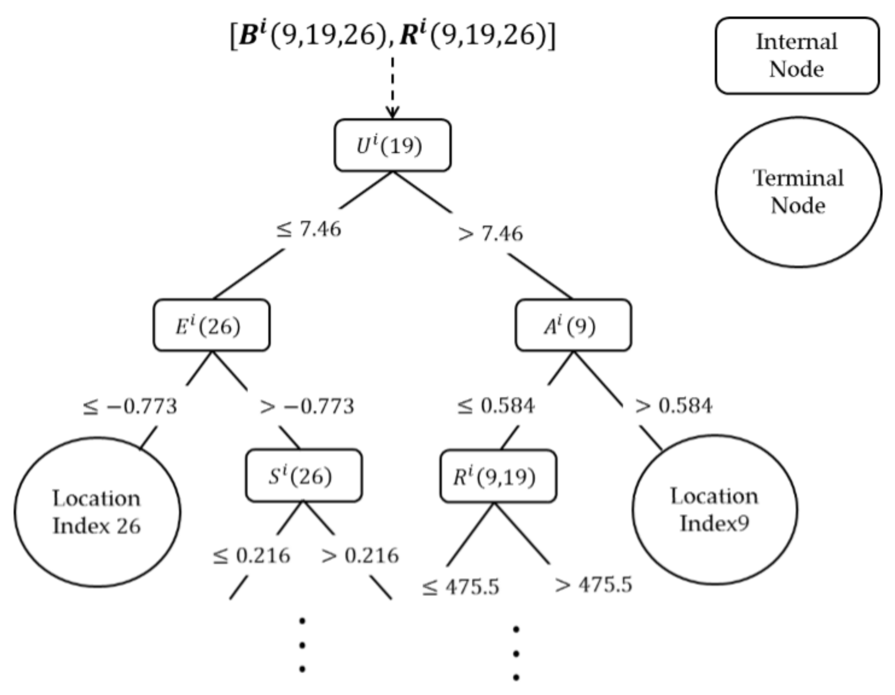
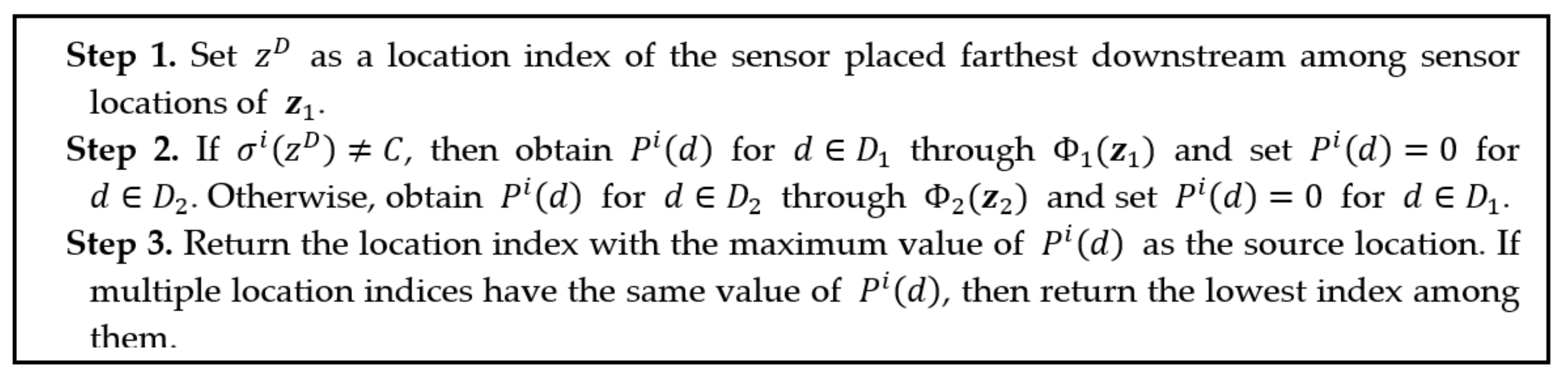
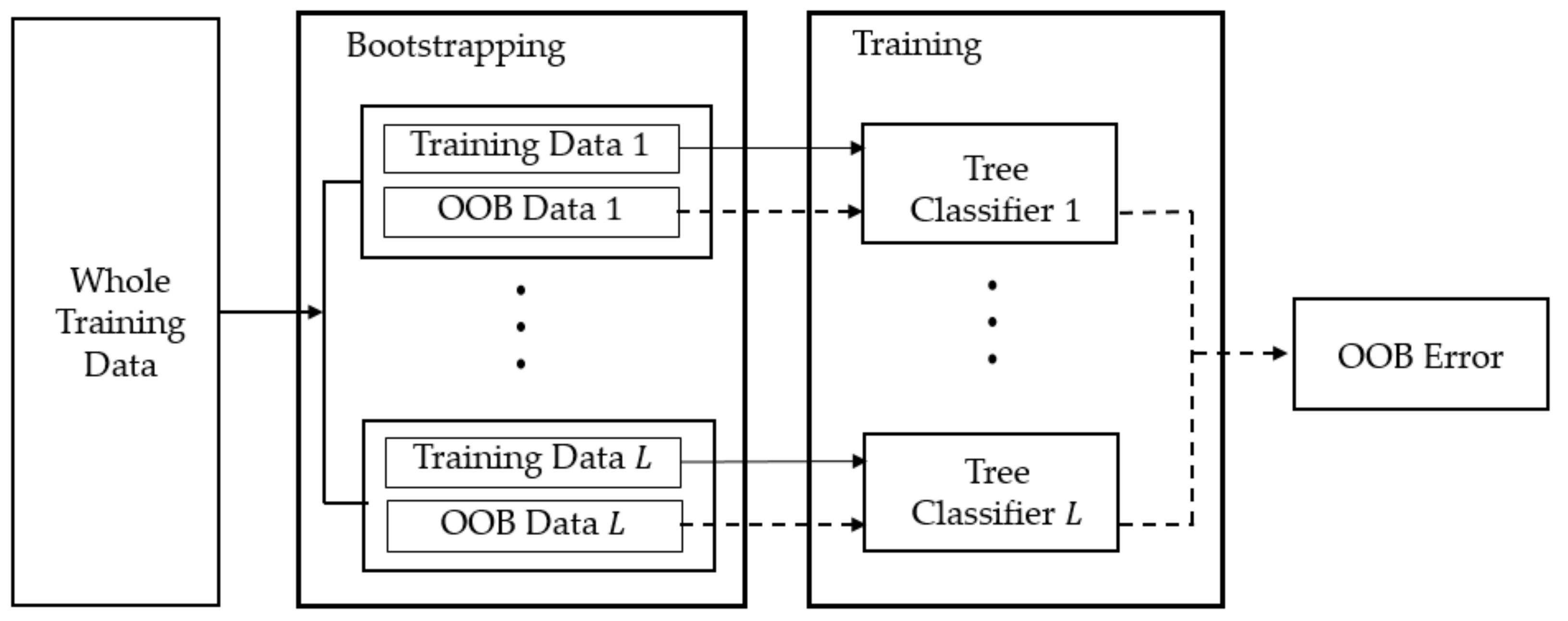
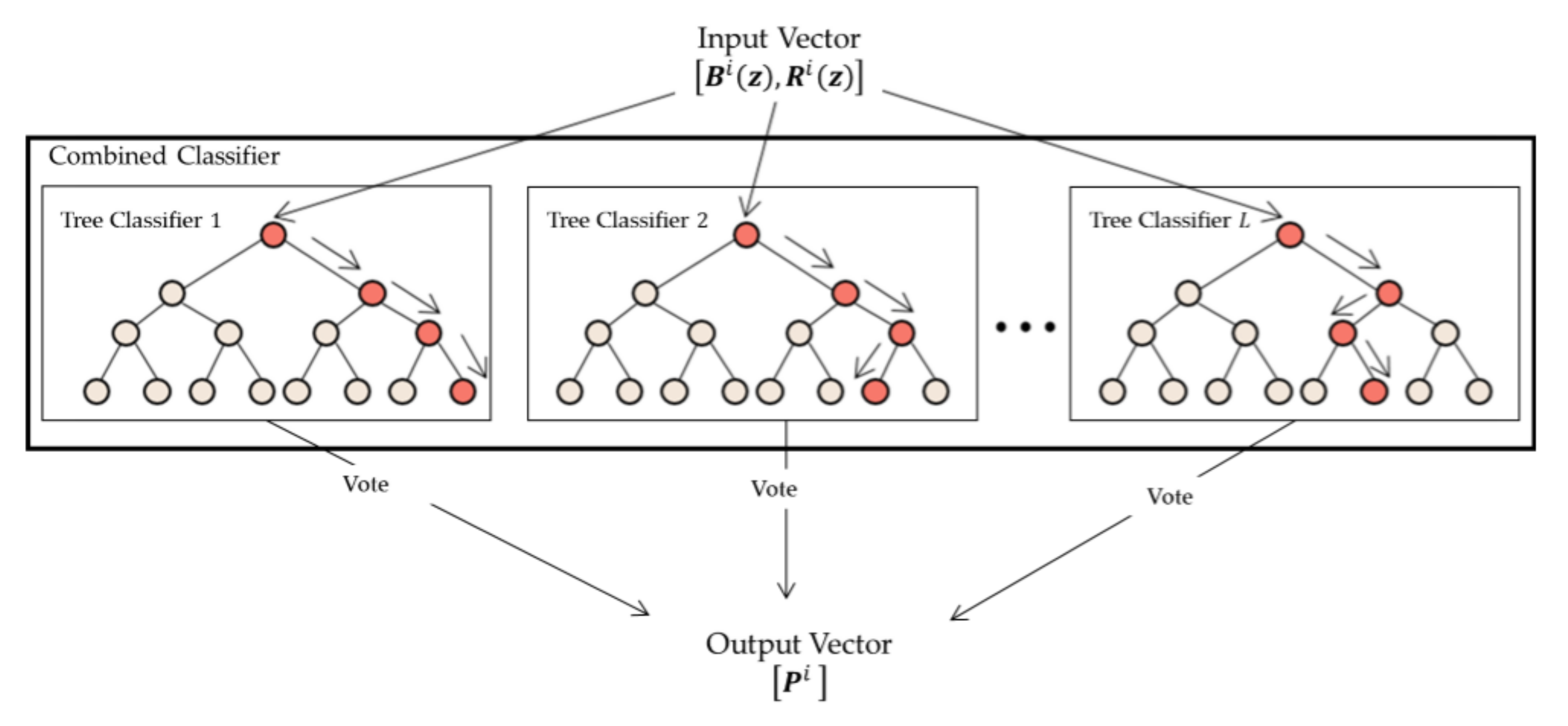
3.3. Model Generation and Assessment

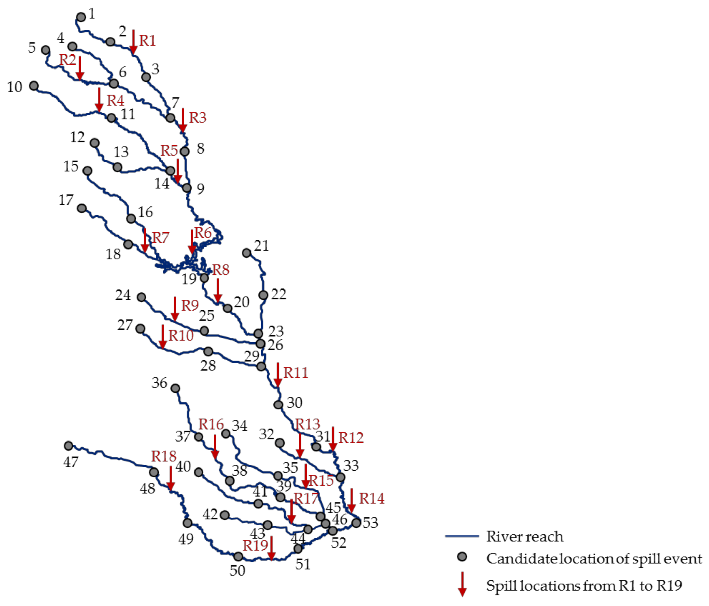
A random forest model is a popular classification model that contains a collection of tree-structured classifiers. As mentioned in Breiman [20], the random forest model has several advantages regarding accuracy, robustness and computational efficiency, compared with other classification models. Figure 4 shows the schematic flow diagram of the generation of a random forest model.

The first step of model generation is referred to as bootstrapping. In this step, the bootstrapping algorithm generates $L$ number of sample data sets from all the training data. Each sample data set exactly corresponds to a tree classifier. Approximately 2/3 of a sample data set is used as the training data to construct a tree classifier, and the remaining 1/3 of the sample data set is used as out-of-bag (OOB) data to evaluate the generalized error of the random forest model [21]. An estimate of the generalized error is called the OOB error, which is calculated by the ratio of the number of misclassified OOB data to the total number of OOB data.

In the second step of the model generation, we constructed tree classifiers represented by nodes and edges, and we trained them. In a tree classifier, there are two types of nodes, an internal node and a terminal node. At each internal node, $F$ number of input variables are randomly selected and linearly combined with their coefficients. We checked whether a linear combination of the input variables is greater than a certain constant threshold or not, and then moved to the next node. Constant thresholds and coefficients of the linear combination at each internal node can be determined by a randomized node-optimization algorithm developed by Ho [22]. This process is called training. Each terminal node corresponds to a certain final class (e.g., location index), and no further decisions or movements can occur at the terminal node.

After training, we get a combined classifier including $L$ number of tree classifiers. Note that different tree classifiers have different structures (e.g., number of nodes and arcs) and different decision rules at each internal node of the classifiers. When a vector of input values (e.g., $\left[{\mathit{B}}^i\left(\mathit{z}\right),{\mathit{R}}^i\left(\mathit{z}\right)\right]$) is entered into the model, each tree classifier selects one of the classes (e.g., location index) as a result. Figure 5 shows an example of a trained tree classifier for $z=\left(9,19,26\right)$ and $F=1$. A vector of input values, $\left[{\mathit{B}}^i\left(9,19,26\right),{\mathit{R}}^i\left(9,19,26\right)\right],$ is first entered into the node on the top of the tree, and then it moves along the edges. If $U^i\left(19\right)\le 7.46$ and $E^i\left(26\right)\le -0.773$, then the example tree concludes that location index 26 is the spill location. Each tree classifier votes for one of the classes (e.g., the location index from 1 to $N$) based on its conclusion, and the proportions of the number of votes out of the total number of tree classifiers are returned as output values (e.g., $P^i\left(d\right)$ for all $d\in D$) as shown in Figure 6.

Recall that $L$ represents the number of tree classifiers, and $F$ represents the number of input variables or input features randomly selected at each node. Selecting two parameters, $L$ and $F$, may affect the performance of the combined classifier. As $L$ increases, the generalization error gradually decreases and converges to a number. In this paper, we selected an $L$ that makes OOB errors converge. A small value of $F$ may reduce the accuracy of individual tree classifiers, but it may also reduce correlation among the trees, which decreases the generalization error. When $M$ is the number of values in an input vector, $F$ is typically selected as $\sqrt{M}$ [23,24] or $lo{g}_{2}M+1$ [20,23]. We used the $F$ selection strategy described in Breiman [25]. Based on this strategy, we checked OOB errors with $F$ values, which are all possible integers between $0.5\sqrt{M}$ and $2\sqrt{M}$ as well as between $0.5\left(lo{g}_{2}M+1\right)$ and $2\left(lo{g}_{2}M+1\right)$. Then, we selected the $F$ value with the lowest OOB error. In addition, we noted that a random forest model performs well when the number of classes is 32 or fewer [25], and thus we constructed a unified model with multiple random forest models based on partitioned classes. One way to achieve this for our problem is described in Section 4.2.

4. Case Study

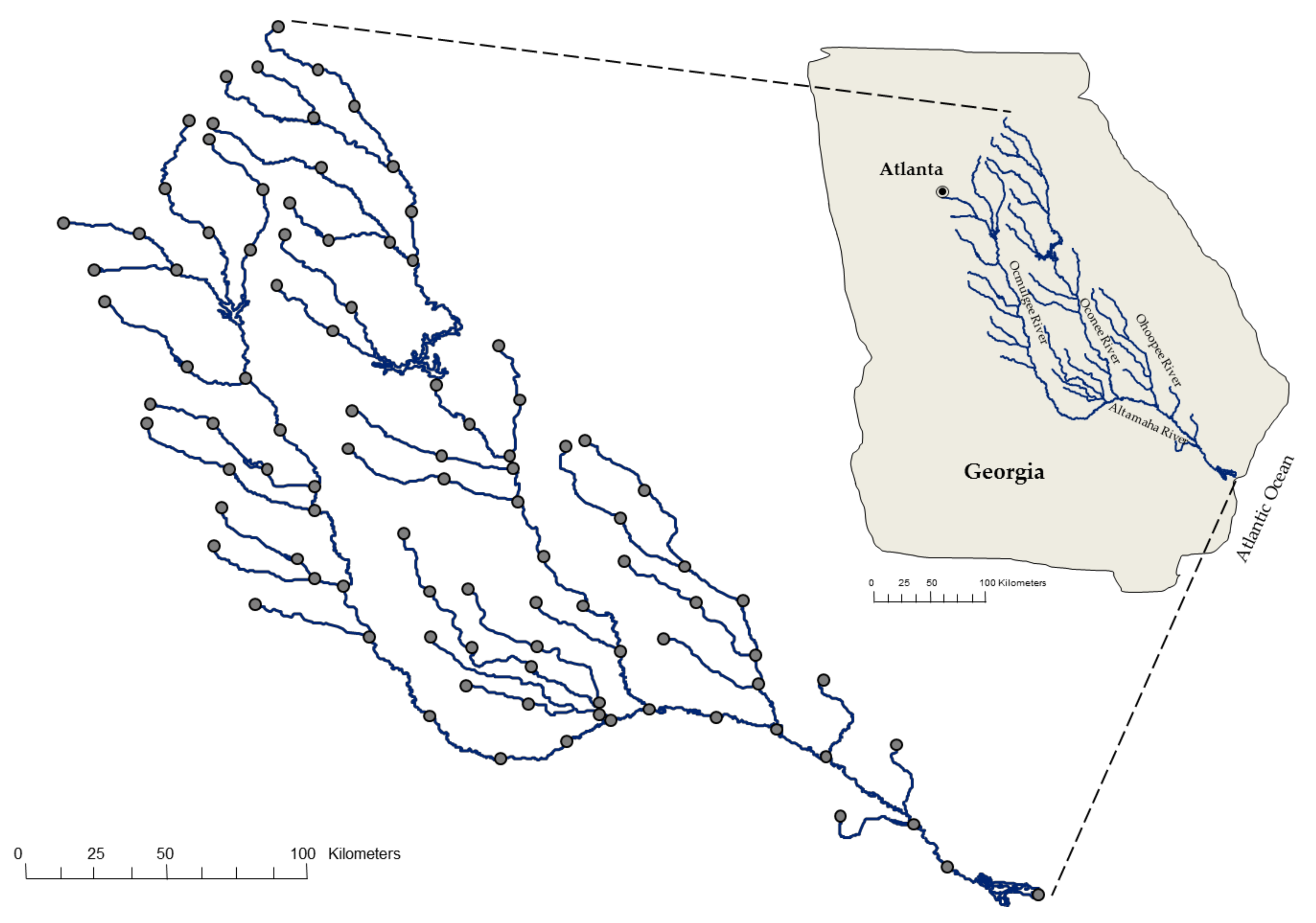
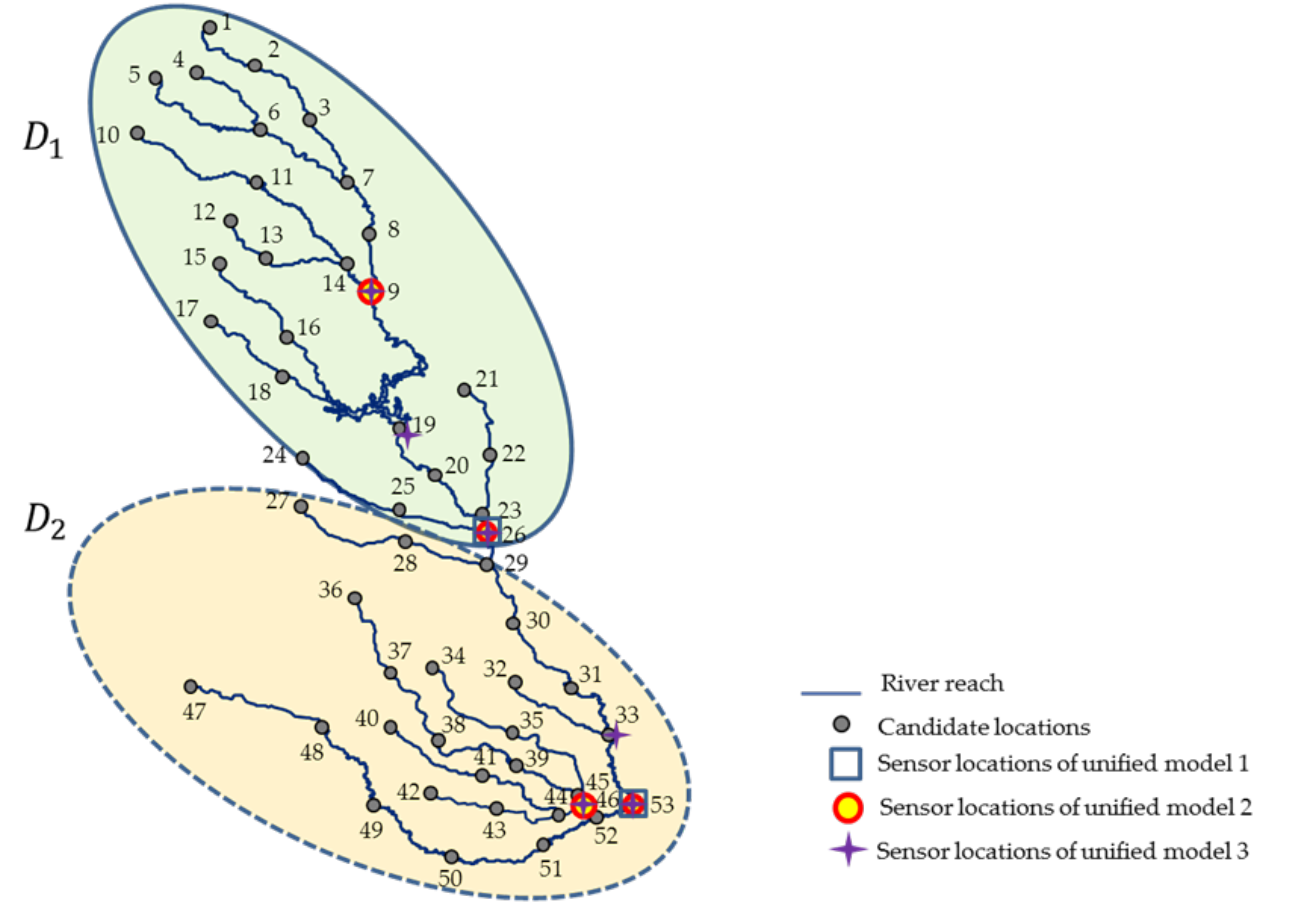
4.1. Study Area and Simulation Setup

In this section, we briefly review the study area, the Altamaha river system, and explain the method used to generate a SWMM input file for the river system. The Altamaha river system has the largest watershed in the state of Georgia, United Sates of America (31°57′33″ N; 82°32′37″ W), and it flows south-eastward to the Atlantic Ocean. The length and size of the river system are approximately 760 km (470 miles) and 36,260 km² (14,000 square miles). The system consists of the Ocmulgee river, the Oconee river, the Ohoopee river, and their confluence, and it includes 60 river reaches and 62 junctions, as shown in Figure 7. We selected 100 candidate locations (marked by small circles in Figure 7) which include the most upstream locations, locations of confluences, and locations evenly spaced along with each river reach. The details regarding the selection of candidate locations in the Altamaha river system are shown in Telci et al. [19].

Fixed information for the SWMM input file, which includes geological, geometrical, and fundamental hydrodynamics data of the river system, was obtained from the United States Geological Survey (USGS) in the National Elevation Dataset. The fundamental hydrodynamics of the river system included a steady-state hydraulic system, which was calibrated by data obtained from annual average flow rates measured in 2006 at twenty USGS gauging stations. Note that all lakes and impoundments were approximated as river reaches to simplify the network. Detailed information related to the river system and the corresponding fixed information used to construct the corresponding SWMM model is provided in Telci et al. [19].

We used two random events, spill and rainfall events, as variable information in the SWMM input file. For a spill event, the spill starting time and spill intensity, $Q^i$ and $M^i$, respectively, were assumed to be uniformly distributed between their lower and upper limits. The lower and upper limits of $Q^i$ are set to 0 and 10 days, respectively, and the lower and upper limits of $M^i$ were set to 10 and 1000 grams per liter. For rainfall events, the whole region of the river system was partitioned into 10 sub-catchments (i.e., $\omega =10$). The rain pattern of each sub-catchment was randomly selected among five pre-generated rain patterns. Note that each pre-generated rain pattern represented time-dependent rain events causing dynamic changes of hydrological conditions of the sub-catchment. Detailed information related to generating random variables to run a SWMM model is provided in Park et al. [26].

An input file of a SWMM run for the Altamaha river system is structured by combining fixed information and variable information, and then the SWMM is executed with the input file. Each SWMM run simulates changes in hydrodynamics and contamination levels during the 40 days and reports related quantitative values (e.g., concentration levels, flow rates, and the amounts of overflows) at each candidate location every 15 min in the simulation clock.

4.2. Random Forest Model Generation

As seen in Figure 8, we considered the set of candidate locations $D=\left\{1,2,\dots ,53\right\}$, at which a spill event can occur. Since a random forest model performs well when the number of classes is 32 or fewer [25], we partitioned the set $D$ into $D_1=\left\{1,2,\dots ,26\right\}$ and $D_2=\left\{27,28,\dots ,53\right\}$ and constructed the corresponding random forest models. In Figure 8, the region encircled by the solid line includes candidate locations of $D_1,$ which are located upstream, and the region encircled by the dotted line includes candidate locations of $D_2$, which are located downstream. For $p=1\mathrm{or}2$, let ${\mathit{z}}_p$ be a vector representing location indices of sensors which deliver direct information to detect a source location in $D_p$ and let ${\mathsf{\Phi }}_p\left({\mathit{z}}_p\right)$ be a random forest model whose input is $\left[{\mathit{B}}^i\left({\mathit{z}}_p\right),{\mathit{R}}^i\left({\mathit{z}}_p\right)\right]$ and output is $P^i\left(d\right)$, for $d\in D_p$. That is, the input of ${\mathsf{\Phi }}_p\left({\mathit{z}}_p\right)$ is information obtained from sensors located at ${\mathit{z}}_p$, and the output of ${\mathsf{\Phi }}_p\left({\mathit{z}}_p\right)$ is a measure of the possibility that the correct spill location is $d$ for all $d\in D_p$. Note that ${\mathit{z}}_1$ may consist of sensor locations included by $D_2$ because some sensors located in $D_2$ can observe non-zero concentration levels for spill events that occurred in $D_1$. After training ${\mathsf{\Phi }}_1\left({\mathit{z}}_1\right)$ and ${\mathsf{\Phi }}_2\left({\mathit{z}}_2\right)$, a unified model was constructed, as described in Figure 9.

For experiments, we considered three different unified models with respect to the number of sensors: (i) two sensors at $z=\left(26,53\right)$, (ii) four sensors at $z=\left(9,26,46,53\right)$, and (iii) six sensors at $z=\left(9,19,26,33,46,53\right)$. See Figure 8 for the locations of the sensors. Sensor locations of the first and second unified model are determined based on a part of the optimal sensor locations from Park et al. [26]. In unified model 3, we arbitrarily added two more sensor locations 19 and 33 to unified model 2. Note that all unified models consider location index 26 as $z^D$ in Figure 9.

To train the random forest models, we first ran the SWMM model for the Altamaha river system under a single instantaneous spill at each candidate location with 500 random scenarios. Then, we constructed data sets for training each random forest model. The number of observations to construct ${\mathsf{\Phi }}_1\left({\mathit{z}}_1\right)$ and ${\mathsf{\Phi }}_2\left({\mathit{z}}_2\right)$ were $26\times 500$ and $27\times 500$, respectively. For all random forest models, we set $L=500$. To train each random forest model, we used the “randomForest” package in R version 3.3.0 with a personal computer (Intel core i7-4790 CPU; RAM 8 GB). The average time required to construct a unified classification model was 17.87 s.

Table 1. Details of unified classification models with parameters and out-of-bag (OOB) errors.

Unified Model #	Sensor Locations	Set of Candidate Spill Locations	Random Forest Models	$\mathit{F}$	OOB Error (%)
1	(26, 53)	$D_1$	${\mathsf{\Phi }}_1\left(26, 53\right)$	8	26.11
		$D_2$	${\mathsf{\Phi }}_2\left(53\right)$	3	29.37
2	(9, 26, 46, 53)	$D_1$	${\mathsf{\Phi }}_1\left(9, 26, 53\right)$	9	7.09
		$D_2$	${\mathsf{\Phi }}_2\left(46, 53\right)$	7	10.56
3	(9, 19, 26, 33, 46, 53)	$D_1$	${\mathsf{\Phi }}_1\left(9, 19, 26, 33, 53\right)$	10	4.87
		$D_2$	${\mathsf{\Phi }}_2\left(33, 46, 53\right)$	9	2.43

shows detailed information related to the three models with model parameter $F$ and OOB errors, which are training errors of each random forest model. Note that OOB errors significantly decreased as the number of sensors increased.

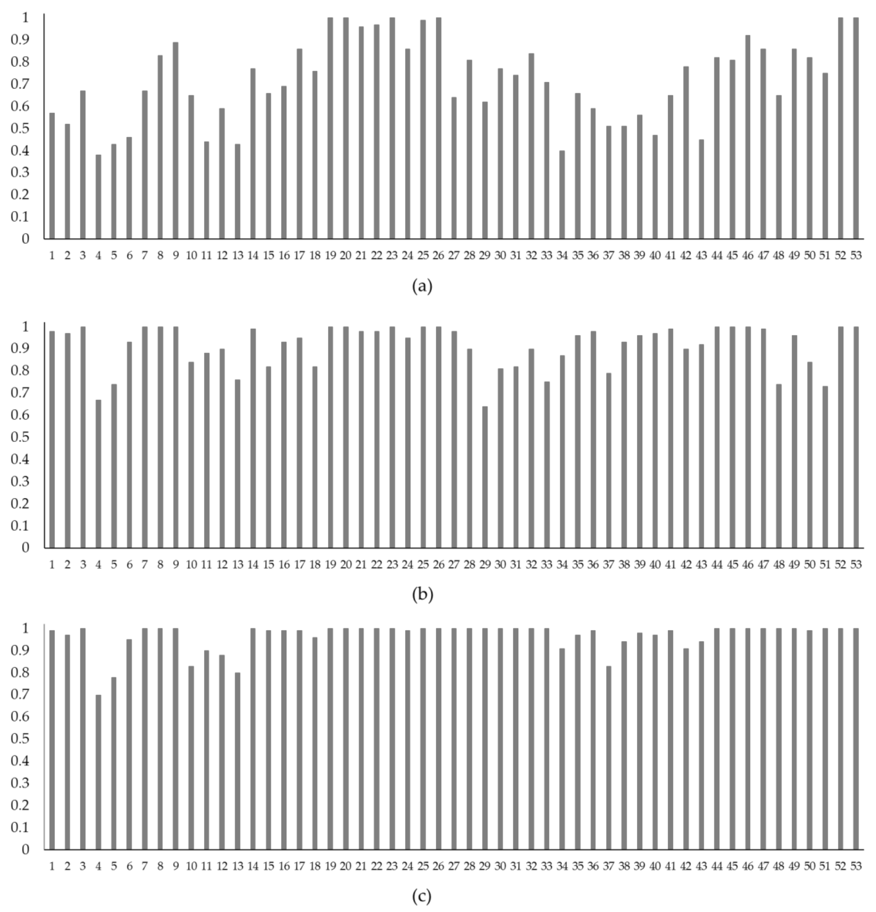
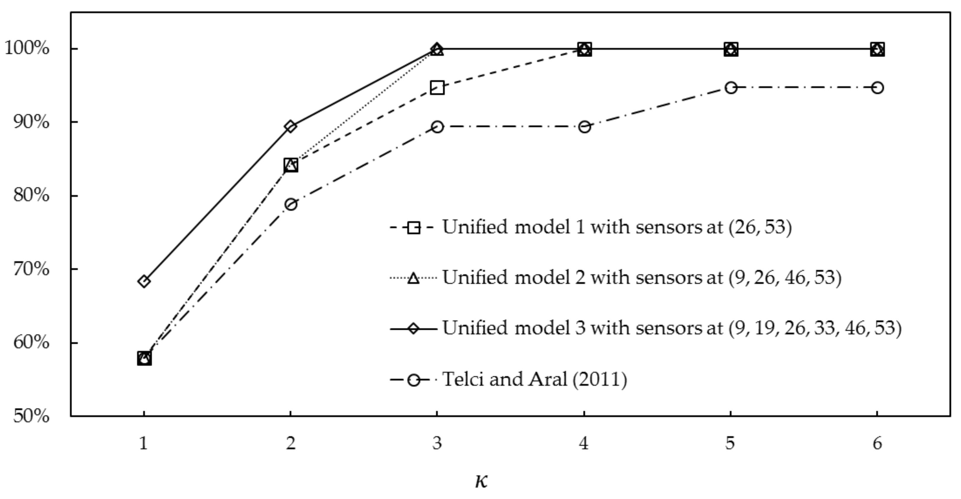
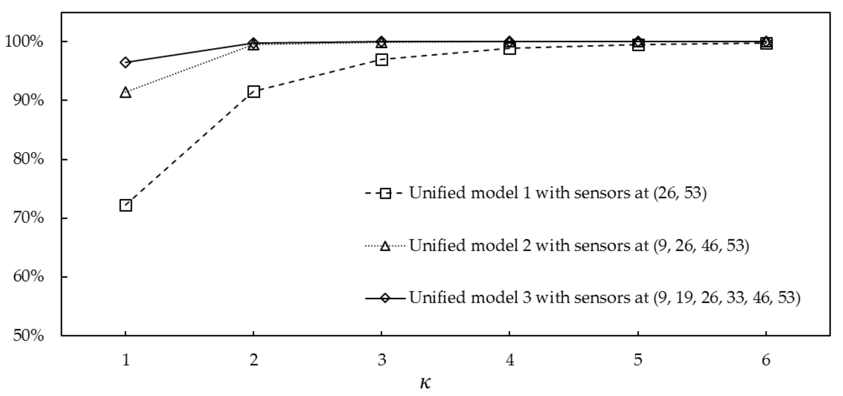
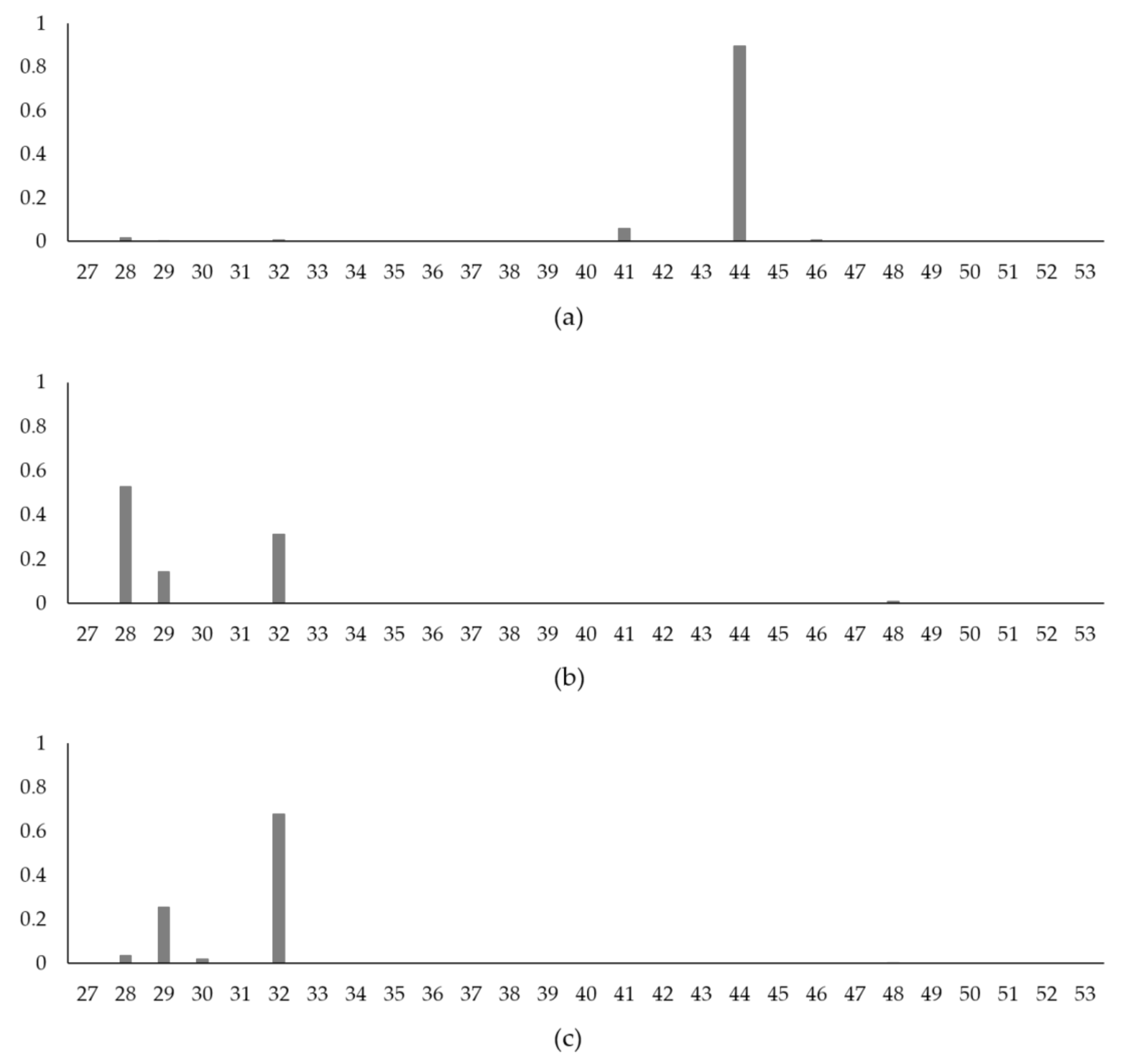
4.3. Model Assessment 1: Spill at a Candidate Location

To evaluate the performance of our unified classification model, we first tested our models on the case that a single instantaneous spill occurs exactly at one of the candidate locations under uncertainties including the spill starting time, the spill intensity, and the rain patterns. The SWMM model was executed with the spill event at each candidate location with 100 random scenarios with spill and rainfall events, and thus the number of observations for testing our models was $53\times 100$. In Figure 10a–c, the horizontal axis represents the spill location indices, and the vertical axis represents the percentage that the location with the maximum $P^i\left(d\right)$ is exactly the same as the correct spill location. Overall, the percentages at all candidate locations become higher as the number of sensors considered in a model increases. The accuracy and robustness of unified model 3 with 6 sensors was significantly enhanced when compared with those of unified model 1 with 2 sensors. The proportions of misclassifications among the total number of test data were 28%, 8%, and 4% with unified models 1, 2 and 3, respectively.

Figure 11 shows the percentage of time that the correct spill location index was included in the top $\kappa$ locations when we ordered all candidate locations based on $P^i\left(d\right)$. Unified model 1 includes the correct spill location within the top 5 locations and unified models 2 and 3 include the correct spill location within the top 2 locations with 100% accuracy over 100 random scenarios.

4.4. Model Assessment 2: Spill Near a Candidate Location

Another part of the model assessment was designed with a spill event near candidate locations, as in Telci and Aral [15]. We selected 19 spill locations, marked as R1 to R19, as shown in Figure 12 and assessed the values of $P^i\left(d\right)$ for all $d\in D$. In this assessment, both the nearest upstream and downstream locations from the spill location were accepted as the correct spill location. Figure 13 shows the percentage that any of the correct spill locations were included in the top $\kappa$ locations under decreasingly ordered $P^i\left(d\right)$. All unified models performed better than the model in Telci and Aral [15]. Obviously, higher percentages of correct identifications were achieved if more sensors were installed.

As described in Telci and Aral [15], it is difficult to recognize the correct spill location with respect to R13 because the base flow from location index 32 is much smaller than the discharged flow from location index 33 in the hydrodynamics simulation. This is the main reason that the model in Telci and Aral [15] cannot achieve 100% accuracy for spill location R13 even with an increase in $\kappa$. Figure 14a–c represent the reported values of $P^i\left(d\right)$ at candidate locations in $D_2$ from unified models 1, 2, and 3, respectively. As shown in Figure 14a, unified model 1 with two sensors cannot significantly recognize either location index 32 or 33 as the correct spill location. Nevertheless, when considering unified models 2 and 3, the value of $P^i\left(32\right)$ increases up to 0.7. Location 32 can be quantitatively identified as the correct source location based on the $P^i\left(32\right)$ values.

5. Conclusions

In this study, we proposed a framework to identify the source location of a contaminant spill, when changes in concentration levels can be observed at multiple sensors in a river system, via simulation. Specifically, the targeted river system was simulated to obtain a large data set under various random scenarios involving spill and rainfall events. To improve data-handling efficiency, the large data set was pre-processed and condensed into breakthrough curves and relative information on detection times at each pair of sensors. Random forest models were constructed and trained based on the pre-processed data. The random forest models were tested on the Altamaha river. Our model performs better than an existing model in terms of source identification. In addition, our model provides quantitative measures indicating that a selected location is the correct spill location.

We employed simulation data to test our framework in this study. Since the real data tend to include more noises in various types than the simulation data do, one may consider adopting noise-handling techniques (e.g., see Kim et al. [27]) to enhance the accuracy of our framework with real data.

Park et al. [26] presented a model to determine the best locations of sensors that minimize detection times while maintaining a certain level of detection reliability. We presented a model to identify a contaminant source location when the number and locations of sensors are given. As we have done so in this study, users may apply the method from Park et al. [26] to determine the optimal locations of sensors first, and then apply our framework to identify a source location based on the data obtained from the sensors. However, since fast contaminant detection and accurate source identification are closely related to each other and are often considered together in practical applications, a meaningful extension can be made by finding the optimal number and locations of sensors while considering detection time, detection reliability, and accuracy of source identification simultaneously. This is an ongoing work.

References

1. Gorelick, S.M.; Evans, B.; Remson, I. Identifying sources of groundwater pollution: An optimization approach. Water Resour. Res. 1983, 19, 779–790. [Google Scholar] [CrossRef]
2. Aral, M.M.; Guan, J. Genetic algorithms in search of groundwater pollution sources. In Advances in Groundwater Pollution Control and Remediation; Aral, M.M., Ed.; Springer: Dordrecht, The Netherlands, 1996; pp. 347–369. ISBN 978-94-009-0205-3. [Google Scholar]
3. Aral, M.M.; Guan, J.; Maslia, M.L. Identification of contaminant source location and release history in aquifers. J. Hydrol. Eng. 2001, 6, 225–234. [Google Scholar] [CrossRef]
4. Sun, A.Y.; Painter, S.L.; Wittmeyer, G.W. A robust approach for iterative contaminant source location and release history recovery. J. Contam. Hydrol. 2006, 88, 181–196. [Google Scholar] [CrossRef] [PubMed]
5. Singh, R.M.; Datta, B. Identification of groundwater pollution sources using GA-based linked simulation optimization model. J. Hydrol. Eng. 2006, 11, 101–109. [Google Scholar] [CrossRef]
6. Neupauer, R.M.; Lin, R. Identifying sources of a conservative groundwater contaminant using backward probabilities conditioned on measured concentrations. Water Resour. Res. 2006, 42, W03424. [Google Scholar] [CrossRef]
7. Neupauer, R.M.; Wilson, J.L. Numerical implementation of a backward probabilistic model of ground water contamination. Groundwater 2004, 42, 175–189. [Google Scholar] [CrossRef]
8. Sun, A.Y. A robust geostatistical approach to contaminant source identification. Water Resour. Res. 2007, 43. [Google Scholar] [CrossRef]
9. Singh, R.M.; Datta, B.; Jain, A. Identification of unknown groundwater pollution sources using artificial neural networks. J. Water Resour. Plan. Manag. 2004, 130, 506–514. [Google Scholar] [CrossRef]
10. Singh, R.M.; Datta, B. Artificial neural network modeling for identification of unknown pollution sources in groundwater with partially missing concentration observation data. Water Resour. Manag. 2007, 21, 557–572. [Google Scholar] [CrossRef]
11. Srivastava, D.; Singh, R.M. Breakthrough curves characterization and identification of an unknown pollution source in groundwater system using an artificial neural network (ANN). Environ. Forensics 2014, 15, 175–189. [Google Scholar] [CrossRef]
12. Boano, F.; Revelli, R.; Ridolfi, L. Source identification in river pollution problems: A geostatistical approach. Water Resour. Res. 2005, 41, W07023. [Google Scholar] [CrossRef]
13. Chen, Y.; Zhao, K.; Wu, Y.; Gao, S.; Cao, W.; Bo, Y.; Shang, Z.; Wu, J.; Zhou, F. Spatio-temporal patterns and source identification of water pollution in Lake Taihu (China). Water 2016, 8, 86. [Google Scholar] [CrossRef]
14. Ghane, A.; Mazaheri, M.; Samani, J.M.V. Location and release time identification of pollution point source in river networks based on the backward probability method. J. Environ. Manag. 2016, 180, 164–171. [Google Scholar] [CrossRef] [PubMed]
15. Telci, I.T.; Aral, M.M. Contaminant source location identification in river networks using water quality monitoring systems for exposure analysis. Water Qual. Expo. Health 2011, 2, 205–218. [Google Scholar] [CrossRef]
16. Grubner, O. Interpretation of asymmetric curves in linear chromatography. Anal. Chem. 1971, 43, 1934–1937. [Google Scholar] [CrossRef]
17. Jiang, H. Adaptive Feature Selection in Pattern Recognition and Ultra-Wideband Radar Signal Analysis; California Institute of Technology: Ann Arbor, MI, USA, 2008; ISBN 978-1-2674-8642-4. [Google Scholar]
18. Rossman, L.A. Storm Water Management Model User’s Manual, Version 5.0; U.S. Environmental Protection Agency: Cincinnati, OH, USA, 2004.
19. Telci, I.T.; Nam, K.; Guan, J.; Aral, M.M. Optimal water quality monitoring network design for river systems. J. Environ. Manag. 2009, 90, 2987–2998. [Google Scholar] [CrossRef] [PubMed]
20. Breiman, L. Random forests. Mach. Learn. 2001, 45, 5–32. [Google Scholar] [CrossRef]
21. James, G.; Witten, D.; Hastie, T.; Tibshirani, R. An Introduction to Statistical Learning: With Applications in R; Springer: New York, NY, USA, 2013; ISBN 978-1-4614-7138-7. [Google Scholar]
22. Ho, T.K. The random subspace method for constructing decision forests. IEEE Trans. Pattern Anal. Mach. Intell. 1998, 20, 832–844. [Google Scholar] [CrossRef]
23. Bernard, S.; Heutte, L.; Adam, S. Influence of hyperparameters on random forest accuracy. In Multiple Classifier Systems; Benediktsson, J.A., Kittler, J., Roli, F., Eds.; Springer: Berlin, Germany, 2009; pp. 171–180. ISBN 978-3-642-02326-2. [Google Scholar]
24. Feng, Q.; Liu, J.; Gong, J. Urban flood mapping based on unmanned aerial vehicle remote sensing and random forest classifier—A case of Yuyao, China. Water 2015, 7, 1437–1455. [Google Scholar] [CrossRef]
25. Breiman, L. Manual on Setting up, Using, and Understanding Random Forests V3.1; University of California at Berkeley: Berkeley, CA, USA, 2002. [Google Scholar]
26. Park, C.; Telci, I.T.; Kim, S.-H.; Aral, M.M. Designing an optimal water quality monitoring network for river systems using constrained discrete optimization via simulation. Eng. Optim. 2014, 46, 107–129. [Google Scholar] [CrossRef]
27. Kim, S.-H.; Aral, M.M.; Eun, Y.; Park, J.J.; Park, C. Impact of sensor measurement error on sensor positioning in water quality monitoring networks. Stoch. Environ. Res. Risk Assess. 2017, 31, 743–756. [Google Scholar] [CrossRef]
Figure 1. Schematic diagram of the problem.
Water 10 00391 g001
Figure 2. Workflow of the proposed framework.
Water 10 00391 g002
Figure 3. Example of non-zero Y t i ( z j ) over time.
Water 10 00391 g003
Figure 4. Schematic flow diagram of generating a random forest model.
Water 10 00391 g004
Figure 5. Example of a tree classifier for z = ( 9 , 19 , 26 ) .
Water 10 00391 g005
Figure 6. Overall structure of the combined classifier for the source location identification.
Water 10 00391 g006
Figure 7. Shape of the Altamaha river [19].
Water 10 00391 g007
Figure 8. Candidate locations of a spill event and of sensor locations [15].
Water 10 00391 g008
Figure 9. Unified classification model with random forest models Φ 1 ( z 1 ) and Φ 2 ( z 2 ) .
Water 10 00391 g009
Figure 10. Percentage that the location with the maximum P i ( d ) is identical to the correct spill location: (a) unified model 1 with 2 sensors at (26, 53); (b) unified model 2 with 4 sensors at (9, 26, 46, 53); and (c) unified model 3 with 6 sensors (9, 19, 26, 33, 46, 53).
Water 10 00391 g010
Figure 11. Percentage that the correct spill location is included by the top κ locations with respect to the ranking of the value P i ( d ) .
Water 10 00391 g011
Figure 12. The 19 spill locations (from R1 to R19) near candidate locations [15].
Water 10 00391 g012
Figure 13. Percentage in which the correct spill location is included by the top κ with respect to P i ( d ) .
Water 10 00391 g013
Figure 14. Values of P i ( d ) at location indices from 27 to 53 under realization R13: (a) unified model 1 with 2 sensors at (26, 53); (b) unified model 2 with 4 sensors at (9, 26, 46, 53); and (c) unified model 3 with 6 sensors (9, 19, 26, 33, 46, 53).
Water 10 00391 g014