EmiStatR: A Simplified and Scalable Urban Water Quality Model for Simulation of Combined Sewer Overflows

Abstract

Many complex urban drainage quality models are computationally expensive. Complexity and computing times may become prohibitive when these models are used in a Monte Carlo (MC) uncertainty analysis of long time series, in particular for practitioners. Computationally scalable and fast “surrogate” models may reduce the overall computation time for practical applications in which often large data sets would be needed otherwise. We developed a simplified semi-distributed urban water quality model, EmiStatR, which brings uncertainty and sensitivity analyses of urban drainage water quality models within reach of practitioners. Its lower demand in input data and its scalability allow for simulating water volume and pollution loads in combined sewer overflows in several catchments fast and efficiently. The scalable code implemented in EmiStatR reduced the computation time significantly (by a factor of around 24 when using 32 cores). EmiStatR can be applied efficiently to test hypotheses by using MC uncertainty studies or long-term simulations.

1. Introduction

Urban stormwater models are primary components of the monitoring system for real-time water flow and water quality simulation and prediction. In the literature, many urban hydrology models are well-established. However, there are few studies that attempt to model both flow and water quality taking into account the whole complexity of the physical, chemical, and biological processes involved [1,2]. Moreover, urban water quality studies need to combine hydrological modelling of natural surfaces with the performance of urban man-made structures and impervious areas in a comprehensive hydrological modelling approach. The importance of access to and preservation of clean water is emphasised by the United Nations Sustainable Development Goals to “ensure availability and sustainable management of water and sanitation for all” (Goal 6) and to “conserve and sustainably use the oceans, seas and marine resources for sustainable development” (Goal 14) [3].

Zoppou [4] presents a review of eight urban stormwater models specifically designed for simulating water quantity and quality: among others, Quantity–Quality Simulation (QQS) [5]; Storm Water Management Model (SWMM) [6]; and MIKE-SWMM, a combination of MIKE 11 [7] and SWMM. Although QQS can simulate chemical oxygen demand (COD) and total nitrogen, it does not provide the capability to simulate ammonium (NH${}_4$). Similarly, the reviewed SWMM version does not provide a routine for simulating COD or NH${}_4$. Additionally, although MIKE-SWMM simulates several water quality variables, it does not provide for specific simulation of COD.

Mitchell et al. [8] present a state-of-art review of integrated urban drainage models, in which a detailed review of seven models was conducted: Aquacyle [9], Hydro Planner [10], Krakatoa [11], UrbanCycle [12], Mike Urban [13], UVQ [14], and WaterCress [15]. Mitchell et al. [8] concluded that these models are weak in terms of handling temporal and spatial scales, input data uncertainty, and representation of urban infrastructure dynamics over time within a 10 to 100 year horizon.

Bach et al. [16] present a critical review of integrated urban drainage modelling (UDM) and compared 20 different software tools used for integrated modelling: among others, integrated urban drainage models (IUDMs) such as InfoWorks CS [17], Simulation of Biological Wastewater Systems (SIMBA) [18], SWMM [19], and WEST [20]; integrated urban water cycle models (IUWCMs) such as City Drain 3 [21], Model for Urban Stormwater Improvement Conceptualisation (MUSIC) [22], MIKE URBAN [23], UrbanCycle [12], and UrbanDeveloper [24]; and integrated urban water system models (IUWSMs) such as Dynamic Adaptation for eNabling City Evolution for Water (DAnCE4Water) [25]. In their comparison, they evaluated nine different urban drainage processes, five urban drainage components, and eight types of model applications. As a future outlook of integrated urban water models, they highlight that improvements are required for representing spatial and temporal processes in these models [8], with special attention required to address long-time-series simulation [1,26]. Additionally, they recognise that integrated urban water modelling must explore parallel computing with efforts to improve the performance of existing software [21,27] and encouraged researchers to be adaptive to the emerging computational technology. The review above suggests that there is still room to improve urban water models, specifically in the case of urban drainage models. One of the problems is that most models are very complex and require a large amount of data for calibration and to simulate processes accurately. Following [28], these complex mechanistic models describe the flow routing in pipes by the de Saint-Venant equations, which are based on the conservation of mass and momentum. These partial differential equations are solved by numerical algorithms that are often computationally demanding. Therefore, this approach is impractical for long-term simulation or optimisation tasks. As an alternative, surrogate models are frequently mentioned in the literature [28,29,30,31,32]. These models are faster and represent an approximate substitute of the “real process”, that is, the complex mechanistic model that better represents reality. Meirlaen et al. [28] distinguish between two types of possible simplifications, the empirical (black box) and the mechanistic (white box) approaches, and present a framework for developing a mechanistic surrogate model from a complex mechanistic model (CMM), reducing the computational time by a factor of 3.

Jin [33] presents a comprehensive survey of fitness approximation in evolutionary computation, whereby polynomials, the kriging model, neural networks, and support vector machines are described as the most often used methods of surrogate modelling to improve computational efficiency. However, these methods are of the black box type, which implies that the physical description and meaning of the processes that are simulated are lost.

From a different perspective, efforts have been made to simplify CMMs [34,35,36,37,38,39], but these approaches remain complex. Complex urban drainage models can be even more troublesome when Monte Carlo (MC) based uncertainty propagation analysis is required, because this analysis requires formidable computation times. Therefore, it becomes increasingly important to address scalability issues [27]. By scalability, we refer to the capability to deploy adaptive algorithms and run models efficiently in different hardware configurations (i.e., the number of threads) in distributed computing environments. Parallel computation is a key component in hydrological modelling for expediting computations.

To the best knowledge of the authors, in the realm of urban drainage modelling, there are only a few examples of scalable implementations for solving intensive computational tasks in watershed-distributed or semi-distributed modelling. Some examples of parallel computing are found in other fields, such as in the application of watershed-distributed eco-hydrological models [40] and in large-scale integrated hydrological modelling [41,42], but examples in the urban drainage domain are very scarce [27,43,44].

The above indicates that urban drainage modelling still requires simplified or surrogate models and implementations of parallel computing, specifically scalable frameworks, that are, in addition, easily accessible. In this paper, we address this need by developing and presenting EmiStatR, “Emissions and Statistics in R for Wastewater and Pollutants in Combined Sewer Systems”, a mechanistic simplified urban water model for the simulation of Combined sewer overflow (CSO) emissions. Specifically, we contribute with a tool for performing short- and long-term simulations, developed in a parallel computing framework and allowing fast calculations while preserving the physical description and meaning of the processes simulated.

We also demonstrate that it is possible to obtain similar accuracy for water quantity and quality with this simplified and scalable model, compared to results of a complex mechanistic full hydrodynamic model. We focus on COD and NH${}_4$ as water quality measures. COD is a standard for dimensioning CSO structures. NH${}_4$ represents a diluted substance that can have a significant impact on surface water quality because of possible transformation to ammonia (NH${}_3$). Additionally, COD and NH${}_4$ are key variables for evaluation of the performance of wastewater treatment plants (WwTPs) and the quality status of receiving water bodies. A detailed outlook regarding the relevance of transformation and nutrient removal from the water column is presented by Bell and co-workers [45].

This paper has three main objectives: (1) The development of a simplified mechanistic urban water model, EmiStatR, which represents the overall dynamic behaviour of the CSO spill volume, load, and concentration of COD and NH${}_4$. (2) The presentation of an implementation of the model in R with parallel computation capabilities, allowing fast and scalable calculations, particularly for scenarios with long simulation periods and in MC uncertainty propagation mode. (3) The calibration and application of EmiStatR to a Luxembourg case study and validation by comparing the performance against a CMM that uses the de Saint-Venant partial differential equations to describe the flow routing in the pipes of the sewer network.

2. Methods

EmiStatR targets the simulation of CSO emissions of pollutants to the receiving water body, in terms of indicator variables, such as COD and NH${}_4$. In this section, we describe the conceptual and mathematical model and its implementation in R.

2.1. Conceptual Model

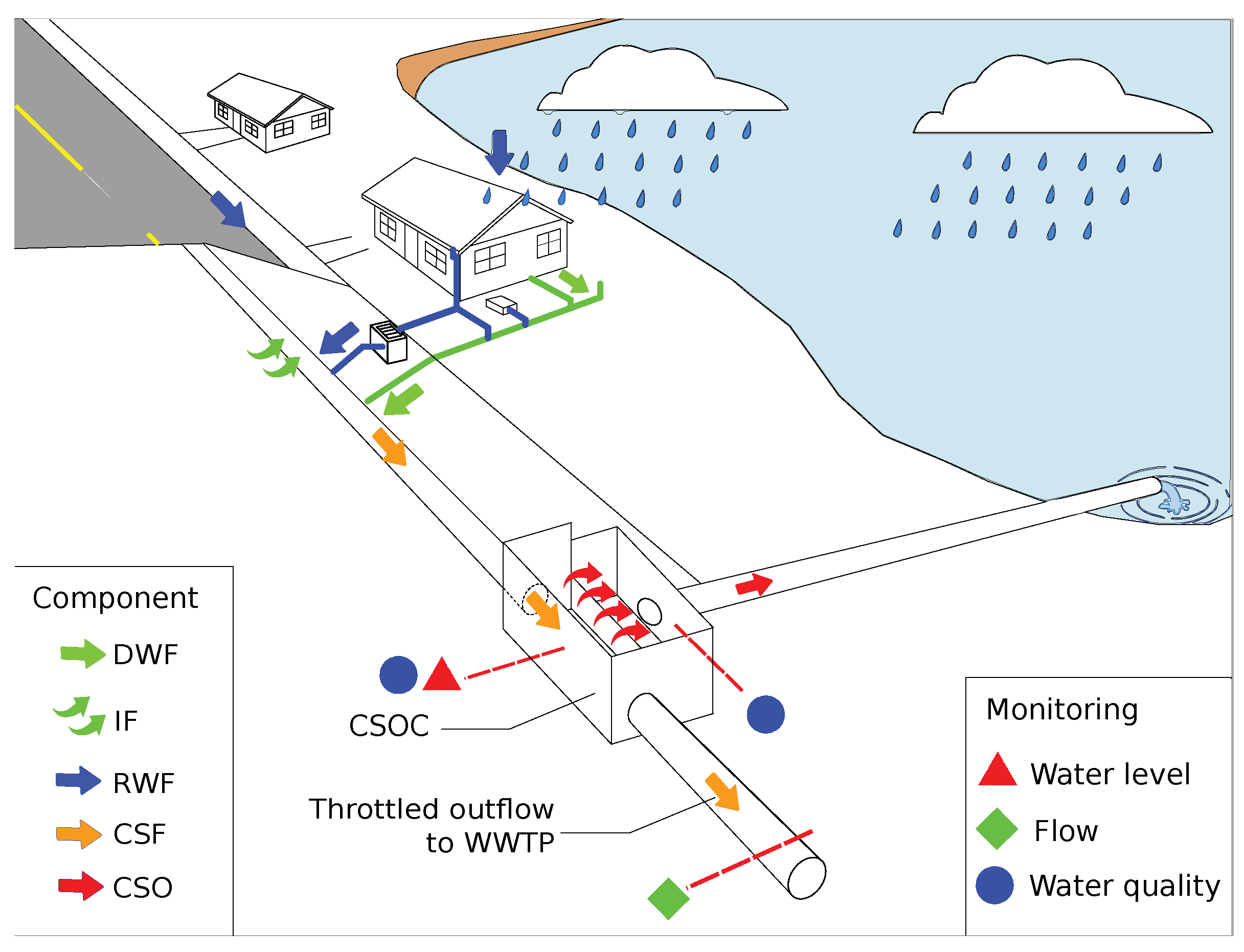
The EmiStatR model includes six main components to simulate combined sewage discharges of a catchment (Figure 1):

• Dry weather flow (DWF): EmiStatR assumes a constant DWF resulting from specific water consumption per population equivalent (PE) and a specific discharge of infiltration inflow per hectare of contributing impervious area to combined sewage flow (CSF).
• Pollution of DWF: This is the specific load contribution per PE and day of COD and NH${}_4$. No pollutant contribution of infiltration inflow is taken into account.
• Rain weather flow (RWF): This is the total run-off of rainfall on the impervious catchment area contributing to CSF. The RWF is discharged in a specific flow time ($t_{\mathit{fS}}$) to the sewer outlet or CSO structures downstream from the catchment; that is, the flow time in the sub-catchment ($t_{\mathit{fS}}$) is a parameter of calibration.
• Pollution of RWF: Constant surface run-off concentrations of COD and NH${}_4$ are assumed. EmiStatR further assumes the complete mixing of pollutants in simultaneously flowing volume components and CSO chamber (CSOC) structures.
• CSF and pollution: These are the sum of the DWF and RWF for the CSF and the consequent pollution load.
• CSO volume and pollution: These are the volume diverted towards the receiving water body that is produced when the overflow or spill weir level in the CSOC is exceeded and the pollution measured as COD and NH${}_4$ loads.

As shown in Figure 1, the sewer system under investigation includes a CSOC structure to store first-flush pollutant peaks. After filling of the storage capacity, the excess volume and pollutant inflows are discharged through a combined sewage spill structure. The excess flow and pollutant load are not conveyed to the WwTP but are diverted directly to the receiving water (i.e., the environment).

In EmiStatR a simple volume balance taking into account inflow volume, present storage capacity, and outflow to the WwTP is implemented to simulate the CSOC structure. In case of a spill, the pollutant concentrations in the CSO are equivalent to the combined sewage inflow concentrations of the structure.

At the CSOC structure, a simple volume balancing takes place: (1) Substance and volume flows are stored and discharged to the WwTP if the storage volume is not completely filled up. (2) If the storage volume is completely filled up, the proportion of the volume inflow that is not discharged to the WwTP goes to the CSO.

2.2. Governing Equations

2.2.1. Dry Weather Flow

The DWF, $Q_{s24}$ $(\mathrm{L}·{\mathrm{s}}^{-1})$, is the product of the residential wastewater flow per PE, $\mathit{qs}$, and the PEs connected to the CSO structure, ${\mathit{pe}}_i$. The time series $\mathit{qs}$ may follow a daily pattern given by a technical association for wastewater and water management but may also be a user-defined daily or weekly pattern, thus allowing different parts of the week to be differentiated between, for example, weekdays and weekends. Moreover, seasonal patterns can be defined to account for differences between months or seasons. The time series of PEs ${\mathit{pe}}_i$ can also vary over time to account for differences between weekdays and weekends or for seasonal effects, such as because of tourism. The time series $\mathit{qs}$ and ${\mathit{pe}}_i$ are of lengths equal to that of the rainfall time series, $P_{\mathit{1}}$ (see Section 2.2.3). The DWF is calculated as

$${Q_{s24}}_i=\frac{1}{86,400}·{\mathit{pe}}_i·{\mathit{qs}}_i,$$

(1)

where

• $i$ is the ith term of the time series (−),
• $\mathit{pe}$ are the PEs of the connected CSO structure at time i (PE),
• $\mathrm{PE}$ is the units for PEs (unit per capita loading), and
• $\mathit{qs}$ is the individual water consumption at time i (residential) $(\mathrm{L}·{\mathrm{PE}}^{-1}·{\mathrm{day}}^{-1})$.

We note that $pe$ refers to the time series of PEs with units PE. The number 86,400 is a factor for unit conversion (from days to seconds). The infiltration flow, $Q_f$ $(\mathrm{L}·{\mathrm{s}}^{-1})$, is computed as

$${Q_f}_i=A_{\mathit{imp}}·{q_f}_i,$$

(2)

where

• $A_{\mathit{imp}}$ is the impervious area of the catchment (ha), and
• $q_f$ is the specific infiltration water inflow at time i $(\mathrm{L}·{\mathrm{s}}^{-1}·{\mathrm{ha}}^{-1})$.

Consequently, the total DWF, $Q_{t{24}_i}$ $(\mathrm{L}·{\mathrm{s}}^{-1})$, is calculated as

$${Q_{t24}}_i={Q_{s24}}_i+{Q_f}_i.$$

(3)

The contribution of DWF to the combined sewage volume during a time interval $\Delta t\left(\min \right)$ is called the “dry weather volume” (amount of dry weather water in CSF), $V_{\mathit{dw}}$ (m${}^3$):

$${V_{\mathit{dw}}}_i=0.06·\Delta t·{Q_{t24}}_i.$$

(4)

The number 0.06 is a factor for unit conversion (from minutes to seconds and from litres to cubic metres).

2.2.2. DWF Pollutants

The time series of two dry weather pollutant concentrations are calculated: the COD concentration, $C_{\mathit{COD}}$ $(\mathrm{mg}·{\mathrm{L}}^{-1})$, and the NH${}_4$ concentration, $C_{\mathit{NH}\mathit{4}}$ $(\mathrm{mg}·{\mathrm{L}}^{-1})$. These are time series with length equal to $P_{\mathit{1}}$ and that make use of $C_{\mathit{COD},S}$ and $C_{\mathit{NH}\mathit{4},S}$, which are assumed to be constant:

$${C_{\mathit{COD}}}_i=\frac{{10}^3·{\mathit{pe}}_i·C_{\mathit{COD},S}}{{\mathit{qs}}_i·p{e}_i+86,400·A_{\mathit{imp}}·q_{f_i}},$$

(5)

$${C_{\mathit{NH}\mathit{4}}}_i=\frac{{10}^3·{\mathit{pe}}_i·C_{\mathit{NH}\mathit{4},S}}{{\mathit{qs}}_i·p{e}_i+86,400·A_{\mathit{imp}}·q_{f_i}},$$

(6)

where

• $C_{\mathit{COD},S}$ is the COD sewage pollution per capita (PE) load per day (g·PE⁻¹·day⁻¹), and
• $C_{\mathit{NH}\mathit{4},S}$ is the NH₄ sewage pollution per capita (PE) load per day (g·PE⁻¹·day⁻¹).

2.2.3. Rain Run-Off Volume and Rain Weather Flow

The contribution of rainwater to the combined sewage volume is called the “rainwater volume”, $V_r$ (m${}^3$). This is a vector whose length is equal to that of $P_{\mathit{1}}$. $P_{\mathit{1}}$ is delayed by $t_{\mathit{fS}}$ time steps that represent a delay in time response related to flow time in the sewer system. The parameter $t_{\mathit{fS}}$ may be calibrated with observed data. The rainwater volume accumulated during a time interval $\Delta t\left(\min \right)$ is computed as

$${V_r}_i=10·{{P_{\mathit{1}}}_{i-t}}_{\mathit{fS}}·[C_{imp}·A_{imp}+C_{per}(A_{total}-A_{imp})],$$

(7)

where

• $P_{\mathit{1}}$ is the rainfall depth per time step ($\Delta t$) at time i$\left(\mathrm{mm}\right)$,
• $A_{\mathit{imp}}$ is the impervious area of the catchment (ha),
• $A_{\mathit{total}}$ is the total area of the catchment (ha),
• $C_{imp}$ is the run-off coefficient for impervious areas (−), and
• $C_{per}$ is the run-off coefficient for pervious areas (−).

2.2.4. Combined Sewage Flow

The calculation of the CSF is done by introducing the concept of the “combined sewage mixing ratio”, ${\mathit{cs}}_{\mathit{mr}}$ (–). This is the ratio between $V_{\mathit{dw}}$ and $V_r$:

$${\mathit{cs}}_{\mathit{mri}}=\left\{\begin{array}{c}\begin{array}{cc}0,\hfill & \mathrm{if}{V_r}_i\le ϵ,\hfill \\ \frac{V_{d{w}_i}}{{V_r}_i},\hfill & \mathrm{if}{V_r}_i>ϵ,\hfill \end{array}\hfill \end{array}\right.$$

(8)

where

• $ϵ$ is the precision term equal to ${10}^{-5}$ (–).

2.2.5. CSO Volume

The calculation of the CSO volume is based on the excess volume stored in the Combined sewer overflow chamber (CSOC). The volume in the CSOC is calculated from the curve water level versus water volume. This requires that an initial water level in the CSOC, $Le{v}_{ini}$ (m), is provided by the user. The throttled outflow or pass-forward flow of the CSOC, $Q_d$, conveyed towards the WwTP is defined by the discharge of the CSOC by an orifice:

$$Q_{di}=\left\{\begin{array}{c}\begin{array}{cc}{10}^3·C_d·A_d{\left(2·g·Le{v}_{ini}\right)}^{0.5}\hfill & \mathrm{if}i=1,\hfill \\ {10}^3·C_d·A_d{\left(2·g·Le{v}_i\right)}^{0.5}\hfill & \mathrm{if}i>1,\hfill \end{array}\hfill \end{array}\right.$$

(9)

where

• $Q_d$ is the throttled outflow to the WwTP $(\mathrm{L}·{\mathrm{s}}^{-1})$;
• $C_d$ is the orifice coefficient of discharge (−);
• $A_d$ is the orifice area ($\pi ·D_d^2/4$) $\left({\mathrm{m}}^2\right)$;
• g is the gravitational acceleration, 9.81 m$·{\mathrm{s}}^{-2}$; and
• $Lev$ is the water level in the CSOC (m).

After computation of $Q_d$, it is checked whether the value obtained is below the maximum throttled outflow, $Q_{d,max}$(L·s⁻¹), defined by the user:

$${Q_d}_i=\left\{\begin{array}{c}\begin{array}{cc}{Q_d}_i\hfill & \mathrm{if}{Q_d}_i<Q_{d,max},\hfill \\ Q_{d,max}\hfill & \mathrm{if}{Q_d}_i\ge Q_{d,max}.\hfill \end{array}\hfill \end{array}\right.$$

(10)

Four stages of the CSOC for calculation of the CSO volume are defined: (1) Filling up, characterised by the CSOC filling up volume, $V_{\mathit{Chamber}}$, of the CSOC; (2) CSO, characterised by the completely filled CSOC volume, $V_{\mathit{Chamber}}$, being equal to the volume of the CSOC; (3) stagnation: Characterised by the CSOC filling up volume, $V_{\mathit{Chamber}}$, of the CSOC being equal to zero; (4) emptying: Characterised by the CSOC filling up volume, $V_{\mathit{Chamber}}$, of the CSOC. A status variable is defined to determine when the CSOC is filling up:

$$o_{{\mathit{cfyn}}_i}=\left\{\begin{array}{c}\begin{array}{cc}1\hfill & \mathrm{if}\left({V_r}_i+V_{{\mathit{dw}}_i}\right)>{V_d}_i,\hfill \\ 0\hfill & \mathrm{if}\left({V_r}_i+V_{{\mathit{dw}}_i}\right)\le {V_d}_i,\hfill \end{array}\hfill \end{array}\right.$$

(11)

with

$$V_{d_i}=0.06·\Delta t·Q_{d_i},$$

(12)

and where

• $o_{\mathit{cfyn}}$ is the status variable for the CSOC filling up or spilling out (1—filling up; 0—spilling out) $(-)$,
• $V_d$ is the volume of throttled outflow to the WwTP at time i $\left({\mathrm{m}}^3\right)$, and
• $Q_d$ is the throttled outflow to the WwTP at time i $(\mathrm{L}·{\mathrm{s}}^{-1})$.

After checking whether the CSOC is filling up or not, the volume $V_{\mathit{Chamber}}$ $\left({\mathrm{m}}^3\right)$ is calculated:

$${V_{\mathit{Chamber}}}_i=\{\begin{array}{c}0\mathrm{if}i=1,\hfill \\ \underset{\mathrm{filling}\mathrm{up}}{\underbrace{{V_{\mathit{Chamber}}}_{i-\mathit{1}}+\Delta V_i\mathrm{if}\left(o_{\mathit{cfyn}}=1\right)\wedge \left[{V_{\mathit{Chamber}}}_{i-\mathit{1}}<\left(V-\Delta V_i\right)\right]}},\hfill \\ \underset{\mathrm{spill}}{\underbrace{V\mathrm{if}\left(o_{\mathit{cfyn}}=1\right)\wedge \left[{V_{\mathit{Chamber}}}_{i-\mathit{1}}\ge \left(V-\Delta V_i\right)\right]}},\hfill \\ \underset{\mathrm{stagnation}}{\underbrace{0\mathrm{if}\left(o_{\mathit{cfyn}}=0\right)\wedge \left[\left({V_{\mathit{Chamber}}}_{i-\mathit{1}}+\Delta V_i\right)\le ϵ\right]}},\hfill \\ \underset{\mathrm{emptying}}{\underbrace{{V_{\mathit{Chamber}}}_{i-\mathit{1}}+\Delta V_i\mathrm{if}\left(o_{\mathit{cfyn}}=0\right)\wedge \left[\left({V_{\mathit{Chamber}}}_{i-\mathit{1}}+\Delta V_i\right)>ϵ\right]}},\hfill \end{array}$$

(13)

with

$$\Delta V_i={V_r}_i+{V_{\mathit{dw}}}_i-V_{d_i},$$

(14)

and where

• V is the volume of the CSOC $\left({\mathrm{m}}^3\right)$.

Upon calculation of the filling up volume, the CSO spill volume, $V_{\mathit{Sv}}$ $\left({\mathrm{m}}^3\right)$, is calculated as

$${V_{\mathit{Sv}}}_i=\left\{\begin{array}{cc}\Delta V_i\hfill & \mathrm{if}{V_{\mathit{Chamber}}}_i=V,\hfill \\ {V_{Chamber}}_i-V\hfill & \mathrm{if}{V_{Chamber}}_i>V,\hfill \\ ϵ\hfill & \mathrm{if}{V_{Chamber}}_i<V.\hfill \end{array}\right.$$

(15)

2.2.6. CSO Pollutants

The spill emissions of COD and NH${}_4$ are calculated in two steps: (1) Calculation of the COD and NH${}_4$ spill loads, $B_{\mathit{COD},\mathit{Sv}}$ and $B_{\mathit{NH}\mathit{4},\mathit{Sv}}$, respectively; and (2) Calculation of the COD and NH${}_4$ spill concentrations, $C_{\mathit{COD},\mathit{Sv}}$ and $C_{\mathit{NH}\mathit{4},\mathit{Sv}}$, respectively.

$${B_{\mathit{COD},\mathit{Sv}}}_i=\left\{\begin{array}{cc}\frac{{V_{\mathit{Sv}}}_i·{c{s}_{mr}}_i}{{c{s}_{mr}}_i+1}{C_{\mathit{COD}}}_i+\frac{{V_{\mathit{Sv}}}_i}{{c{s}_{mr}}_i+1}{{\mathit{COD}}_r}_i\hfill & \mathrm{if}{V_{\mathit{Sv}}}_i>ϵ,\hfill \\ ϵ\hfill & \mathrm{if}{V_{\mathit{Sv}}}_i\le ϵ.\hfill \end{array}\right.$$

(16)

$${B_{\mathit{NH}\mathit{4},\mathit{Sv}}}_i=\left\{\begin{array}{cc}\frac{{V_{\mathit{Sv}}}_i·{c{s}_{mr}}_i}{{c{s}_{mr}}_i+1}{C_{\mathit{NH}\mathit{4}}}_i+\frac{{V_{\mathit{Sv}}}_i}{{c{s}_{mr}}_i+1}\mathit{NH}{\mathit{4}}_r\hfill & \mathrm{if}{V_{\mathit{Sv}}}_i>ϵ,\hfill \\ ϵ\hfill & \mathrm{if}{V_{\mathit{Sv}}}_i\le ϵ.\hfill \end{array}\right.$$

(17)

Here,

• $B_{\mathit{COD},\mathit{Sv}}$ is the COD load in the spill volume (g),
• ${\mathit{COD}}_r$ is the rainwater pollution∔COD concentration $(\mathrm{mg}·{\mathrm{L}}^{-1})$,
• $B_{\mathit{NH}\mathit{4},\mathit{Sv}}$ is the NH₄ load in the spill volume (g), and
• $\mathit{NH}{\mathit{4}}_r$ is the rainwater pollution—NH${}_4$ concentration $(\mathrm{mg}·{\mathrm{L}}^{-1})$.

${\mathit{COD}}_r$ can be a time series of length equal to $P_{\mathit{1}}$ or a unique value constant in time. The emissions in terms of the concentrations of COD and NH${}_4$ are calculated and make use of $C_{\mathit{COD},\mathit{Sv}}$ (mg·L⁻¹), which is defined as the ratio of $B_{\mathit{COD},\mathit{Sv}}$ and $V_{\mathit{Sv}}$. Similarly, $C_{\mathit{NH}\mathit{4},\mathit{Sv}}$ (mg·L⁻¹) is the ratio of $B_{\mathit{NH}\mathit{4},\mathit{Sv}}$ and $V_{\mathit{Sv}}$.

2.3. Model Implementation in R

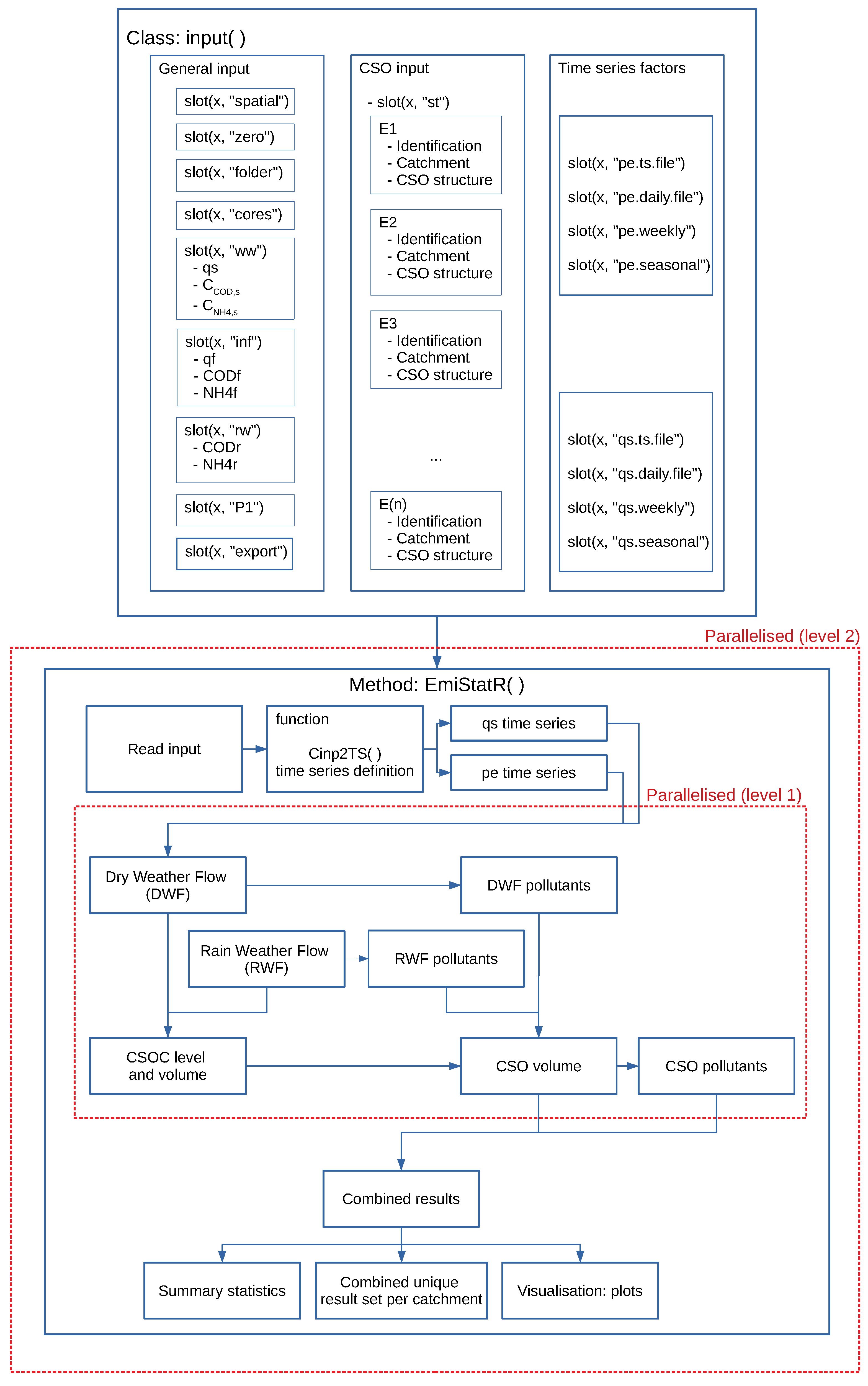
EmiStatR is available for download from the Comprehensive R Archive Network (CRAN) (https://cran.r-project.org/web/packages/EmiStatR/). This includes a user manual with several examples that can be run in R. The entire work flow for EmiStatR is illustrated in Figure 2.

2.3.1. Input Data Definition

EmiStatR is implemented in R [47] by defining a specific input() class (Figure 2). The model input data are set up in the class input() and can be grouped into three main categories (

Table 1. General and combined sewer overflow (CSO) structure input data of EmiStatR.

General Input	Units	CSO Input	Units
1. Wastewater		1. Identification
Water consumption, $\mathit{qs}$	$\mathrm{L}·{\mathrm{PE}}^{-1}·{\mathrm{day}}^{-1}$a	ID of the structure	–
Water consumption, factors b	–	Name of the structure	–
Pollution COD c, $C_{\mathit{COD},S}$	$\mathrm{g}·{\mathrm{PE}}^{-1}·{\mathrm{day}}^{-1}$
Pollution NH4 d, $C_{\mathit{NH}\mathit{4},S}$	$\mathrm{g}·{\mathrm{PE}}^{-1}·{\mathrm{day}}^{-1}$	2. Catchment data
		Name of the municipality	–
2. Infiltration water		Name of the catchment	–
Inflow, $q_f$	L· s${}^{-1}$ · ha${}^{-1}$	Number of the catchment	–
Pollution COD, CODf	$\mathrm{g}·{\mathrm{PE}}^{-1}·{\mathrm{day}}^{-1}$	Land use	–
Pollution NH${}_4$, $\mathit{NH}{\mathit{4}}_f$	$\mathrm{g}·{\mathrm{PE}}^{-1}·{\mathrm{day}}^{-1}$	Total area, $A_{\mathit{total}}$	ha
		Impervious area, $A_{\mathit{imp}}$	ha
3. Rainwater		Run-off coefficient for impervious area, $C_{imp}$	–
Precipitation time series, $P_{\mathit{1}}$	mm	Run-off coefficient for pervious area, $C_{per}$	–
Pollution COD, ${\mathit{COD}}_r$	$\mathrm{mg}·{\mathrm{L}}^{-1}$	Flow time structure, $t_{\mathit{fS}}$	time step
Pollution NH${}_4$, $\mathit{NH}{\mathit{4}}_r$	$\mathrm{mg}·{\mathrm{L}}^{-1}$	Population equivalents, ${\mathit{pe}}_i$	PE
		Population equivalents, factors b	–
		3. CSO structure data
		Volume, V	m${}^3$
		Curve level–volume, $lev2vol$	m, m${}^3$
		Initial water level, $Le{v}_{ini}$	m
		Maximum throttled outflow, $Q_{d,max}$	L· s${}^{-1}$
		Orifice diameter, $D_d$	m
		Orifice coefficient of discharge, $C_d$	–

^a Population equivalent (PE). ^b Factors for daily, weekly, and monthly patterns. ^c Chemical oxygen demand (COD). ^d Ammonium (NH₄).

, columns 1 and 2):

• Wastewater production data, that is, water consumption in PE and characterisation of the pollution load of wastewater in terms of COD and NH${}_4$ concentrations in PE.
• Run-off and specific pollutant load contribution per PE and day (COD and NH${}_4$ concentrations) of infiltration water.
• Precipitation data, that is, time series of rainfall and rainfall run-off pollution in terms of concentrations of COD and NH${}_4$.

The general input variables of the CSO structure are grouped into three main components (Table 1, columns 3 and 4):

• Identification, that is, ID and name of structure.
• Catchment data, that is, name of the municipality, name and number of the catchment, land use (residential, commercial, and industrial), total area of the catchment, impervious area, and PEs connected to the sewer system.
• CSO structure data, that is, data regarding the throttled outflow diverted to the WwTP and the total storage volume of the CSOC.

The main goal of EmiStatR is to simulate emissions of spill volume in individual CSO structures. If calibration data are available, EmiStatR parameters may be calibrated prior to simulation using the DiffeRential Evolution Adaptive Metropolis (DREAM) algorithm [48]. The DREAM algorithm is integrated through the R package dream [49]. If calibration is not feasible, the model can also be run using parameter values taken from reference literature and guidelines.

Table 2. Default values for input data of EmiStatR.

Input	Units	Reference Value	Literature Source	Range (This Study)
Wastewater
Water consumption, $\mathit{qs}$	$\mathrm{L}·{\mathrm{PE}}^{-1}·{\mathrm{day}}^{-1}$a	150 b	[50]	[130, 170]
Pollution COD c, $C_{\mathit{COD},S}$	$\mathrm{g}·{\mathrm{PE}}^{-1}·{\mathrm{day}}^{-1}$	120	[51]	[90, 150]
Pollution TKN d	$\mathrm{g}·{\mathrm{PE}}^{-1}·{\mathrm{day}}^{-1}$	11	[51]	[7, 15]
Pollution NH${}_4$ e	$\mathrm{g}·{\mathrm{PE}}^{-1}·{\mathrm{day}}^{-1}$	4.7	This study	[1, 8]
Infiltration water
Inflow, $q_f$	L· s${}^{-1}$ · ha${}^{-1}$	0.05	[52]	[0, 2]
Catchment data
Run-off coefficient for impervious area, $C_{imp}$	–	See [53]	[53]	[0.20, 095]
Run-off coefficient for pervious area, $C_{per}$	–	See [53]	[53]	[0.05, 0.50]
Flow time structure, $t_{\mathit{fS}}$	time step	2	This study	[0, 12]
CSO structure data
Initial water level, $Le{v}_{ini}$	m	$L_{max}$f/2	This study	[0, $L_{max}$]
Orifice coefficient of discharge, $C_d$	–	1.25	This study	[0.01, 2]

^a PE: Population equivalent units; ^b mean value for European countries; ^c COD: Chemical oxygen demand; ^d TKN: Total Kjeldahl nitrogen; ^e NH${}_4$: Ammonium; ^f $L_{max}$: Maximum water level in the combined sewer overflow chamber (CSOC).

provides reference values and calibration ranges for the most important EmiStatR parameters.

2.3.2. Implementation of a Scalable Approach

Because MC analysis and long-term simulations of a large number of catchments EmiStatR may be slow, we made the code more scalable through parallel computation. This was done via the R package doParallel [54], which provides a parallel back-end for the functions of the foreach package [55]. It depends on the R packages foreach, iterators [56], and parallel [47] and provides functionality for creating parallel loops through the foreach package. The doParallel package is an interface between the foreach and parallel packages of R 2.14.0 and later parallel wraps functions of the multicore [57] and snow packages [58].

The parallel package evaluates larger chunks of code in parallel. In order to complete a computational task in parallel, these chunks should be evaluated independently, should take the same length of time, and should not communicate with each other. The typical parallel computational model is the following [47]:

• Start up M “worker” processes, and do any initialisation needed for the workers.
• Send any data required for each task to the workers.
• Split the task into M roughly equally sized chunks, and send the chunks (including the R code needed) to the workers.
• Wait for all workers to complete their tasks, and collect results.
• Repeat steps 1 to 4 for any further tasks.
• Stop and close the worker processes.

In our specific case study, each of the M workers is related to a MC simulation. EmiStatR can also be parallelised for each sub-catchment to address scalability. An example is given in the EmiStatR package documentation. How the parallelisation is integrated into the entire workflow is illustrated in Figure 2, where parallelisation is set in the input() class, slot(x, “cores”). Level 1 indicates the parallel computation done inside EmiStatR. Level 2 indicates the parallel computation done outside of EmiStatR, for example, MC simulations or optimisation, in other R packages such as dream [49] or stUPscales ([59]; under review, to be published in this issue) packages.

3. Case Study

3.1. Study Area

A test case was created to evaluate the use and performance of EmiStatR. A sub-catchment of the Haute-Sûre catchment in the northwest of Luxembourg was chosen. The combined sewer system of the sub-catchment drains the three villages Goesdorf, Kaundorf, and Nocher-Route. In the local sewer system downstream from the villages, three CSOCs are located to store pollutant peaks in the first flush of CSFs. Figure 3 depicts their locations and the delineation of the catchment. The topography of the area is characterised by a hilly landscape. The elevations around Goesdorf are between 390 and 490 m, around Kaundorf are between 370 and 464 m, and in the area of Nocher-Route vary between 400 and 485 m. The main land use types in the villages are residential, smaller industries, and farms. Outside of the villages, forest as well as agricultural areas and grassland are the dominating land uses. The receiving water bodies at CSO structures in Goesdorf, Kaundorf, and Nocher-Route are tributaries of the river Sûre (Sauer, in German) (Figure 3).

3.2. Model Calibration

Measured precipitation time series at the Goesdorf CSOC served as input for the model calibration for water quantity output variables. This time series was recorded from May 15, 2011 to June 3, 2011 at 1 min resolution. Seven water quantity parameters were selected for calibration: (1) Water consumption, $qs$; (2) infiltration flow, $q_f$; (3) time flow, $t_{fS}$; (4) run-off coefficient for impervious area, $C_{imp}$; (5) run-off coefficient for pervious area, $C_{per}$; (6) orifice coefficient of discharge, $C_d$; and (7) initial level of water in the CSOC, $Le{v}_{ini}$.

For calibration, we used the DREAM algorithm [48]. DREAM has the capability of running and evaluating multiple different chains simultaneously for global exploration. The algorithm tunes the proposal distribution in randomised subspaces during the search. DREAM enhances the applicability of Markov chain Monte Carlo (MCMC) sampling approaches in complex problems [48]. The main building block of the DREAM algorithm is the Differential Evolution Markov Chain (DE-MC) method presented by ter Braak [60]. In DE-MC, different Markov chains are run simultaneously in parallel. At the current time, they form a population. Jumps in each chain are generated by taking a fixed multiple of the difference of two random chains without replacement. To accept or reject candidate points, the Metropolis ratio is used [60].

The DREAM algorithm is implemented in R in the R package dream [49]. Observations of water level in the Goesdorf storage CSOC served as reference for optimising the model parameters. The water level was recorded from April 19, 2011 to July 15, 2011 at 30 s time steps. The precipitation and water level observations were aggregated to 10 min intervals to assure that the model simulations and observations had the same temporal support before comparison. The observations were divided into two sets, one for calibration and one for validation. The calibration set comprised the initial section of the measurements from May 15 to June 3, 2011, a total of 2698 records at 10 min time steps. The validation set comprised the measurements from June 3 to July 7, 2011, a total of 4901 records at 10 min time steps.

DREAM optimises by minimising the root-mean-squared error (RMSE). As accuracy measures, the calibration results were evaluated by the mean error (ME), RMSE, and the Nash–Sutcliffle model efficiency coefficient (NSE) [61]:

$$\mathrm{RMSE}=\sqrt{\frac{1}{N}\sum _{i=1}^N{(S_i-O_i)}^2},$$

(18)

$$\mathrm{ME}=\frac{1}{N}\sum _{i=1}^N(S_i-O_i),$$

(19)

$$\mathrm{NSE}=1-\frac{{\sum }_{i=1}^N{(S_i-O_i)}^2}{{\sum }_{i=1}^N{(O_i-\overline{O})}^2},$$

(20)

where

• $O_i$ is the ith observation,
• $S_i$ is the ith simulation,
• $\overline{O}$ is the mean of the observations, and
• N is the number of observations (and simulations).

For Kaundorf and Nocher-Route, sufficient calibration data were not available. We therefore used the reference values (Table 2).

Regarding the water quality module of EmiStatR, six parameters are required to define pollution in terms of the following: (1) COD load per PE per day in the wastewater, $C_{COD,S}$; (2) NH${}_4$ load per PE per day in the wastewater, $C_{NH4,S}$; (3) COD load per PE per day in the infiltration water, $CO{D}_f$; (4) NH${}_4$ load per PE per day in the infiltration water, $NH{4}_f$; (5) COD concentration in the run-off, $CO{D}_r$; and (6) NH${}_4$ concentration in the run-off, $NH{4}_r$. If these parameters are not measured directly, then they can be calibrated when observations of COD or NH${}_4$ (concentrations or loads) in the output of the CSO spill volume are available. In this case study, we did not need to calibrate $C_{COD,S}$ and $C_{NH4,S}$ for Goesdorf, Kaundorf, or Nocher-Route, because 91 observations in total under DWF conditions were available. The measured $C_{COD,S}$ had a mean value of 104 $\mathrm{g}·{\mathrm{PE}}^{-1}·{\mathrm{day}}^{-1}$ with a standard deviation of 87.5 $\mathrm{g}·{\mathrm{PE}}^{-1}·{\mathrm{day}}^{-1}$. The measured $C_{NH4,S}$ had a mean value of 4.7 $\mathrm{g}·{\mathrm{PE}}^{-1}·{\mathrm{day}}^{-1}$ with a standard deviation of 1.92 $\mathrm{g}·{\mathrm{PE}}^{-1}·{\mathrm{day}}^{-1}$. The temporal support of these observations was 120 minutes. The other input parameters of the water quality module ($CO{D}_f$, $NH{4}_f$, $CO{D}_r$, and $NH{4}_r$) were set to zero, because the concentrations in rainfall and infiltration water were judged negligible compared to that of household sewage. We chose periods from 2010 and 2011 for both calibration and validation.

Calibration Results of the Water Quantity Model

Table 3. Calibration and validation results of the hydraulic model in EmiStatR as calibrated with the DREAM algorithm (Goesdorf 2011, 10 min time step).

Parameter	Units	Range of Sampling	Calibrated Value
Water consumption, $qs$	$\mathrm{L}·{\mathrm{PE}}^{-1}·{\mathrm{day}}^{-1}$	[130, 170]	152
Infiltration flow, $q_f$	L·s${}^{-1}·$ha${}^{-1}$	[0, 0.2]	0.116
Time flow, $t_{fS}$	time step	[0, 12]	1
Run-off coefficient for impervious area, $C_{imp}$	–	[0.20, 0.95]	0.28
Run-off coefficient for pervious area, $C_{per}$	–	[0.05, 0.50]	0.07
Orifice coefficient of discharge, $C_d$	–	[0, 2]	0.67
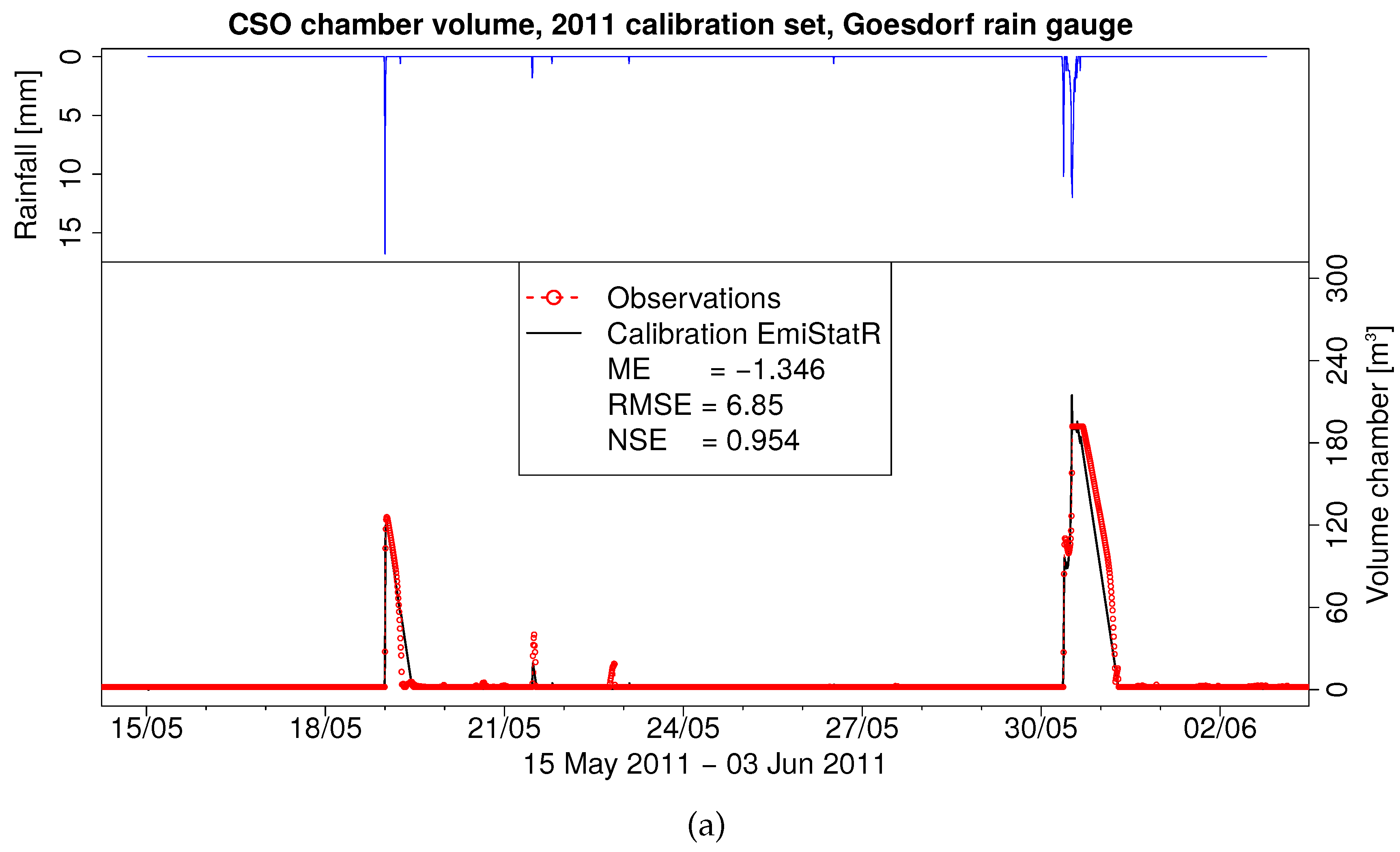
Initial water level, $le{v}_{ini}$	m	[0.1, 3.5]	0.57

and Figure 4a present the final calibration results of the hydraulic model implementing the DREAM algorithm. The calibration required 980 function evaluations. The optimised set of parameters produced a ME of −1.35 m${}^3$, RMSE of 6.85 m${}^3$, and NSE of 0.95. In this case, $Q_{d,max}$ was set to 5 L·s${}^{-1}$ and V was set to 190 m${}^3$ (actual conditions for 2011). Figure 4a shows the precipitation input time series for the calibration dataset (upper inset) and the comparison of observed and simulated time series of the CSOC volume (bottom inset). For the events presented in Figure 4, the values of ME and RMSE are in cubic metres, whereas the NSE is dimensionless. From Figure 4a, it is possible to infer that after model calibration, the model could adequately simulate (NSE = 0.95) the volume in the CSOC. The model simulation was slightly under model observations specifically for low-rainfall conditions. Additionally, an over-prediction of the peak volume was presented in the simulation of the CSOC volume.

3.3. Validation of Model Predictions

Besides the calibration set, another set of measurements was used as independent observations to assess the accuracy of the model predictions for validation of the water quantity model. Input precipitation was recorded from June 3 to July 7, 2011 at a temporal resolution of 1 min, aggregated to 10 min. The observations of water level in the storage CSOC correspond to this period.

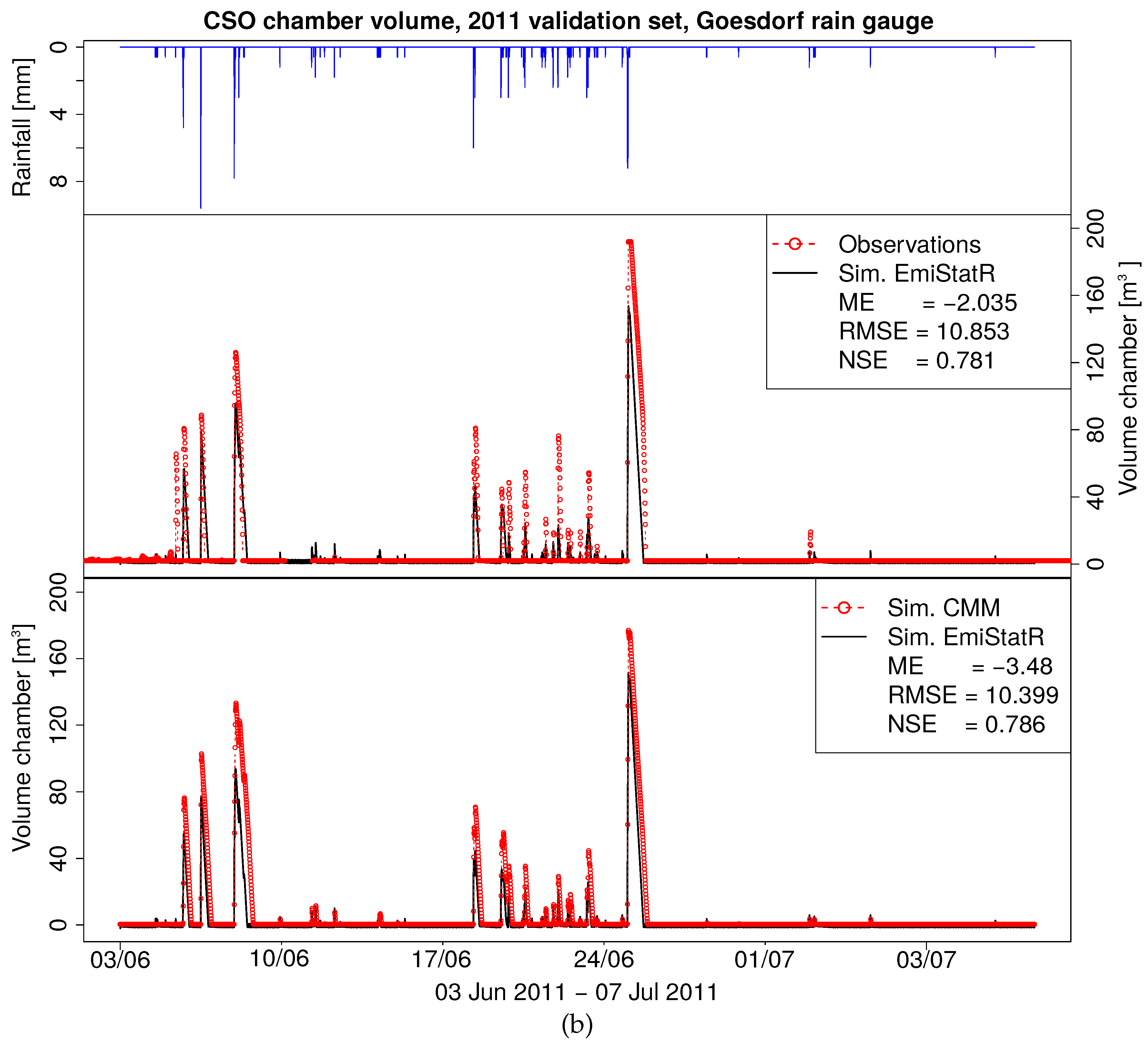
Figure 4b shows the results of the hydraulic model validation. It shows the precipitation input time series (upper inset), the comparison of observed and simulated time series of the CSOC volume (middle inset), and the comparison with the output of a CMM (bottom inset).

The CMM was implemented in the software InfoWorks ICM 7.5 (Innovyze Ltd, Wallingford, Oxfordshire, United Kingdom), and it served as a benchmark to calibrate and validate EmiStatR for water quantity and quality variables. The CMM was a full hydrodynamic flow and pollution load model, which implementd the de Saint Venant partial differential equations and was built initially in the software InfoWorks CS (Innovyze)^® [62]. This model was used to simulate surface run-off and discharge characteristics in local sewer systems and the behaviour of CSO structures in the Goesdorf sub-catchment and future sewer systems linked to weather periods. Besides the catchment data and structural data of sewer sections planned and in operation, the simulations were based on local rain data for local calibration and on regional long-term rain data to simulate the long-term performance of the system. In the framework of a coarse calibration and validation process, it was proved that the model reproduced discharge characteristics in local sewer systems of selected villages sufficiently. The resulting parameterisation to model surface run-off characteristics from impervious areas in the villages, such as initial losses, was applied to further catchments showing similar characteristics [62]. The calibrated model of the catchment and drainage network of the case study, implemented in InfoWorks CS and upgraded to InfoWorks ICM 7.5, was used to validate the performance of EmiStatR. We followed a similar procedure as presented by Meirlaen et al. [28] for developing a mechanistic surrogate model from a CMM.

In general, validation of a good agreement between simulation and observations was observed (NSE of 0.78). The model simulation results were slightly under the observations of the CSOC volume, and as a consequence, the peaks simulated were lower than those of observations, which agreed also with the behaviour shown in Figure 4a.

Regarding the water quality module of EmiStatR, we performed a validation on the basis of a 1 year simulation with the CMM. We ran the validation at 10 min time steps and aggregated the results to 120 min to eliminate short-time variability. Our interest was in the average load of pollutants over several hours, which corresponded well with the usual time for taking water samples for further laboratory analysis. The input values of the two main parameters were 104 $\mathrm{g}·{\mathrm{PE}}^{-1}·{\mathrm{day}}^{-1}$ for $C_{COD,S}$ and 4.7 $\mathrm{g}·{\mathrm{PE}}^{-1}·{\mathrm{day}}^{-1}$ for $C_{NH4,S}$. These values corresponded to wastewater quality (WwQ) measurements. The total COD and NH${}_4$ were monitored in the CSOC under DWF conditions. Figure 4b (bottom inset) shows how the model simulation agreed with observations (NSE of 0.79). The model simulation was also systematically below the observations of CSOC volume.

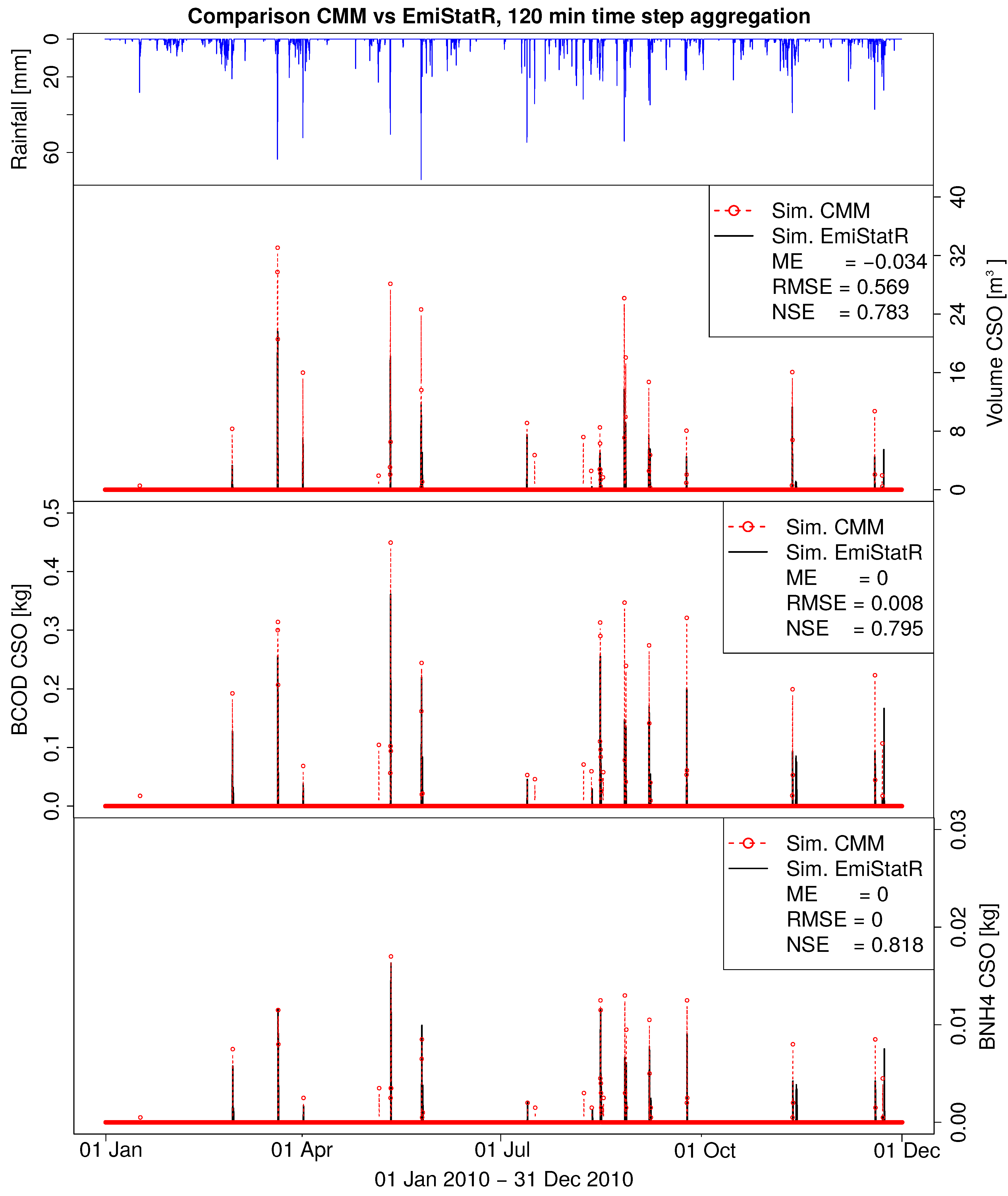
Additionally, to perform a more extensive validation of the water quality model, we compared its output with simulations obtained with the CMM for a 1 year time series at 10 min time steps.

Table 4. Comparison results for the complex mechanistic model (CMM) and EmiStatR (Esch-sur-Sure rain gauge 2 h averages over 1 year period).

Combined Sewer Overflow (CSO) Summary Results	CMM	EmiStatR 1.2.1.0
Period, p (day)	365	365
Duration of CSO spill volume, $d_{Sv}$ (h)	90	100
Frequency of CSO spill volume, $f_{Sv}$ (events)	19	16
Total CSO spill volume, $V_{Sv}$ (m${}^3$)	373	222
Average CSO, $Q_{Sv}$ (L/s)	1.15	0.62
95th percentile of CSO spill volume, $V_{Sv,95}$ (m${}^3$)	27.74	15.26
Maximum CSO spill volume, $V_{Sv,max}$ (m${}^3$)	33.06	21.62
COD total load (BCOD), $B_{COD,Sv}$ (kg)	5.875	4.610
Average BCOD, $B_{COD,Sv,av}$ (kg)	0.131	0.092
95th percentile of BCOD, $B_{COD,Sv,95}$ (kg)	0.320	0.252
Maximum BCOD, $B_{COD,Sv,max}$ (kg)	0.450	0.360
NH${}_4$ total load (BNH4), $B_{NH4,Sv}$ (kg)	0.224	0.208
Average BNH4, $B_{NH4,Sv,av}$ (kg)	0.005	0.004
95th percentile of BNH4, $B_{NH4,Sv,95}$ (kg)	0.012	0.011
Maximum BNH4, $B_{NH4,Sv,95}$ (kg)	0.020	0.020
Run time (min)	30	1.09

and Figure 5 summarise the results of this validation. The results suggest that EmiStatR performed with good accuracy (NSE ≈ 0.80) when compared with the CMM.

3.4. Scalability and Performance

A hardware set-up was defined to execute the scalability test. We used an Intel(R) Xeon(R) CPU E7-L8867 server (Santa Clara, CA, USA) at 2.13 GHz with 40 physical cores (and 40 virtual cores) at 1.064 GHz, 516 GByte in random access memory (RAM), and the operating system (OS) Linux Ubuntu 12.04.5 LTS 64-bit. We used a maximum of $2^5=32$ cores. Additionally, we multiplied the number of simulations by 10 and 100 to evaluate the model runtime under repeated model calls, such as would typically be required in MC uncertainty analyses. As a result, the selected numbers of simulations were 32, 320 and 3200.

Regarding the results of the scalability test, the code implemented in EmiStatR allowed for specifying the number of cores to be used in the simulation according to the number of cores available. In the scalability test, a single simulation referred to a full year at 10 min time steps. We used the calibrated values for Goesdorf. For Kaundorf and Nocher-Route, we used the reference values given in Section 2.3.1.

Table 5. General input data of the EmiStatR scalability test.

General Input	Units	Value
Wastewater
Water consumption, $\mathit{qs}$	$\mathrm{L}·{\mathrm{PE}}^{-1}·{\mathrm{day}}^{-1}$a	150
Daily factors for water consumption,
ATV-A134 curve	–	–
Pollution COD b, $C_{\mathit{COD},S}$	$\mathrm{g}·{\mathrm{PE}}^{-1}·{\mathrm{day}}^{-1}$	120
Pollution NH${}_4$ c, $C_{\mathit{NH}\mathit{4},S}$	$\mathrm{g}·{\mathrm{PE}}^{-1}·{\mathrm{day}}^{-1}$	4.7
Infiltration water
Inflow, $q_f$	L· s${}^{-1}$ · ha${}^{-1}$	0.05
Pollution COD, CODf	$\mathrm{g}·{\mathrm{PE}}^{-1}·{\mathrm{day}}^{-1}$	0
Pollution NH${}_4$, $\mathit{NH}{\mathit{4}}_f$	$\mathrm{g}·{\mathrm{PE}}^{-1}·{\mathrm{day}}^{-1}$	0
Rainwater
Precipitation time series, $P_{\mathit{1}}$	mm	–
Pollution COD, ${\mathit{COD}}_r$	$\mathrm{mg}·{\mathrm{L}}^{-1}$	0
Pollution NH${}_4$, $\mathit{NH}{\mathit{4}}_r$	$\mathrm{mg}·{\mathrm{L}}^{-1}$	0

^a PE: population equivalent; ^b COD: chemical oxygen demand; ^c NH${}_4$: ammonium.

and

Table 6. General input data of the combined sewer overflow (CSO) structures of the EmiStatR scalability test, after calibration for structure 1. Structures 2 and 3 were not calibrated; therefore, reference values were defined.

CSO Input	Sub-Catchment
Identification
ID of the structure	1	2	3
Name of the structure	FBH Goesdorf	FBN Kaundorf	FBH Nocher-Route
Sub-catchment data
Name of the municipality	Goesdorf	Kaundorf	Nocher-Route
Name of the catchment	Haute-Sûre	Haute-Sûre	Haute-Sûre
Number of the catchment	1	1	1
Land use a	R/I	R/I	R/I
Total area, $A_{ges}$ (ha)	30	22	18.6
Impervious area, $A_{imp}$ (ha)	5	11	4.3
Run-off coefficient for impervious area, $C_{imp}$	0.28	0.30	0.30
Run-off coefficient for pervious area, $C_{per}$	0.07	0.10	0.10
Flow time structure, $t_{fS}$ (min)	1	2	2
Population equivalents, $pe$ (PE)	611	358	326
Structure data
Volume, V (m${}^3$)	190	180	157
Curve level–volume, $lev2vol$	Goesdorf	Kaundorf	Nocher-Route
Initial water level, $Le{v}_{ini}$	0.57	1.8	1.8
Maximum throttled outflow, $Q_{d,max}$	5	9	4
Orifice diameter, $D_d$	0.015	0.015	0.015
Orifice coefficient of discharge, $C_d$	0.67	0.67	0.67

summarise the general input data and the CSO structures in the simulation mode, respectively.

Table 7. Runtime in minutes and “speed-up” factor as a function of number of cores used in simulations.

	32 Simulations		320 Simulations		3200 Simulations
Cores	Time	SFa	Time	SF	Time	SF
1	3.4	1.0	33.9	1.0	334.9	1.0
2	1.9	1.8	18.1	1.9	176.6	1.9
4	0.9	3.7	8.9	3.8	87.8	3.8
8	0.6	5.7	4.8	7.0	46.0	7.3
16	0.4	9.1	2.6	13.0	25.3	13.3
32	0.3	12.2	1.5	22.0	14.2	23.6

^a Speed-up factor (SF), computed as the ratio between the time for one core and the time for the ith core.

presents the runtime results in minutes depending on the number of cores used. The row “speed-up” factor (SF) was calculated as the ratio between the maximum computation time and the current computation time. The maximum computation time was set for the computation with just one core, that is, non-parallel computing. The minimum time is presented in bold font for each test. The results indicated speed-up factors of 12.2 (32 MC simulations), 22.0 (320 MC simulations), and 23.6 (3200 MC simulations). The highest speed-up factor (23.6) was obtained in scenario 3 (3200 MC simulations) using 32 cores. Although the lowest computation time was obtained running scenario 1 (32 MC simulations), the lowest speed-up factor was also reached (12.2).

This test was done by setting up the model to simulate three sub-catchments at the same time in parallel mode. Therefore, the scalable code implemented also inferred that parallelisation of sub-catchments also speeds up the overall computation with similar factors.

4. Discussion

4.1. Conceptual and Mathematical Model

EmiStatR is a simplified model. For instance, it does not take the spatial distribution of inputs into account, in particular, rainfall and impervious areas. Additionally, the simulation of the volume and CSO volume, and henceforth pollutant concentrations such as COD and NH${}_4$, as linear combinations of DWF and RWF is a gross simplification of reality. Finally, the model does not take into account additional processes, such as wash-off, first-flush, and hydrodynamics in the sewer network. From the water quality point of view, [4] concludes that, processes typically described by empirical relationships, such as the build-up and wash-off of pollutants, are not very well understood. The simple exponential relationship that is often used is not reliable, and there are few datasets to validate these relationships or to develop new relationships.

The conceptual model EmiStatR was developed for simple catchment models, such as those used for testing purposes. Neither the advection–diffusion nor other solute transport processes for pollutants in the sewer network were implemented, partly because of the fast response of the urban catchments tested. Therefore, comparisons of the EmiStatR framework to other modelling platforms that include solute transport in the sewer networks may be performed. Only one of the urban storm water models analysed by [4] includes the advective–diffusion equation for the transportation of pollutants in pipes, channels, or storages and explains that this equation is not commonly included (1) because of the rapid response of an urban catchment, such that the transport of pollutants by diffusion will be negligible compared with the advection of those pollutants, and (2) because urban storm water infrastructure networks are generally more complex than river networks, and for this reason, the numerical solution of the advective–diffusion equation in complex networks can be computationally expensive.

Harremoës [63] identified important measures in integrated urban drainage modelling: local infiltration, source control, storage basin, local treatment, and real-time control. Thus, the conceptual model implemented in EmiStatR demonstrates the usefulness of local infiltration assessment by considering the variables infiltration flow and water pollution of the infiltration in terms of COD and NH${}_4$. Additionally, the conceptual model implemented serves for testing hypotheses related to the source control by taking into account water consumption and the associated water quality of the wastewater produced in terms of COD and NH${}_4$. Thus, it is possible to take into account the source by means of the evaluation of several profiles for water consumption, as provided by daily profiles, weekly profiles (distinguishing weekend days from weekdays), and seasonal patterns (i.e., monthly patterns accounting for seasonal variability in the source or water consumption). Finally, EmiStatR also takes the storage basin into account by representing the total volume of storage in the catchment as the CSO storage chamber.

EmiStatR is fast and hence very useful for rapid and scalable simulation of long-term scenarios with, for example, yearly precipitation time series as input, as well as for simulating time series with different time-step resolutions from daily to sub-daily time steps. In the case study, we used a time step of 10 min.

4.2. Model Implementation

The implementation of EmiStat in R, as a main advantage, made use of graphical user interfaces (GUIs) and plotting functionalities of R. This implementation saved time in the set-up of the model. The implementation in R was also attractive because EmiStatR can easily be extended with R routines, such as ensuring compatibility of input and output time series with geospatial functionalities implemented in R, for example, through the R package spacetime [64,65]. Moreover, the R environment allows for the implementation of routines for parallel computing and scalable tasks, for example, the packages snowfall [66] and doParallel. The implementation in R was also advantageous because it facilitated the calibration procedures using the DREAM implementation in R.

4.3. Model Calibration and Validation

All simplifications and limitations mentioned above indicate that the model is not perfect and that the model simulations departed from reality. However, despite these simplifications and limitations, the validation results in water quality mode demonstrated a high accuracy. Further uncertainty propagation studies can shed light on how simplifications affect the model output [67]. Such uncertainty propagation evaluations are time-consuming and can best be done with fast and scalable calculators such as EmiStatR.

The plots and validation measures presented in Figure 4 and Figure 5 indicate an accurate representation of the model of the volume in the CSOC at Goesdorf with NSEs of 0.95 for the calibration set, 0.78 for the validation set, and 0.79 when we compared with the CMM. Regarding the simulation of COD and NH${}_4$ loads, Table 4 and Figure 5 show that the model adequately represented the load in the CSO when we compared it with the well-known commercial CMM simulations. This yielded NSEs of 0.80 for the CSO COD load and 0.82 for the CSO NH${}_4$ load.

After comparison of the simulations of EmiStatR with the CMM, the simulation for volume in the CSO was similar (NSE of 0.78), and therefore the loads of COD and NH${}_4$ were represented accurately. Thus we confirmed the hypothesis that for a small catchment system with urban drainage, it is possible to obtain similar accuracy with a surrogate model (in terms of RMSE and NSE) as a CMM.

It is worth noting which physical processes caused the difference between EmiStatR and the CMM. The main difference was that in EmiStatR, we did not model the pipe routing in the sewer system explicitly. This was considered a lumped process and was represented by the $t_{\mathit{fs}}$ factor, which represents the overall travel time in the sewer system until the flow reaches the CSOC. It works well for small case studies, but for large catchments it remains to be seen.

4.4. Scalability

The scalable approach implemented in EmiStatR demonstrated its usefulness and good performance. Computing times decreased substantially, particularly in the scenario with the greatest number of simulations (3200 simulations). The greater the number of simulations, the higher the SF and henceforth the greater the usefulness of the distributed (parallel) computation. This constitutes a promising application of the EmiStatR as a fast calculator in several applications related to urban drainage modelling with increasing levels of complexity and for MC uncertainty analysis.

5. Conclusions

We show using a case study that adequate simulation of CSO spill volume as well as COD and NH${}_4$ loads and concentrations is possible using a scalable, surrogate model. Compared with a CMM, EmiStatR requires less input data, provides automatic calibration procedures, and can present outputs in an accessible way (to practitioners). Another advantage is the large body of R functionalities available to tools such as EmiStatR, for example, compatibility with input and output data formats for temporal and geospatial data and advanced calibration techniques such as DREAM.

We show that EmiStatR provides a satisfactory representation of CSO spill volume and COD and NH${}_4$ loads, which confirms that white box simplification can lead to well-performing surrogate models. Moreover, its inherent parallel computation and scalable capabilities allow fast calculations for scenarios of high complexity and for long-term simulations to test hypotheses in urban drainage modelling.

We compare the results of EmiStatR with those obtained using a well-known CMM. The behaviour for volume in the CSOC and the estimation of loads of COD and NH${}_4$ were very similar. Our case study showed that this small catchment (i.e., area of ≤30 ha) could be modelled with EmiStatR with satisfactory accuracy compared to models of much higher complexity. Future usage will show how EmiStatR performs in other case studies. Because the basis of EmiStatR is formed by generic equations, it is expected that the performance will be similar.

For future work, it would be of interest to the scientific and practitioner communities to take the spatial distribution of some of the input variables, such as precipitation, impervious areas, and land use, into account. The literature shows that spatial variation in precipitation is not considered in many commonly used models [4,16]. Usually, precipitation is assumed to be uniformly distributed in a sub-catchment. This is not a very realistic assumption, particularly in applications for which the response time is short. The integration of geostatistical probability models that interpolate and simulate precipitation data in space and time would be an important advancement in urban drainage modelling.

It should be emphasised that integrated urban drainage modelling often lacks uncertainty propagation tools that assist in quantifying the spatial and temporal (correlated) distributions [68]. It also lack tools for sensitivity analysis to apportion contributions of the different sources of uncertainty to the overall model output uncertainty. Therefore, future work should address these topics and include an economic analysis, also taking the potential failure of CSO infrastructures into account. Such analyses benefit from fast and scalable implementations such as EmiStatR.

References

1. Willems, P. Random number generator or sewer water quality model? Water Sci. Technol. 2006, 54, 387. [Google Scholar] [CrossRef] [PubMed]
2. Beven, K.J. Rainfall-Runoff Modelling: The Primer, 2nd ed.; Wiley-Blackwell: Chichester, West Sussex, UK, 2012. [Google Scholar]
3. United Nations—UN. Transforming Our World: The 2030 Agenda for Sustainable Development; United Nations—UN: New York, NY, USA, 2015. [Google Scholar]
4. Zoppou, C. Review of urban storm water models. Environ. Modell. Softw. 2001, 16, 195–231. [Google Scholar] [CrossRef]
5. Geiger, W.P.; Dorsch, H.R. Quantity–Quality Simulation (QQS): A Detailed Continuous Planning Model for Urban Runoff Control, Volume 1, Model Description, Testing and Applications; US Environmental Protection Agency: Cincinnati, OH, USA, 1980.
6. Huber, W.C.; Dickinson, R.E. Storm Water Management Model, Version 4: User’s Manual; U.S. Environmental Protection Agenc: Athens, GA, USA, 1988. [Google Scholar]
7. Havno, K.; Madsen, M.; Dorge, J. MIKE 11—A generalised river modelling package. In Computer Models of Watershed Hydrology; Singh, V.P., Ed.; Water Resources Publications: Highlands Ranch, CO, USA, 1995; pp. 733–782. [Google Scholar]
8. Mitchell, V.; Duncan, H.; Inman, M.; Rahilly, M.; Stewart, J.; Vieritz, A.; Holt, P.; Grant, A.; Fletcher, T.; Coleman, J.; et al. State of the Art Review of Integrated Urban Water Models; Novatech: Paris, France, 2007; pp. 507–514. [Google Scholar]
9. Mitchell, V.; Mein, R.; McMahon, T. Modelling the Urban Water Cycle. J. Environ. Modell. Softw. 2001, 16, 615–629. [Google Scholar] [CrossRef]
10. Maheepala, S.; Leighton, B.; Mirza, F.; Rahilly, M.; Rahman, J. Hydro Planner—A linked modelling system for water quantity and quality simulation of total water cycle. In MODSIM 2005 International Congress on Modelling and Simulation; Zerger, A., Argent, R.M., Eds.; Modelling and Simulation Society of Australia and New Zealand: Bangkok, Thailand, 2005; pp. 170–176. [Google Scholar]
11. Stewardson, M.; McMahon, T.; Spears, M. Krakatoa: A Model to Assist Integrated Water Resource Management Decision-Making in Urban Areas. In Proceedings of the AWWA 16th Federal Convention, Sydney, Australia, 2–6 April 1995. [Google Scholar]
12. Hardy, M.; Kuczera, G.; Coombes, P. Integrated urban water cycle management: The UrbanCycle model. Water Sci. Tech. 2005, 52, 1–9. [Google Scholar] [CrossRef]
13. DHI, Danish Hydraulic Institute. MIKE URBAN. 2007. Available online: https://www.mikepoweredbydhi.com/products/mike-urban (accessed on 7 June 2018).
14. Mitchell, V.; Diaper, C. UVQ: A tool for assessing the water and contaminant balance impacts of urban development scenarios. Water Sci. Tech. 2005, 52, 91–98. [Google Scholar] [CrossRef]
15. Clark, R.; Pezzaniti, D.; Cresswell, D. Watercress—Community Resource Evaluation and Simulation System—A tool for innovative urban water system planning and design. In Proceedings of the Hydrology and Water Resources Symposium 2002, Melbourne, Australia, 20–23 May 2002. [Google Scholar]
16. Bach, P.M.; Rauch, W.; Mikkelsen, P.S.; McCarthy, D.T.; Deletic, A. A critical review of integrated urban water modelling—Urban drainage and beyond. Environ. Modell. Softw. 2014, 54, 88–107. [Google Scholar] [CrossRef]
17. MWH Soft. InfoWorks CS. Innovyze. 2010. Available online: http://www.innovyze.com/products/infoworks_cs/ (accessed on 7 June 2018).
18. IFAK, Institut für Automation und Kommunikation. SIMBA (Simulation of Biological Wastewater Systems): Manual and Reference; Institut für Automation und Kommunikation e. V: Magdeburg, Germany, 2007. [Google Scholar]
19. Rossman, L. StormWater Management Model—User’s Manual Version 5.0; National Risk Management Research Laboratory, US Environmental Protection Agency: Cincinnati, OH, USA, 2004.
20. Vanhooren, H.; Meirlaen, J.; Amerlinck, Y.; Claeys, F.; Vangheluwe, H.; Vanrolleghem, P. WEST: Modelling biological wastewater treatment. J. Hydroinform. 2003, 5, 27–50. [Google Scholar] [CrossRef]
21. Burger, G.; Fach, S.; Kinzel, H.; Rauch, W. Parallel computing in conceptual sewer simulations. Water Sci. Technol. 2010, 61, 283–291. [Google Scholar] [CrossRef] [PubMed]
22. CRC-CH. MUSIC by eWater. eWater. 2005. Available online: https://ewater.org.au/products/music/ (accessed on 7 June 2018).
23. DHI. MIKE URBAN e Model Manager; DHI: Copenhagen, Denmark, 2009. [Google Scholar]
24. eWater. Urban Developer. 2011. Available online: https://ewater.org.au/products/music/related-tools/urban-developer/ (accessed on 7 June 2018).
25. Rauch, W.; Bach, P.; Brown, R.; Deletic, A.; Ferguson, B.; De Haan, J.; Mccarthy, D.; Kleidorfer, M.; Tapper, N.; Sitzenfrei, R.; et al. Modelling transition in urban drainage management. In Proceedings of the 9th International Conference on Urban Drainage Modelling, Belgrade, Serbia, 4–7 September 2012. [Google Scholar]
26. Rauch, W.; Bertrand-Krajewski, J.L.; Krebs, P.; Mark, O.; Schilling, W.; Schütze, M.; Vanrolleghem, P. Deterministic modelling of integrated urban drainage systems. Water Sci. Technol. 2002, 45, 81–94. [Google Scholar] [CrossRef] [PubMed]
27. Burger, G.; Sitzenfrei, R.; Kleidorfer, M.; Rauch, W. Parallel flow routing in SWMM 5. Environ. Modell. Softw. 2014, 53, 27–34. [Google Scholar] [CrossRef]
28. Meirlaen, J.; Huyghebaert, B.; Sforzi, F.; Benedetti, L.; Vanrolleghem, P. Fast and simultaneous simulation of the integrated urban and wastewater system using mechanistic surrogate models. Water Sci. Technol. 2001, 43, 301–309. [Google Scholar] [CrossRef] [PubMed]
29. Vanrolleghem, P.A.; Benedetti, L.; Meirlaen, J. Modelling and real-time control of the integrated urban wastewater system. Environ. Modell. Softw. 2005, 20, 427–442. [Google Scholar] [CrossRef]
30. Fu, G.; Khu, S.T.; Butler, D. Use of surrogate modelling for multiobjective optimisation of urban wastewater systems. Water Sci. Technol. 2009, 60, 1641–1647. [Google Scholar] [CrossRef] [PubMed] [Green Version]
31. Razavi, S.; Tolson, B.A.; Burn, D.H. Review of surrogate modeling in water resources. Water Resour. Res. 2012, 48, 1–32. [Google Scholar] [CrossRef]
32. Brunetti, G.; Šimunek, J.; Turco, M.; Piro, P. On the use of surrogate-based modeling for the numerical analysis of Low Impact Development techniques. J. Hydrol. 2017, 548, 263–277. [Google Scholar] [CrossRef] [Green Version]
33. Jin, Y. A comprehensive survey of fitness approximation in evolutionary computation. Soft Comput. 2005, 9, 3–12. [Google Scholar] [CrossRef] [Green Version]
34. Meirlaen, J.; Assel, J.V.; Vanrolleghem, P. Real time control of the integrated urban wastewater system using simultaneously simulating surrogate models. Water Sci. Technol. 2002, 45, 109–116. [Google Scholar] [CrossRef] [PubMed]
35. Freni, G.; Maglionico, M.; Mannina, G.; Viviani, G. Comparison between a detailed and a simplified integrated model for the assessment of urban drainage environmental impact on an ephemeral river. Urban Water J. 2008, 5, 87–96. [Google Scholar] [CrossRef]
36. Mannina, G.; Viviani, G. Receiving water quality assessment: Comparison between simplified and detailed integrated urban modelling approaches. Water Sci. Technol. 2010, 62, 2301. [Google Scholar] [CrossRef] [PubMed]
37. Willems, P. Parsimonious Model for Combined Sewer Overflow Pollution. J. Environ. Eng. Am. Soc. Civ. Eng. (ASCE) 2010, 136, 316–325. [Google Scholar] [CrossRef]
38. Coutu, S.; Del Giudice, D.; Rossi, L.; Barry, D.A. Parsimonious hydrological modeling of urban sewer and river catchments. J. Hydrol. 2012, 464–465, 477–484. [Google Scholar] [CrossRef]
39. Vezzaro, L.; Grum, M. A generalised Dynamic Overflow Risk Assessment (DORA) for Real Time Control of urban drainage systems. J. Hydrol. 2014, 515, 292–303. [Google Scholar] [CrossRef] [Green Version]
40. Chen, L.; Ma, Y.; Liu, P.; Xue, W. Parallelisation of a watershed distributed ecohydrological model with dynamic task scheduling. Int. J. Ad Hoc Ubiquitous Comput. 2014, 17, 110–121. [Google Scholar] [CrossRef]
41. Kollet, S.J.; Maxwell, R.M.; Woodward, C.S.; Smith, S.; Vanderborght, J.; Vereecken, H.; Simmer, C. Proof of concept of regional scale hydrologic simulations at hydrologic resolution utilizing massively parallel computer resources. Water Resour. Res. 2010, 46, 1–7. [Google Scholar] [CrossRef]
42. Maxwell, R.M. A terrain-following grid transform and preconditioner for parallel, large-scale, integrated hydrologic modeling. Adv. Water Resour. 2013, 53, 109–117. [Google Scholar] [CrossRef]
43. Claeys, F.; Chtepen, M.; Benedetti, L.; Dhoedt, B.; Vanrolleghem, P.A. Distributed virtual experiments in water quality management. Water Sci. Technol. 2006, 53, 297–305. [Google Scholar] [CrossRef] [PubMed]
44. Burger, G.; Bach, P.M.; Urich, C.; Leonhardt, G.; Kleidorfer, M.; Rauch, W. Designing and implementing a multi-core capable integrated urban drainage modelling Toolkit: Lessons from CityDrain3. Adv. Eng. Softw. 2016, 100, 277–289. [Google Scholar] [CrossRef]
45. Bell, C.D.; Tague, C.L.; McMillan, S.K. A model of hydrology and water quality for stormwater control measures. Environ. Modell. Softw. 2017, 95, 29–47. [Google Scholar] [CrossRef]
46. Sanitary-District. 2015; Welcome to Richmond Indiana. Combined Sewer Overflow. Available online: https://www.richmondindiana.gov/resources/combined-sewer-overflow (accessed on 7 May 2015).
47. R Core Team. R: A Language and Environment for Statistical Computing; R Foundation for Statistical Computing: Vienna, Austria, 2017. [Google Scholar]
48. Vrugt, J.A.; ter Braak, C.J.F.; Diks, C.G.H.; Robinson, B.A.; Hyman, J.M.; Higdon, D. Accelerating Markov chain Monte Carlo simulation by differential evolution with self-adaptive randomized subspace sampling. Int. J. Nonlinear Sci. Numer. Simul. 2009, 10, 273–290. [Google Scholar] [CrossRef]
49. Guillaume, J.; Andrews, F. Dream: DiffeRential Evolution Adaptive Metropolis, R Package version 0.4-2 ed.; Comprehensive R Archive Network (CRAN), 2012. [Google Scholar]
50. Fan, L.; Liu, G.; Wang, F.; Geissen, V.; Ritsema, C.J.; Tong, Y. Water use patterns and conservation in households of Wei River Basin, China. Resour. Conserv. Recyc. 2013, 74, 45–53. [Google Scholar] [CrossRef]
51. DWA. Arbeitsblatt DWA-A 131: Bemessung von Einstufigen Belebungsanlagen; DWA-Regelwerk; DWA: Hennef, Germany, 2002. [Google Scholar]
52. DWA. ATV-DVWK-A 118; DWA-Regelwerk; DWA: Hennef, Germany, 2006. [Google Scholar]
53. Rawls, W.; Long, S.; McCuen, R. Comparison of Urban Flood Frequency Procedures; Paper-American Society of Agricultural Engineers (Microfiche collection): Beltsville, Maryland, 1981.
54. Revolution Analytics; Weston, S. doParallel: Foreach Parallel Adaptor for the “Parallel" Package, R package version 1.0.10; Comprehensive R Archive Network (CRAN), 2015. [Google Scholar]
55. Revolution Analytics; Weston, S. foreach: Provides Foreach Looping Construct for R, R package version 1.4.3; Comprehensive R Archive Network (CRAN), 2015. [Google Scholar]
56. Revolution Analytics; Weston, S. Package “Iterators”: Provides Iterator Construct for R, R package version 1.0.8; Comprehensive R Archive Network (CRAN), 2015. [Google Scholar]
57. Urbanek, S. Multicore: Parallel Processing of R Code on Machines with Multiple Cores or CPUs, R package version 0.1-7; Comprehensive R Archive Network (CRAN), 2013. [Google Scholar]
58. Tierney, L.; Rossini, A.J.; Li, N.; Sevcikova, H. Snow: Simple Network of Workstations, 0.3-13 ed.; R package version 0.4-2; Comprehensive R Archive Network (CRAN), 2016. [Google Scholar]
59. Torres-Matallana, J.; Leopold, U.; Heuvelink, G. stUPscales: An R-package for spatio-temporal Uncertainty Propagation across multiple scales with examples in urban water modelling. Water 2018. under review. [Google Scholar]
60. Ter Braak, C.J.F. A Markov Chain Monte Carlo version of the genetic algorithm Differential Evolution: Easy Bayesian computing for real parameter spaces. Stat. Comput. 2006, 16, 239–249. [Google Scholar] [CrossRef]
61. Nash, J.E.; Sutcliffe, J.E. River flow forecasting through conceptual models. Part 1—A discussion of principles. J. Hydrol. (Amst.) 1970, 10, 282–290. [Google Scholar] [CrossRef]
62. Schutz, G.; Fiorelli, D.; Seiffert, S.; Regneri, M.; Klepiszewski, K. Modelling and Optimal Control of a Sewer Network. In Proceedings of the 9th International Conference on Urban Drainage Modelling, Belgrade, Serbia, 4–7 September 2012. [Google Scholar]
63. Harremoës, P. Integrated urban drainage, status and perspectives. Water Sci. Technol. 2002, 45, 1–10. [Google Scholar] [CrossRef] [PubMed]
64. Pebesma, E. spacetime: Spatio-Temporal Data in R. J. Stat. Softw. 2012, 51, 1–30. [Google Scholar] [CrossRef]
65. Roger, S. Bivand and Edzer Pebesma and Virgilio Gomez-Rubio. In Applied Spatial Data Analysis with R, 2nd ed.; Springer: New York, NY, USA, 2013. [Google Scholar]
66. Knaus, J. Package “Snowfall”: Easier Cluster Computing (Based on Snow), 1.84-6 ed.; The Comprehensive R Archive Network, CRAN, 2015. [Google Scholar]
67. Leon, J.X.; Heuvelink, G.B.M.; Phinn, S.R. Incorporating DEM uncertainty in coastal inundation mapping. PLoS ONE 2014, 9, 1–12. [Google Scholar] [CrossRef] [PubMed]
68. Deletic, A.; Dotto, C.; McCarthy, D.; Kleidorfer, M.; Freni, G.; Mannina, G.; Uhl, M.; Henrichs, M.; Fletcher, T.; Rauch, W.; et al. Assessing uncertainties in urban drainage models. Phys. Chem. Earth 2012, 42-44, 3–10. [Google Scholar] [CrossRef]
Figure 1. Main components of the EmiStatR model: (1) Dry weather flow (DWF) including infiltration flow (IF), (2) pollution of DWF, (3) rain weather flow (RWF), (4) pollution of RWF, (5) combined sewage flow (CSF) and pollution, and (6) combined sewer overflow (CSO) and pollution. CSOC—CSO chamber (background adapted from Sanitary District [46]).
Water 10 00782 g001
Figure 2. Workflow for EmiStatR and the parallelised approach. Parallelisation is set in the input() class, slot(x, “cores”). Level 1: Parallel computing is done inside EmiStatR. Level 2: Parallel computing is done outside of EmiStatR, e.g., Monte Carlo simulation or optimisation.
Water 10 00782 g002
Figure 3. The Haute-Sûre sub-catchment. Combined sewer overflow (CSO) structures are located in Goesdorf (GOE), Kaundorf (KAU), and Nocher-Route (NOR).
Water 10 00782 g003
Figure 4. Rainfall and combined sewer overflow chamber (CSOC) volume at Goesdorf. (a) Time series of May to June 2011 calibrated with DREAM; (b) June to July 2011 simulated time series for validation with observations and the CMM.
Water 10 00782 g004aWater 10 00782 g004b
Figure 5. Rainfall (top), CSO volume (second), chemical oxygen demand (COD) load (third), and NH 4 load (bottom). January to December 2010 time series (Esch-sur-Sûre rain gauge) for validation of EmiStatR using output of a complex mechanistic model (CMM). Simulation at 10 min resolution at Goesdorf; results aggregated to 120 min.
Water 10 00782 g005