stUPscales: An R-Package for Spatio-Temporal Uncertainty Propagation across Multiple Scales with Examples in Urban Water Modelling


Abstract
:
1. Introduction
- (1)
- Lack of tools accounting for reliable uncertainty information of observational and other data.
- (2)
- Lack of tools for reliable information on model structural uncertainty.
- (3)
- Development of tools accounting for spatial, temporal and spatio-temporal uncertainty is still a challenge because many environmental variables are measured at diverse spatial and temporal scales and because there are strong correlations between variables.
- (4)
- Large computational budgets are required when modelling spatio-temporal distributed systems, due to the large number of variables and the correct characterisation of uncertainties and correlations.
- (5)
- Models commonly exhibit complex probability distributions in model output response due to nonlinear responses to model input, even for simple parametric input probability distributions.
- (6)
- The default mechanism to propagate uncertainties is the Monte Carlo method, which is highly computationally demanding. Therefore, large computational resources and implementations of computationally efficient tools are required.
2. Materials and Methods
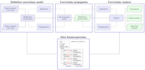
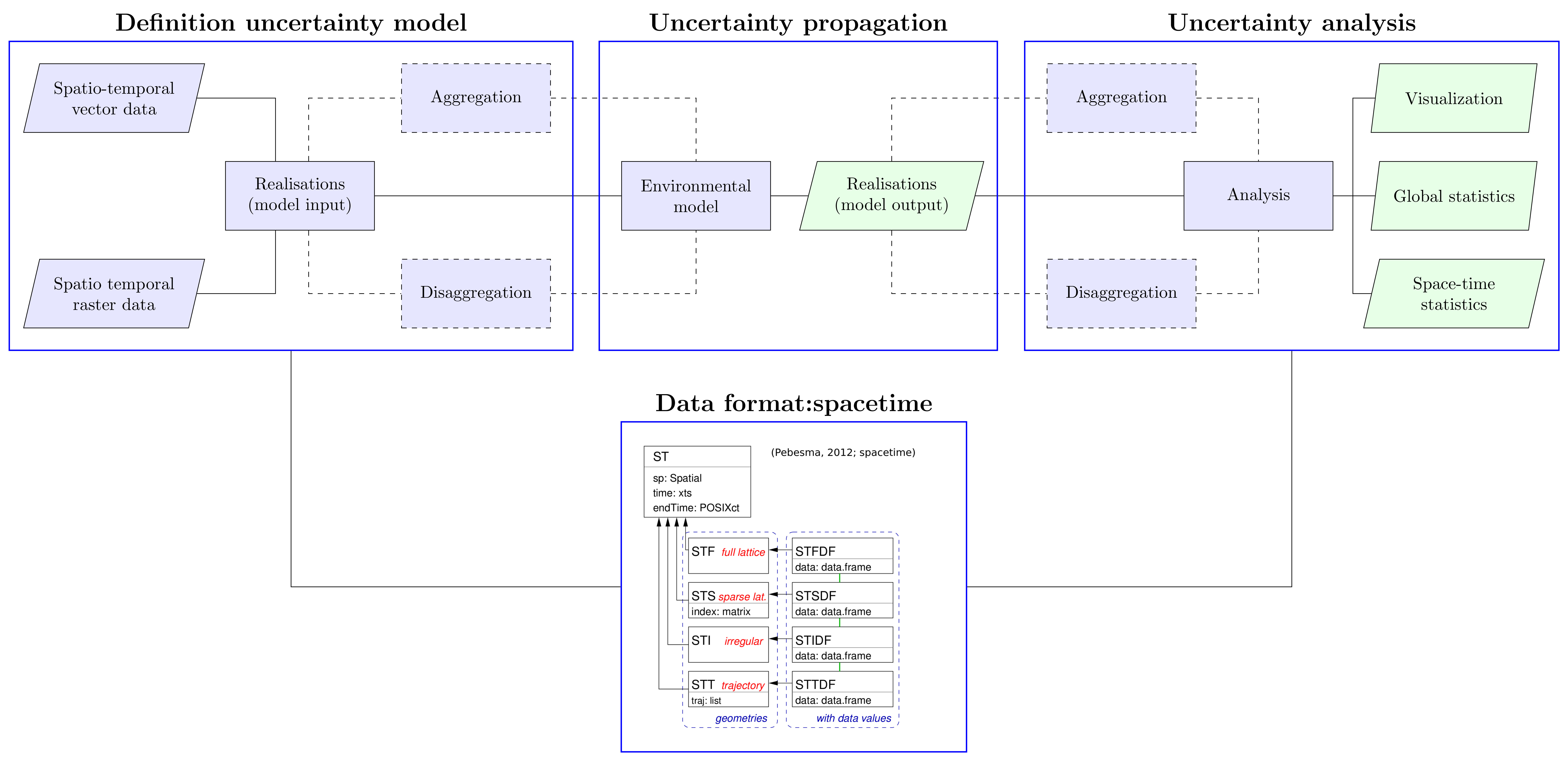
2.1. The R-Package stUPscales
- (1)
- Definition of the uncertainty model (class setup and method MC.setup). Data in raster or vector format are retrieved and the uncertainty model defined. This characterises the input uncertainty in order to generate realisations from the pdfs or, in the case of time series, from uni- or multi-variate autoregressive models;
- (2)
- Uncertainty propagation (method MC.sim). A routine for automation of the chain model input—simulation—model output is defined. This routine is model-dependent and the model input format should match the specific format required by the model. The output format should match the format required by stUpscales. MC simulation is used for propagating model input uncertainty through the environmental model;
- (3)
- Uncertainty analysis (function MC.analysis). Summary statistics such as the mean, variance, and quantiles from the ensemble of MC simulations are computed. In addition, several plots summarising the outcome of the analysis are made.
2.1.1. The Setup Class
- id: Object of class “character” to identify the current MC simulation.
- nsim: Object of class “numeric” to specify the number of MC runs.
- seed: Object of class “numeric” to specify the seed of the random number generator.
- mcCores: Object of class “numeric” to specify the number of cores (CPUs) to be used in the MC simulation.
- st.input: Object of class “character” that defines the name of the file or url of the web service to retrieve the spatio-temporal input data.
- rng: Object of class “list” that contains the names and values of the variables to be used in the MC simulation. Five modes are available: (1) constant value; (2) a variable sampled from a uniform (uni) probability distribution function (pdf); (3) a variable sampled from a normal (nor) pdf; (4) a variable sampled from an autoregressive (AR) model and normal (nor) pdf; (5) a variable sampled from a vector autoregressive (VAR) model and normal (nor) pdf; (6) a variable sampled from discrete values (dis); and (7) a variable sampled from a truncated normal (tnor) pdf.
- ar.model: Object of class “list” containing the coefficients of the AR model as vectors, the name of which is the variable to be modelled and the length of which refers to the order of the model as required by function arima.sim from the base package stats.
- var.model: Object of class “list” containing the vector of intercept terms w, the matrix of AR coefficients A, and the noise covariance matrix C of the VAR model, the name of which is the variable to be modelled and the length of which refers to the order of the model as required by function mAr.sim from the package mAr. For mathematical details, see [27].
2.1.2. The MC.setup Method
2.1.3. The MC.sim Method
- x: Object of class “list” as defined by method MC.setup.
- EmiStatR.cores: a numeric value for specifying the number of cores (CPUs) to be used in the EmiStatR method. Use zero for no use of parallel computation.
2.1.4. The MC.analysis Function
- x: A list from the output of the method MC.sim.
- delta: A numeric value that specifies the level of temporal aggregation required in minutes.
- qUpper: A character string that defines the upper percentile to plot the prediction band of the results. Several options are possible: “q999” the 99.9th percentile, “q995” the 99.5th percentile, “q99” the 99th percentile, “q95” the 95th percentile, and “q50” the 50th percentile. The lower boundary of the prediction band (shown in grey in the output plots) is the 5th percentile in all cases.
- p1.det: A data.frame that contains the time series of the main driving force of the system to be simulated deterministically, e.g., precipitation. This data.frame should have only two columns: the first containing Time [y-m-d h:m:s], the second containing the (numeric) value of the environmental variable.
- sim.det: A list that contains the results of the deterministic simulation, here the output of EmiStatR given p1.det. See the method EmiStatR from the homonym package for details.
- event.ini: A time-date string in POSIXct format that defines the initial time for the event analysis.
- event.end: A time-date string in POSIXct format that defines the final time for the event analysis.
- ntick: A numeric value to specify the number of ticks in the x-axis for the event time-window plots.
- summ: A list provided as MC.analysis output, by default NULL. If provided, the list should contain an output of a previous MC.analysis function, so that the analysis is done again without the calculation of some of the internal variables, thus reducing computation time.
2.1.5. The Agg.t Function
- data: A data.frame that contains the time series of the environmental variable to be aggregated, e.g., precipitation. This data.frame should have two columns: the first is Time [y-m-d h:m:s]; the second the value of the environmental variable. If the environmental variable is different from precipitation, then the column name of the values can be any character string.
- nameData: A character string that defines the name of the environmental variable to be aggregated or an empty string (“ ”).
- delta: A numeric value that specifies the aggregation level required in minutes.
- func: The name of the aggregation function, e.g., mean, sum.
- namePlot: A character string that defines the title of the plot generated.
3. Example 1: Application of stUPscales to Temporal Uncertainty Propagation and Aggregation with the EmiStatR Model
3.1. The Model EmiStatR
3.2. Temporal Aggregation and Model Input Uncertainty Propagation
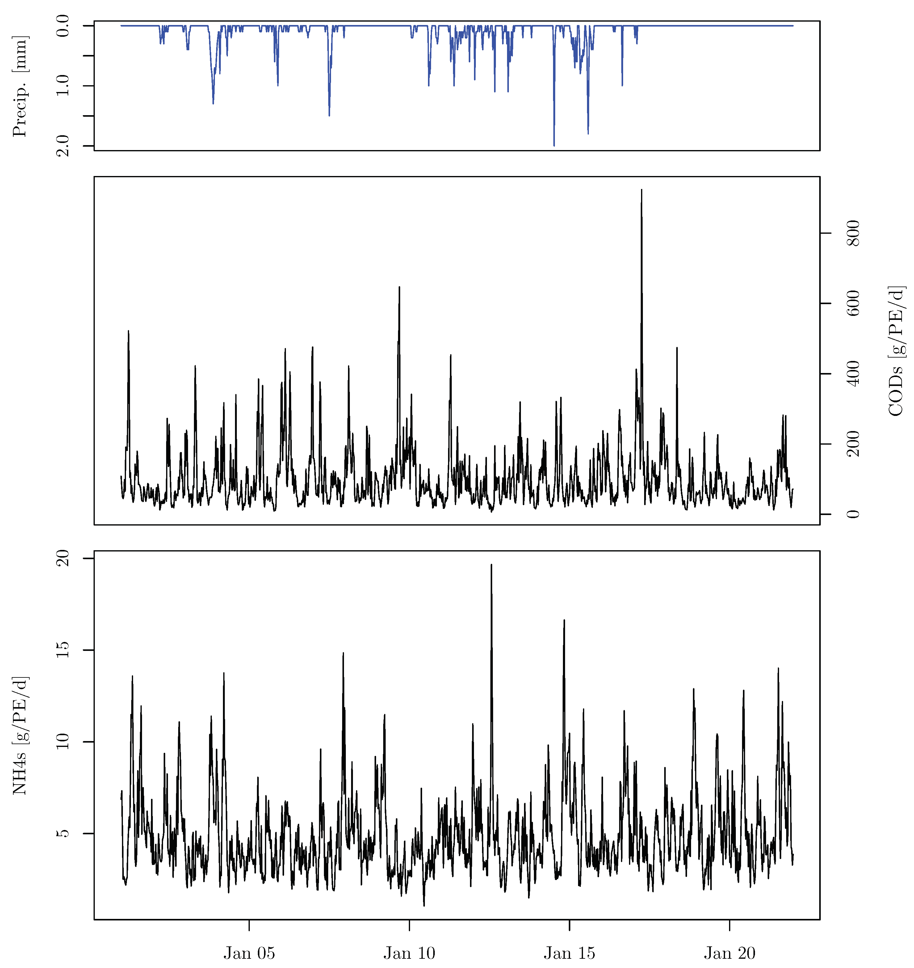
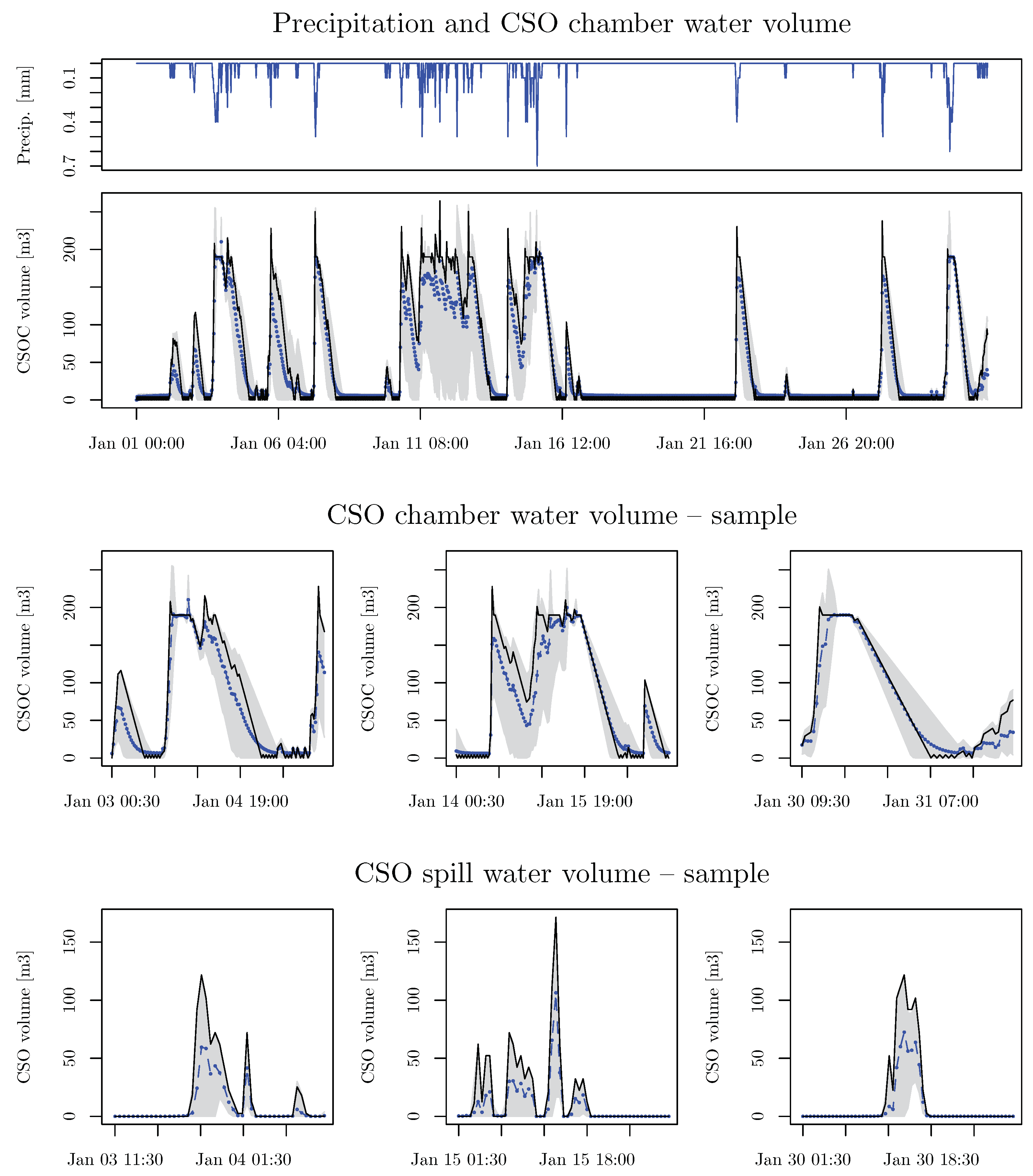
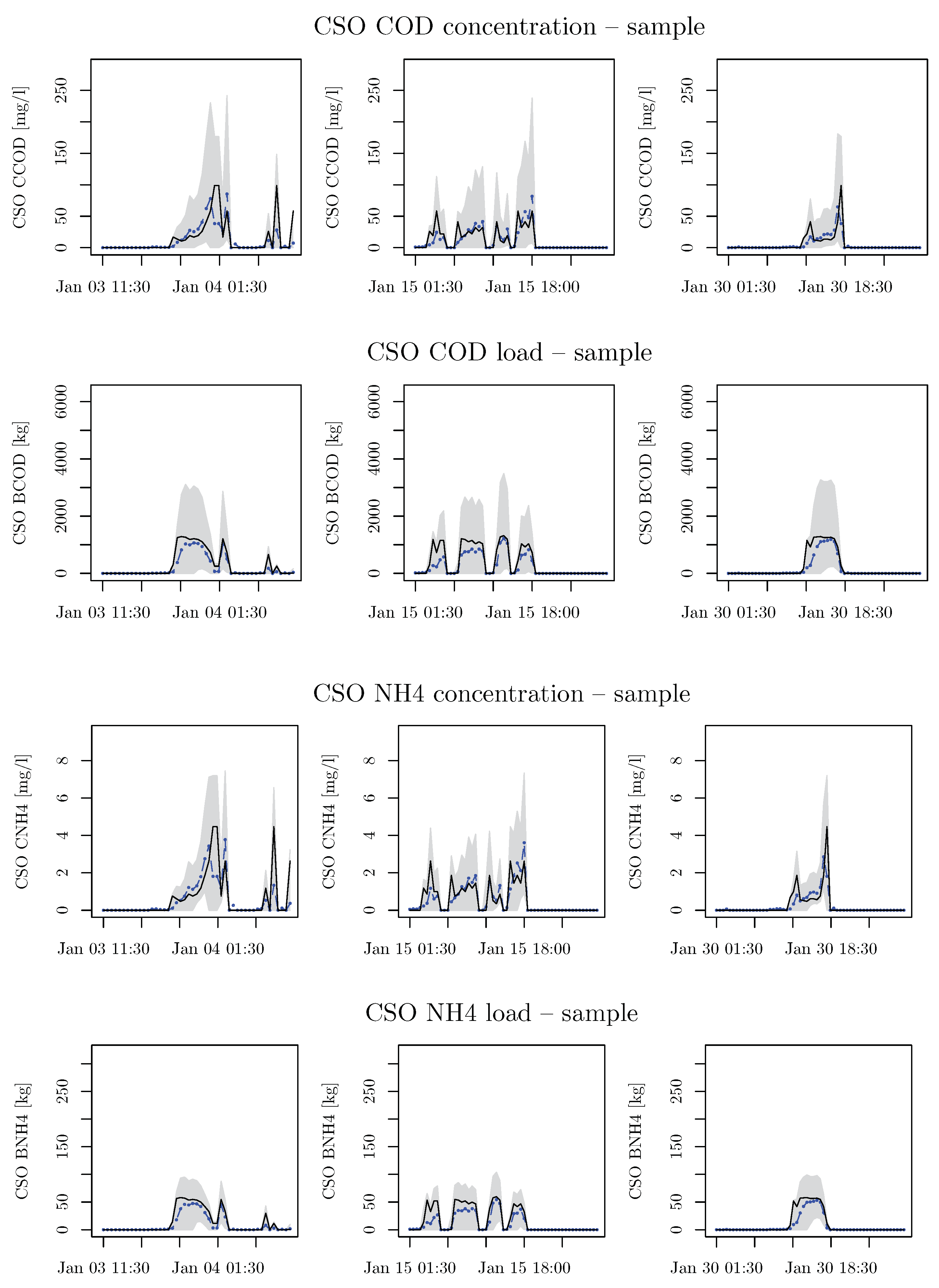
3.3. Results
3.3.1. Model Input
3.3.2. Temporal Aggregation and Model Input Uncertainty Propagation
3.3.3. Model Input Uncertainty and Monte Carlo Simulation Set-Up
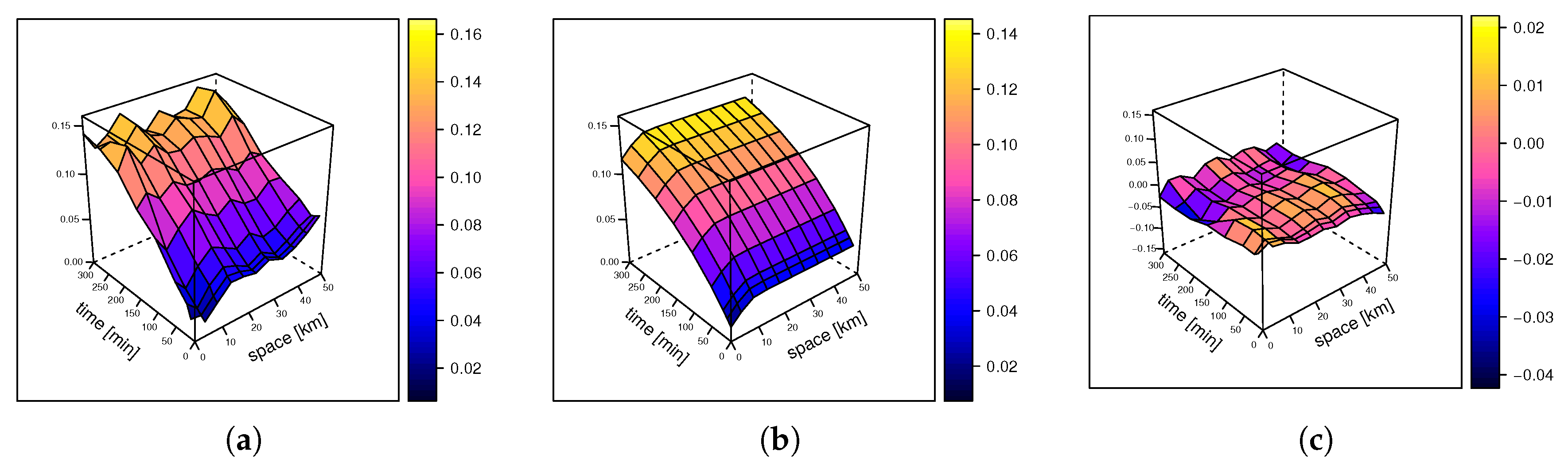
3.3.4. Monte Carlo Simulation and Analysis
4. Example 2: Application of stUPscales to Spatio-Temporal Uncertainty Characterisation of Precipitation for the Grand-Duchy of Luxembourg
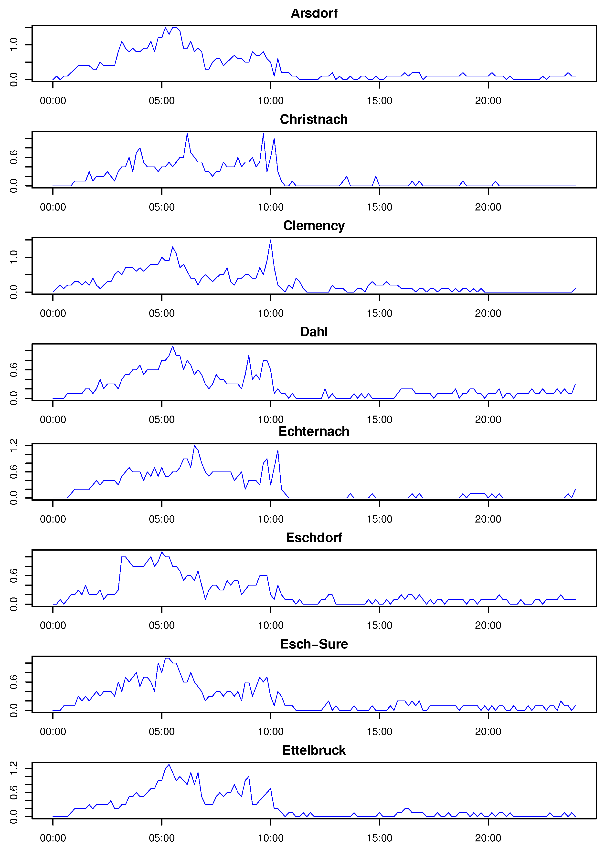
4.1. Selection of Event
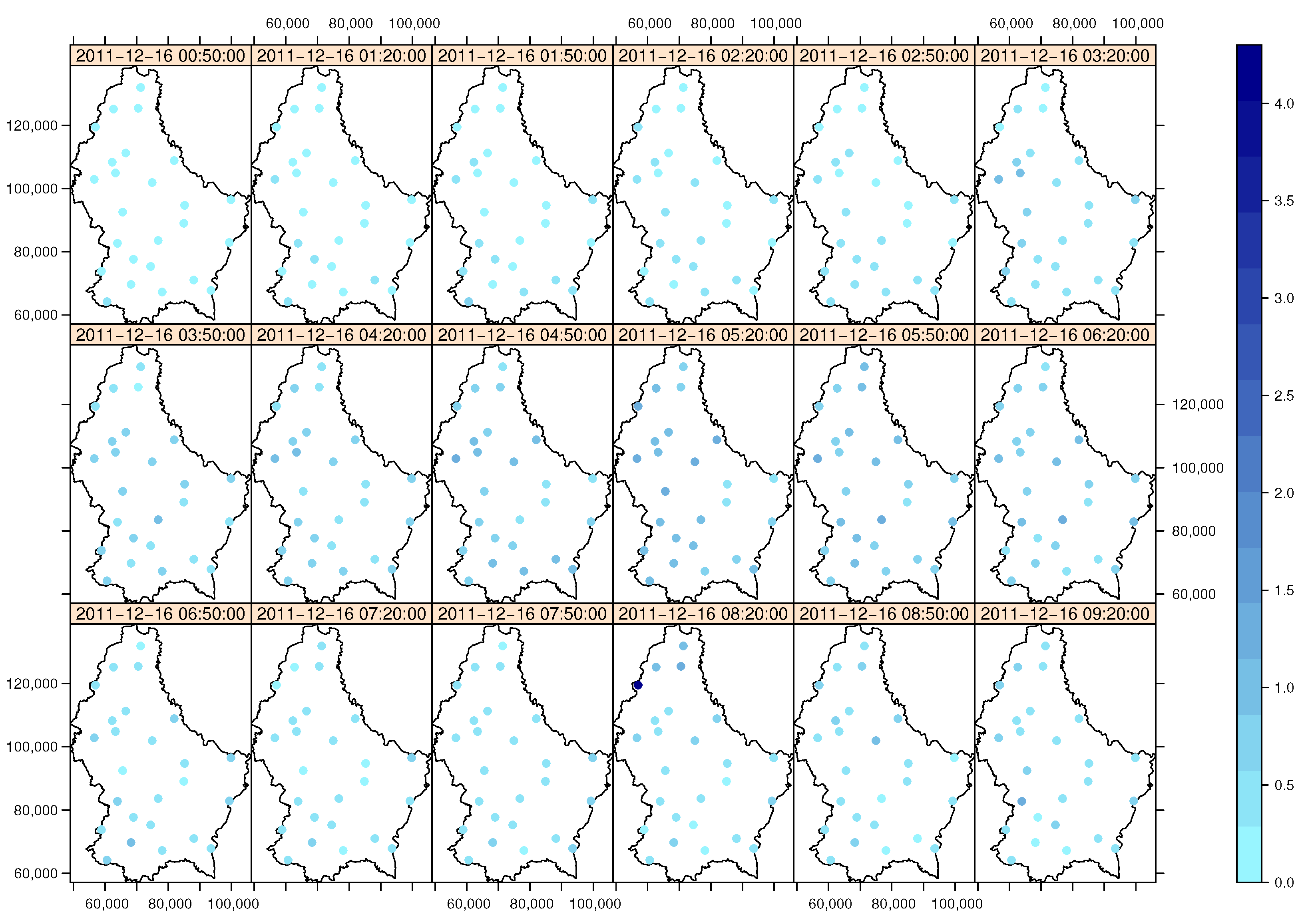
4.2. Ordinary Kriging in the Space-Time Domain
4.3. Results
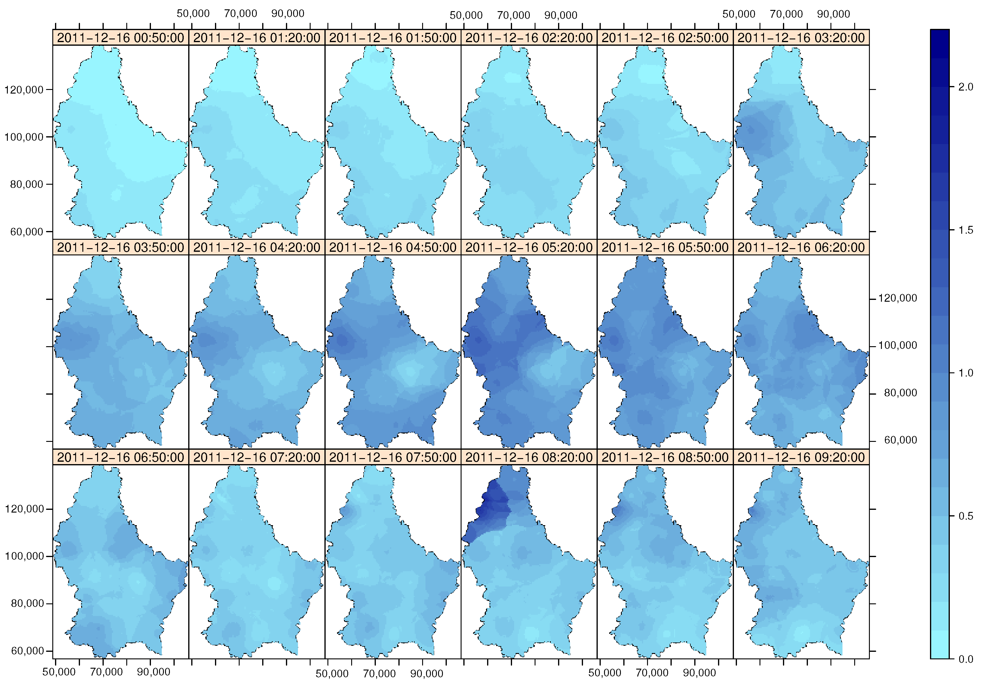
4.3.1. Events Selected and Space-Time Full Grid Object
4.3.2. Space-Time Variograms
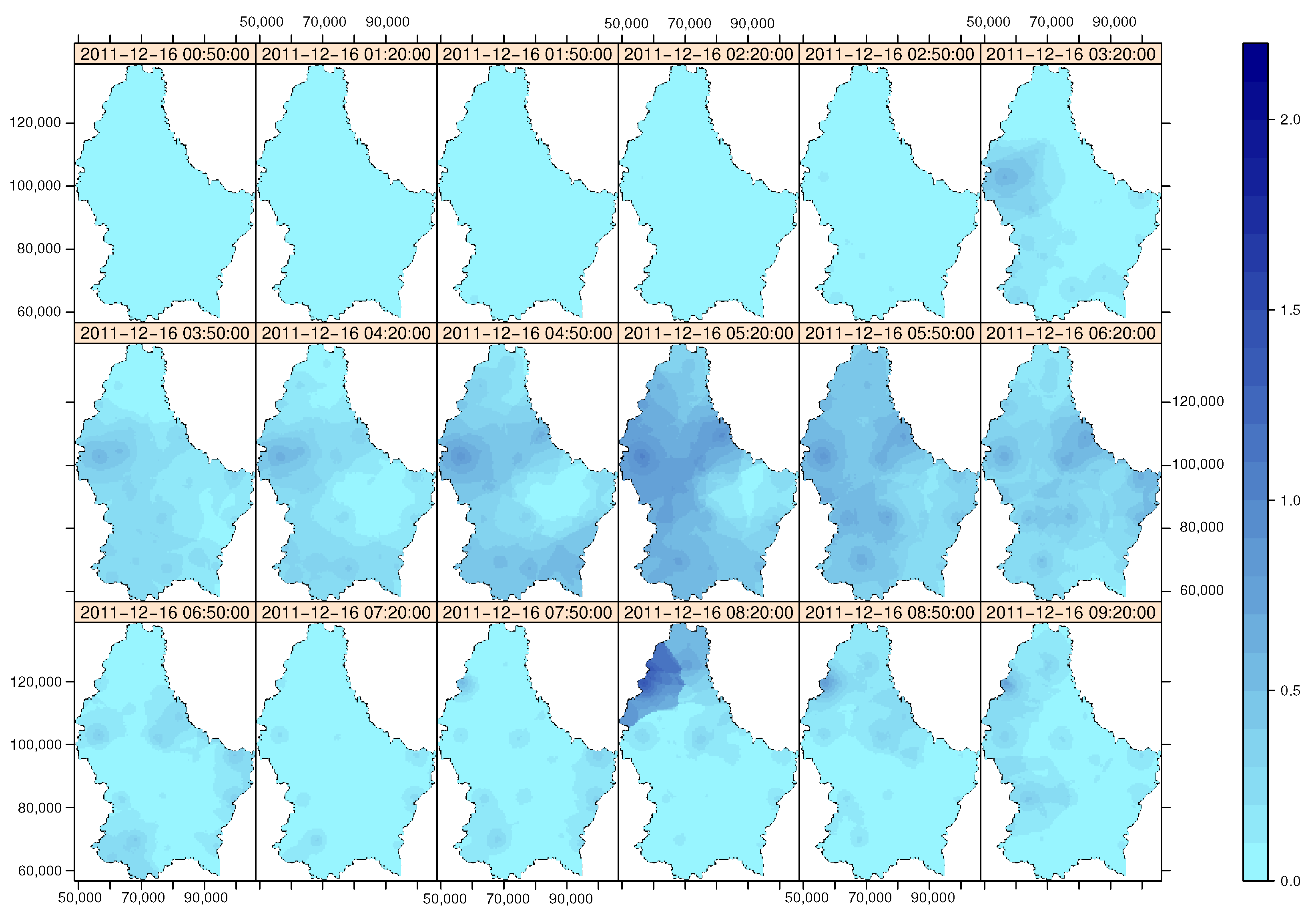
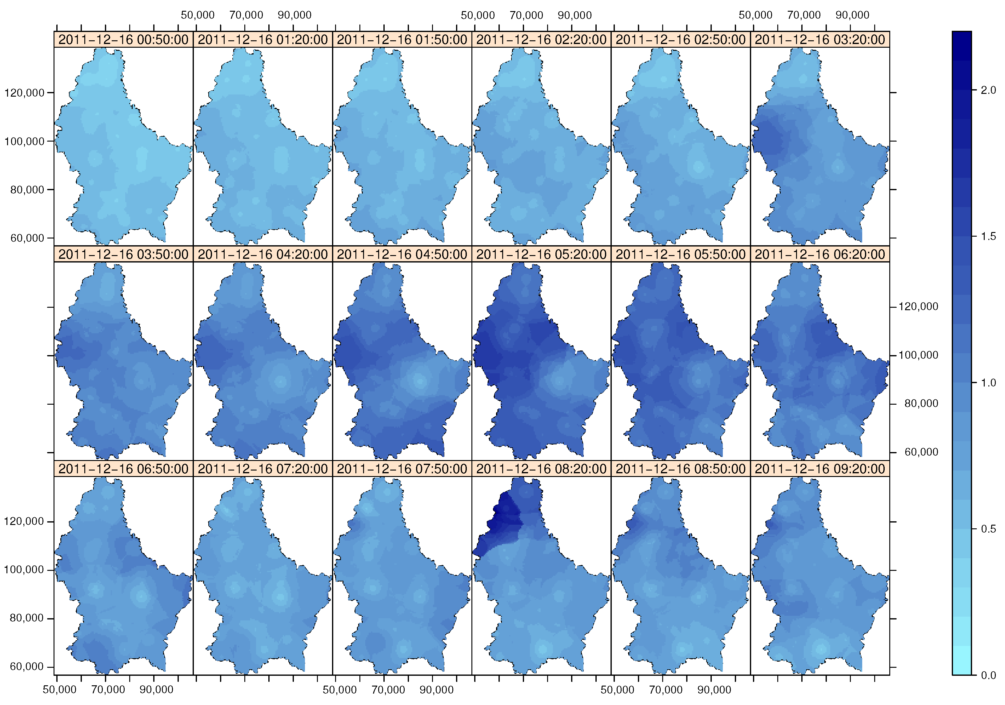
4.3.3. Space-Time Ordinary Kriging
5. Discussion
5.1. Temporal and Spatio-Temporal Model Inputs
5.2. Temporal Aggregation of Model Input
5.3. Model Input Uncertainty Propagation
5.3.1. Model Input Uncertainty and Monte Carlo Simulation Set-Up
5.3.2. Monte Carlo Simulation and Analysis
5.4. Space-Time Characterisation of Model Input Uncertainty
5.5. Data Format for Uncertainties
6. Conclusions and Future Research
Author Contributions
Acknowledgments
Conflicts of Interest
Appendix A
Appendix A.1. The setup Class
> library(stUPscales)
> new_setup <- setup()
> str(new_setup)
Formal class 'setup' [package "stUPscales"] with 8 slots
..@ id : chr "MCsim1"
..@ nsim : num 1
..@ seed : num 0.701
..@ mcCores : num 1
..@ st.input : NULL
..@ rng : NULL
..@ ar.model :List of 1
.. ..$ : NULL
..@ var.model :List of 1
.. ..$ : NULL
Appendix A.2. The MC.setup Method
# case 2: normal autocorrelated time series (AR1 model)
requireNamespace("lmom")
r <- matrix(NA, nrow=nsim, ncol = nrow(st.input))
j <- 1
for(j in 1:nsim){
# r[j,] <- quanor(runif(nrow(st.input)), c(as.numeric(rng[[i]]["mu"]),
as.numeric(rng[[i]]["sigma"])))
y1 <- arima.sim(n = nrow(st.input) , list(order=c(1,0,0),
ar=ar.model[[names(rng)[[i]]]])) # ar =.5
m1 <- mean(y1); s1 <- sd(y1)
m2 <- as.numeric(rng[[i]]["mu"])
s2 <- as.numeric(rng[[i]]["sigma"])
y2 <- m2 +(y1-m1)*s2/s1
r[j,] <- y2
}
par[[i]] <- r
npar <- npar+1
}
# case 5: normal auto- and cross-correlated time series (var.model), parallel code
{
var1 <- (matrix(NA, nrow=1, ncol = nrow(st.input)) )
var2 <- (matrix(NA, nrow=1, ncol = nrow(st.input)) )
obj1 <- 1:nsim
requireNamespace("parallel")
requireNamespace("doParallel")
requireNamespace("foreach")
cl <- makeCluster(mcCores, outfile="")
registerDoParallel(cl, cores=mcCores)
numCores <- detectCores()
rp <- foreach(obj1 = obj1, .packages = c("lmom", "mAr", "parallel", "doParallel",
"foreach"), .export=c("obj1"), .errorhandling = "pass", .verbose=TRUE,
.combine = "rbind") %dopar% {
j <- obj1
print(paste(j, ", ", mcCores, " of ", numCores, " cores for creating
VAR model", sep=""))
y1 <- mAr.sim(w = var.model[["w"]], A = var.model[["A"]],
C = var.model[["C"]], N = nrow(st.input))
# code for only bivariate case
m1 <- mean(y1[,1]); s1 <- sd(y1[,1])
m2 <- as.numeric(rng[[indexVAR[1]]]["mu"])
s2 <- as.numeric(rng[[indexVAR[1]]]["sigma"])
y2 <- m2 +(y1[,1]-m1)*s2/s1
var1[1,] <- y2
m1 <- mean(y1[,2]); s1 <- sd(y1[,2])
m2 <- as.numeric(rng[[indexVAR[2]]]["mu"])
s2 <- as.numeric(rng[[indexVAR[2]]]["sigma"])
y2 <- t(as.data.frame(m2 +(y1[,2]-m1)*s2/s1))
var2[1,] <- y2
return(c(var1, var2))
}
stopCluster(cl)
# closeAllConnections()
# asignation only for bivariate case:
par[[indexVAR[1]]] <- rp[,1:nrow(st.input)]
par[[indexVAR[2]]] <- rp[,(nrow(st.input)+1):(nrow(st.input)*2)]
npar <- npar+2
}
> new_mc_setup <- MC.setup(new_setup)
Appendix A.3. The MC.sim Method
> new_sim <- MC.sim(new_mc_setup)
Appendix A.4. The MC.Analysis Function
> new_analysis <- MC.analysis(new_sim, delta, qUpper, P1.det, sim.det,
+ event.ini, event.end, ntick)
Appendix A.5. The Agg.t Function
> library(stUPscales)
> new_aggregated <- Agg.t(data, nameData, delta, func, namePlot)
Appendix A.6. Example 1: Temporal uNcertainty Propagation and Aggregation
Appendix A.6.1. The Model EmiStatR
> library(EmiStatR)
> new_input <- input()
> str(new_input)
> sim_deterministic <- EmiStatR(new_input)
Appendix A.6.2. Model Input
> library(EmiStatR)
> data("P1")
> summary(P1)
time P [mm]
Min. :2016-01-01 01:00:00 Min. :0.00000
1st Qu.:2016-01-08 18:57:30 1st Qu.:0.00000
Median :2016-01-16 12:55:00 Median :0.00000
Mean :2016-01-16 12:55:00 Mean :0.02007
3rd Qu.:2016-01-24 06:52:30 3rd Qu.:0.00000
Max. :2016-02-01 00:50:00 Max. :0.90000
> sum(P1[,"P [mm]"])
[1] 89.6
Appendix A.6.3. Temporal Aggregation of Model Input
> library(stUPscales)
> P1_30min <- Agg(P1, "P1", 30, sum, "")
> summary(P1_30min)
time Rainfall
Min. :2016-01-01 01:00:00 Min. :0.00000
1st Qu.:2016-01-08 18:52:30 1st Qu. :0.00000
Median :2016-01-16 12:45:00 Median :0.00000
Mean :2016-01-16 12:45:00 Mean :0.06022
3rd Qu.:2016-01-24 06:37:30 3rd Qu. :0.00000
Max. :2016-02-01 00:30:00 Max. :2.00000
> head(P1_30min,3)
time Rainfall
1 2016-01-01 01:00:00 0
2 2016-01-01 01:30:00 0
3 2016-01-01 02:00:00 0
Appendix A.6.4. Model Input Uncertainty and Monte Carlo Simulation Set-Up
> # defining curve level to volume of the storage chamber
> lev2vol <- list(lev = c(.06, 1.10, 1.30, 3.30), vol = c(0, 31, 45, 190))
> new_setup <- setup(id = "MC_1",
+ nsim = 16,
+ seed = 123,
+ mcCores = 8,
+ ts.input = P1_30min,
+ rng = rng <- list(
+ qs = c(pdf = "uni", min = 130, max = 170), # [l/PE/d]
+ CODs = c(pdf = "nor", mu = 4.378, sigma = 0.751), # log[g/PE/d]
+ NH4s = c(pdf = "nor", mu = 1.473, sigma = 0.410), # log[g/PE/d]
+ qf = c(pdf = "uni", min = 0.001, max = 0.1), # [l/s/ha]
+ CODf = 0, # [g/PE/d]
+ NH4f = 0, # [g/PE/d]
+ CODr = 0, # [mg/l]
+ NH4r = 2, # [mg/l]
+ nameCSO = "E1", # [-]
+ id = 1, # [-]
+ ns = "FBH Goesdorf", # [-]
+ nm = "Goesdorf", # [-]
+ nc = "Obersauer", # [-]
+ numc = 1, # [-]
+ use = "R/I", # [-]
+ Atotal = 46, # [ha]
+ Aimp = 25.2, # [ha]
+ Cimp = c(pdf = "uni", min = 0.25, max = 0.95), # [-]
+ Cper = c(pdf = "uni", min = 0.05, max = 0.60), # [-]
+ tfS = 0, # [time steps]
+ pe = c(pdf = "uni", min = 500, max = 800), # [PE]
+ Qd = 6.5, # [l/s]
+ Dd = .150, # [m]
+ Cd = c(pdf = "uni", min = 0.01, max = 2), # [-]
+ V = 190, # [m3] # 1100
+ lev.ini = c(pdf = "uni", min = 0.1, max = 3.5), # [m]
+ lev2vol = lev2vol), # [m] - [m3]
+ ar.model = ar.model <- list(
+ CODs = 0.7, # [-]
+ NH4s = 0.7), # [-]
+ var.model = var.model <- list(inp = c("", "")))
> new_mc_setup <- MC.setup(new_setup)
Appendix A.6.5. Monte Carlo Simulation and Analysis
> new_sim <- MC.sim(newmcsetup, EmiStatR.cores = 0)
> E1 <- list(id = 1, ns = "FBH Goesdorf", nm = "Goesdorf",
+ nc = "Obersauer", numc = 1, use = "R/I",
+ Atotal = 46, Aimp = 25.2, Cimp = 0.86, Cper = 0.55,
+ tfS = -1, pe = 650, Qd = 6.5,
+ Dd = 0.15, Cd = 1.25,
+ V = 190,
+ lev.ini = 0.89,
+ lev2vol = lev2vol)
> input.user <- input(spatial = 0, zero = 1e-5,
+ folder = system.file("shiny", package = "EmiStatR"),
+ cores = 0,
+ ww = list(qs = 150, CODs = 104, NH4s = 4.7),
+ inf = list(qf= 0.05, CODf = 0, NH4f = 0),
+ rw = list(CODr = 0, NH4r = 0, stat = "Dahl"),
+ P1 = P130min, st = list(E1=E1),
+ export = 1)
> sim.det <- EmiStatR(input.user)
> delta <- 30 # minutes
> qUpper <- "q95"
> event.ini <- as.POSIXct("2016-01-12 12:00:00")
> event.end <- as.POSIXct("2016-01-16 05:00:00")
> analysis <- MC.analysis(new_sim, delta, qUpper, P1_30min, sim.det,
+ event.ini, event.end, ntick = 25)
Appendix A.7. Example 2: Spatio-Temporal Uncertainty Characterisation
Appendix A.7.1. Events Selected
> library(stUPscales)
> data("Lux_precipitation")
> summary(event.subset.xts[,1:5])
Index Dahl Echternach
Min. :2011-12-16 00:00:00 Min. :0.0000 Min. :0.000
1st Qu. :2011-12-16 02:30:00 1st Qu. :0.2000 1st Qu. :0.300
Median :2011-12-16 05:00:00 Median :0.4000 Median :0.500
Mean :2011-12-16 05:00:00 Mean :0.4361 Mean :0.482
3rd Qu. :2011-12-16 07:30:00 3rd Qu. :0.6000 3rd Qu. :0.600
Max. :2011-12-16 10:00:00 Max. :1.1000 Max. :1.200
Esch-Sure Eschdorf Ettelbruck
Min. :0.0000 Min. :0.0000 Min. :0.0000
1st Qu. :0.3000 1st Qu.:0.2000 1st Qu.:0.3000
Median :0.4000 Median :0.4000 Median :0.5000
Mean :0.4721 Mean :0.4787 Mean :0.5148
3rd Qu. :0.6000 3rd Qu.:0.8000 3rd Qu.:0.7000
Max. :1.1000 Max. :1.1000 Max. :1.3000
> summary(as.vector(coredata(event.subset.xts)))
Min. 1st Qu. Median Mean 3rd Qu. Max.
0.0000 0.2000 0.4000 0.4616 0.6000 4.3000
Appendix A.7.2. Space-Time Full Grid Object
> data("Lux_stations")
> data("Lux_boundary")
> library(spacetime)
> stfdf <- stConstruct(x = coredata(event.subset.xts),
+ space = list(values=1:ncol(event.subset.xts)),
+ time = index(event.subset.xts),
+ SpatialObj = stations, interval = TRUE)
> library(RColorBrewer)
> sample <- seq.default(from = 6, to = 57, by = 3)
> stplot(stfdf[, sample],
+ col.regions=colorRampPalette(c("cadetblue1","darkblue"))(60),
+ sp.layout = list("sp.polygons", boundary.Lux), scales=list(draw=T),
+ key.space="right", colorkey=T, par.strip.text=list(cex=1),
+ main="Sample from event for prediction",
+ xlim=c(boundary.Lux@bbox[1,]), ylim=c(boundary.Lux@bbox[2,]), cex=1)
Appendix A.7.3. Space-Time Variograms
> library(gstat)
> expVgm <- variogramST(values~1, stfdf, tlags = c(0,1,2,5,10,15,20,25,30),
+ cutoff = 50000, width = 5000)
> linStAni <- estiStAni(expVgm, c(100,50000))
> expVgm$dist <- expVgm$dist/1000
> expVgm$avgDist <- expVgm$avgDist/1000
> expVgm$spacelag <- expVgm$spacelag/1000
> linStAni <- linStAni/1000
> smModel <- vgmST("sumMetric",
+ space = vgm(20, "Sph", 15, 1),
+ time = vgm(10, "Exp", 200, 0),
+ joint = vgm(80, "Sph", 1500, 2.5),
+ stAni = linStAni
+ )
> fitSmModel <- fit.StVariogram(expVgm, smModel, fit.method = 7, stAni=linStAni,
+ method = "L-BFGS-B",
+ lower = c(sill.s = 0, range.s = 0, nugget.s = 0,
+ sill.t = 0, range.t = 0, nugget.t = 0,
+ sill.st= 0, range.st = 10, nugget.st = 0,
+ anis = 40),
+ upper = c(sill.s = 300, range.s = 10, nugget.s = 20,
+ sill.t = 300, range.t = 300, nugget.t = 20,
+ sill.st= 300, range.st = 5E3, nugget.st = 20,
+ anis = 500)
+ )
> attr(fitSmModel, "optim.output")["value"]
\$value
[1] 0.0001309329
> fitSmModel
space component:
model psill range
1 Nug 0.00000000 0
2 Sph 0.02091874 10
time component:
model psill range
1 Nug 0.0000000 0.0000
2 Exp 0.1292266 201.8652
joint component:
model psill range
1 Nug 0.01587417 0.000
2 Sph 0.00000000 1506.002
stAni: 40
Appendix A.7.4. Space-Time Ordinary Kriging
> library(sp)
> grid.scale <- 500
> gridLUX <- SpatialGrid(GridTopology(boundary.Lux@bbox[,1]%/%grid.scale*grid.scale,
+ c(grid.scale,grid.scale),
+ cells.dim=ceiling(apply(boundary.Lux@bbox,1,diff)/grid.scale)))
> proj4string(gridLUX) <- stfdf@sp@proj4string
> fullgrid(gridLUX) <- F
> ind <- over(gridLUX, as(boundary.Lux,"SpatialPolygons"))
> gridLUX <- gridLUX[!is.na(ind)]
> fitSmModel$space$range <- fitSmModel$space$range*1000
> fitSmModel$joint$range <- fitSmModel$joint$range*1000
> fitSmModel$stAni <- fitSmModel$stAni*1000
> LUX_pred <- STF(gridLUX, stfdf@time[sample])
> tIDS <- unique(pmax(1,pmin(as.numeric(outer(-5:5, sample, "+")), nrow(slot(stfdf, "time")))))
> SmPred <- krigeST(values~1, data=stfdf[,tIDS],
+ newdata=LUX_pred, fitSmModel, nmax=50,
+ stAni=fitSmModel[["stAni"]]/10/60,
+ computeVar = T)
> stplot(SmPred, col.regions=colorRampPalette(c("cadetblue1","darkblue"))(60),
+ scales=list(draw=T), main="spatio-temporal sum-metric model",
+ par.strip.text=list(cex=1),
+ sp.layout=list(list(boundary.Lux, fill="transparent")))
> SmPred.var <- SmPred
> SmPred.var[["var1.pred"]] <- SmPred.var[["var1.var"]]
> stplot(SmPred.var, col.regions=colorRampPalette(c("cadetblue1","darkblue"))(60),
+ scales=list(draw=T), main="spatio-temporal sum-metric model (variance)",
+ par.strip.text=list(cex=1),
+ sp.layout=list(list(boundary.Lux, fill="transparent")))
References
- Leopold, U.; Heuvelink, G.B.M.; Tiktak, A.; Finke, P.A.; Schoumans, O. Accounting for change of support in spatial accuracy assessment of modelled soil mineral phosphorous concentration. Geoderma 2006, 130, 368–386. [Google Scholar] [CrossRef]
- Bastin, L.; Cornford, D.; Jones, R.; Heuvelink, G.B.M.; Pebesma, E.; Stasch, C.; Nativi, S.; Mazzetti, P.; Williams, M. Managing uncertainty in integrated environmental modelling: The UncertWeb framework. Environ. Model. Softw. 2013, 39, 116–134. [Google Scholar] [CrossRef] [Green Version]
- Sawicka, K.; Heuvelink, G.B.M.; Walvoort, D. Spatial Uncertainty Propagation Analysis with the spup Package. R J. 2018. under review. [Google Scholar]
- Brown, J.D.; Heuvelink, G.B.M. Assessing Uncertainty Propagation Through Physically based Models of Soil Water Flow and Solute Transport. Encycl. Hydrol. Sci. 2005, 1181–1195. [Google Scholar] [CrossRef]
- Dotto, C.B.S.; Mannina, G.; Kleidorfer, M.; Vezzaro, L.; Henrichs, M.; Mccarthy, D.T.; Freni, G.; Rauch, W.; Deletic, A. Comparison of different uncertainty techniques in urban stormwater quantity and quality modelling. Water Res. 2012, 46, 2545–2558. [Google Scholar] [CrossRef] [PubMed]
- Hengl, T.; Heuvelink, G.B.M.; Van Loon, E.E. On the uncertainty of stream networks derived from elevation data: The error propagation approach. Hydrol. Earth Syst. Sci. 2010, 14, 1153–1165. [Google Scholar] [CrossRef]
- Hamel, P.; Guswa, A.J. Uncertainty analysis of a spatially explicit annual water-balance model: Case study of the Cape Fear basin, North Carolina. Hydrol. Earth Syst. Sci. 2015, 19, 839–853. [Google Scholar] [CrossRef]
- Muthusamy, M.; Schellart, A.; Tait, S.; Heuvelink, G.B.M. Geostatistical upscaling of rain gauge data to support uncertainty analysis of lumped urban hydrological models. Hydrol. Earth Syst. Sci. 2017, 21, 1077–1091. [Google Scholar] [CrossRef]
- Rauch, W.; Bach, P.M.; Brown, R.; Deletic, A.; de Haan, F.; Mair, M.; Kleidorfer, M.; Rogers, B.; Sitzenfrei, R.; Urich, C. Modelling transition in urban water systems. Water Res. 2017, 126, 501–514. [Google Scholar] [CrossRef] [PubMed]
- Nol, L.; Heuvelink, G.B.M.; Veldkamp, A.; de Vries, W.; Kros, J. Uncertainty propagation analysis of an N2O emission model at the plot and landscape scale. Geoderma 2010, 159, 9–23. [Google Scholar] [CrossRef]
- Vanguelova, E.I.; Bonifacio, E.; De Vos, B.; Hoosbeek, M.R.; Berger, T.W.; Vesterdal, L.; Armolaitis, K.; Celi, L.; Dinca, L.; Kjønaas, O.J.; et al. Sources of errors and uncertainties in the assessment of forest soil carbon stocks at different scales—Review and recommendations. Environ. Monit. Assess. 2016, 188, 630. [Google Scholar] [CrossRef] [PubMed]
- Andrianov, G.; Burriel, S.; Cambier, S.; Dutfoy, A.; Dutka-Malen, I.; de Rocquigny, E.; Sudret, B.; Benjamin, P.; Lebrun, R.; Mangeant, F.; et al. Openturns, an open source initiative to treat uncertainties, risks’n statistics in 520 a structured industrial approach. In Proceedings of the ESREL’2007 Safety and Reliability Conference, Stavenger, Norway, 25–27 June 2007. [Google Scholar]
- Adams, B.; Bauman, L.; Bohnhoff, W.; Dalbey, K.; Ebeida, M.; Eddy, J.; Eldred, M.; Hough, P.; Hu, K.; Jakeman, J.; et al. Dakota, a Multilevel Parallel Object-Oriented Framework for Design Optimization, Parameter Estimation, Uncertainty Quantification, and Sensitivity Analysis: Version 5.4 User’S Manual; Report Sandia Technical Report SAND2010-2183; Sandia National Laboratories: Albuquerque, NM, USA, 2009.
- Brown, J.D.; Heuvelink, G.B.M. The data uncertainty engine (due): A software tool for assessing and simulating uncertain environmental variables. Comput. Geosci. 2007, 33, 172–190. [Google Scholar] [CrossRef]
- Schueller, G.I.; Pradlwarter, H.J. Computational stochastic structural analysis (COSSAN)—A software tool. Struct. Saf. 2006, 28, 68–82. [Google Scholar] [CrossRef]
- Pianosia, F.; Sarrazin, F.; Wagener, T. A matlab toolbox for global sensitivity analysis. Environ. Model. Softw. 2015, 70, 80–85. [Google Scholar] [CrossRef]
- Marelli, S.; Sudret, B. UQLab: A Framework for Uncertainty Quantification in Matlab; American Society of Civil Engineers: Reston, VA, USA, 2014; pp. 2554–2563. ISBN 978-0-7844-1360-9. [Google Scholar]
- Kuczera, G.; Parent, E. Monte Carlo assessment of parameter uncertainty in conceptual catchment models: The Metropolis algorithm. J. Hydrol. 1998, 211, 69–85. [Google Scholar] [CrossRef]
- Beven, K.; Binley, A. The future of distributed models: model calibration and uncertainty prediction. Hydrol. Process. 1992, 6, 279–298. [Google Scholar] [CrossRef]
- Vrugt, J.A.; Robinson, B.A. Improved evolutionary optimization from genetically adaptive multimethod search. Proc. Natil. Acad. Sci. USA 2007, 104, 708–711. [Google Scholar] [CrossRef] [PubMed] [Green Version]
- Vrugt, J.A.; Gupta, H.V.; Bouten, W.; Sorooshian, S. A Shuffled Complex Evolution Metropolis algorithm for optimization and uncertainty assessment of hydrologic model parameters. Water Resour. Res. 2003, 39. [Google Scholar] [CrossRef] [Green Version]
- Rauch, W.; Harremoës, P. On the potential of genetic algorithms in urban drainage modeling. Urban Water 1999, 1, 79–89. [Google Scholar] [CrossRef]
- Wijesiri, B.; Egodawatta, P.; McGree, J.; Goonetilleke, A. Assessing uncertainty in pollutant build-up and wash-off processes. Environ. Pollut. 2016, 212, 48–58. [Google Scholar] [CrossRef] [PubMed] [Green Version]
- Ryan, J.A.; Ulrich, J.M. xts: eXtensible Time Series. The Comprehensive R Archive Network, CRAN; R Package Version 0.10-1. 2017. Available online: https://CRAN.R-project.org/package=xts (accessed on 22 June 2018).
- Pebesma, E. Spacetime: Spatio-Temporal Data in R. J. Stat. Softw. 2012, 51, 1–30. [Google Scholar] [CrossRef]
- Hijmans, R.J. Package “Raster”: Geographic Data Analysis and Modeling. The Comprehensive R Archive Network, CRAN. 2014. Available online: https://CRAN.R-project.org/package=raster (accessed on 22 June 2018).
- Luetkepohl, H. New Introduction to Multiple Time Series Analysis; Springer: Berlin, Germany, 2005. [Google Scholar]
- Barbosa, S.M. Package “mAr”: Multivariate AutoRegressive Analysis. The Comprehensive R Archive Network, CRAN. 2015. Available online: https://CRAN.R-project.org/package=mAr (accessed on 22 June 2018).
- Hager, W.H. Wastewater Hydraulics, 2nd ed.; Springer: Berlin, Germany, 2010; p. 652. [Google Scholar]
- Baker, L.A. (Ed.) The Water Environment of Cities; Springer: Berlin, Germany, 2009. [Google Scholar]
- Torres-Matallana, J.A.; Klepiszewski, K.; Leopold, U.; Heuvelink, G.B.M. EmiStatR: A simplified and scalable urban water quality model for simulation of combined sewer overflows. Water 2018, 10, 782. [Google Scholar] [CrossRef]
- Fan, L.; Liu, G.; Wang, F.; Geissen, V.; Ritsema, C.J.; Tong, Y. Water use patterns and conservation in households of Wei River Basin, China. Resour. Conserv. Recycl. 2013, 74, 45–53. [Google Scholar] [CrossRef]
- DWA. Arbeitsblatt DWA-A 131: Bemessung von Einstufigen Belebungsanlagen; DWA-Regelwerk: Hennef, Germany, 2002. [Google Scholar]
- DWA. ATV-DVWK-A 118: Hydraulische Bemessung und Nachweis von Entwässerungssystemen; DWA-Regelwerk: Hennef, Germany, 2006. [Google Scholar]
- Rawls, W.; Long, S.; McCuen, R. Comparison of Urban Flood Frequency Procedures. Preliminary Draft Report Prepared for the Soil Conservation Service; Soil Conservation Service: Beltsville, MD, USA, 1981.
- Gräler, B.; Pebesma, E.; Heuvelink, G.B.M. Spatio-Temporal Interpolation using {gstat}. R J. 2016, 8, 204–218. [Google Scholar]
- Snepvangers, J.J.J.C.; Heuvelink, G.B.M.; Huisman, J.A. Soil water content interpolation using spatio-temporal kriging with external drift. Geoderma 2003, 112, 253–271. [Google Scholar] [CrossRef]
- Bilonick, R.A. Monthly hydrogen ion deposition maps for the northeastern U.S. from July 1982 to September 1984. Atmos. Environ. 1988, 22, 1909–1924. [Google Scholar] [CrossRef]
- Pebesma, E.J. Multivariable geostatistics in S: The “gstat” package. Comput. Geosci. 2004, 30, 683–691. [Google Scholar] [CrossRef]
- Pebesma, E.; Bivand, R. Package “sp”: Classes and Methods for Spatial Data. The Comprehensive R Archive Network, CRAN. 2005. Available online: https://CRAN.R-project.org/package=sp (accessed on 22 June 2018).
- Byrd, R.H.; Lu, P.; Nocedal, J.; Zhu, C. A Limited Memory Algorithm for Bound Constrained Optimization. SIAM J. Sci. Comput. 1995, 16, 1190–1208. [Google Scholar] [CrossRef] [Green Version]
- Moret, S.; Codina Gironès, V.; Bierlaire, M.; Maréchal, F. Characterization of input uncertainties in strategic energy planning models. Appl. Energy 2017, 202, 597–617. [Google Scholar] [CrossRef]
- Tock, L.; Maréchal, F. Decision support for ranking Pareto optimal process designs under uncertain market conditions. Comput. Chem. Eng. 2015, 83, 165–175. [Google Scholar] [CrossRef] [Green Version]
- Dubuis, M. Energy System Design Under Uncertainty. Ph.D. Thesis, École Polytechnique Fédérale De Lausanne, Lausanne, Switzerland, 2012. [Google Scholar]
- Pye, S.; Sabio, N.; Strachan, N. An integrated systematic analysis of uncertainties in UK energy transition pathways. Energy Policy 2015, 87, 673–684. [Google Scholar] [CrossRef]
- Sin, G.; Gernaey, K.V.; Neumann, M.B.; van Loosdrecht, M.C.M.; Gujer, W. Uncertainty analysis in WWTP model applications: A critical discussion using an example from design. Water Res. 2009, 43, 2894–2906. [Google Scholar] [CrossRef] [PubMed]
- Lythcke-Jørgensen, C.; Ensinas, A.V.; Münster, M.; Haglind, F. A methodology for designing flexible multi-generation systems. Energy 2016, 110, 34–54. [Google Scholar] [CrossRef] [Green Version]
- Zoppou, C. Review of urban storm water models. Environ. Model. Softw. 2001, 16, 195–231. [Google Scholar] [CrossRef]
- Bertsimas, D.; Sim, M. The Price of Robustness. Oper. Res. 2004, 52, 35–53. [Google Scholar] [CrossRef]
- Pebesma, E. Package gstat: Spatial and Spatio-Temporal Geostatistical Modelling, Prediction and Simulation. The Comprehensive R Archive Network, CRAN. 2012. Available online: https://CRAN.R-project.org/package=gstat (accessed on 22 June 2018).
- Williams, M.; Cornford, D.; Bastin, L.; Pebesma, E. Uncertainty Markup Language (UnCertML); Technical Report; The Open Geospatial Consortium Inc.: Wayland, MA, USA, 2009. [Google Scholar]


| General Input | Units | CSO Input | Units |
|---|---|---|---|
| Wastewater | Catchment data | ||
| Water consumption, | a | Total area, | [ha] |
| Pollution COD b, | Impervious area, | [ha] | |
| Pollution NH c, | Run-off coefficient for impervious area, | [-] | |
| Run-off coefficient for pervious area, | [-] | ||
| Infiltration water | Theoretical largest flow time structure, | [time step] | |
| Inflow, | [L · s · ha] | Population equivalents, | [PE] |
| Pollution COD, | |||
| Pollution NH, | CSO structure data | ||
| Volume, V | [m] | ||
| Rainwater | Curve level—volume, | [m], [m] | |
| Precipitation time series, P | [mm] | Initial water level, | [m] |
| Pollution COD, | Maximum throttled outflow, | [L · s] | |
| Pollution NH, | Orifice diameter, | [m] | |
| Orifice coefficient of discharge, | [-] |
| Variable | Unit | |
|---|---|---|
| CSO a summary | Period, p | [day] |
| Total CSO chamber volume, | [m] | |
| Duration CSO spill volume, | [h] | |
| Frequency CSO spill volume, | [events] | |
| Total CSO spill volume, | [m] | |
| Average CSO flow, | [L/s] | |
| 95th percentile CSO spill volume, | [m] | |
| Maximum CSO spill volume, | [m] | |
| COD b in spill volume | Total CCOD c, | [mg/L] |
| Average CCOD, | [mg/L] | |
| 95th percentile CCOD, | [mg/L] | |
| Maximum CCOD, | [mg/L] | |
| Total BCOD d, | [kg] | |
| Average BCOD, | [kg] | |
| 95th percentile BCOD, | [kg] | |
| Maximum BCOD, | [kg] | |
| NH e in spill volume | Total CNH4, | [mg/L] |
| Average CNH4 f, | [mg/L] | |
| 95th percentile CNH4, | [mg/L] | |
| Maximum CNH4, | [mg/L] | |
| Total BNH4 g, | [kg] | |
| Average BNH4, | [kg] | |
| 95th percentile BNH4, | [kg] | |
| Maximum BNH4, | [kg] |
| Input | Units | Reference | Literature | Range |
|---|---|---|---|---|
| Value | Source | (This Study) | ||
| Wastewater | ||||
| Water consumption, | a | 150 b | [32] | [130, 170] |
| Pollution COD c, | 120 | [33] | [90, 150] | |
| Pollution TKN d | 11 | [33] | [7, 15] | |
| Pollution NH e | 4.7 | [31] | [1, 8] | |
| Infiltration water | ||||
| Inflow, | [L · s · ha] | 0.05 | [34] | [0.001, 0.1] |
| Catchment data | ||||
| Run-off coefficient for impervious area, | [-] | See [35] | [35] | [0.20, 0.95] |
| Run-off coefficient for pervious area, | [-] | See [35] | [35] | [0.05, 0.50] |
| Flow time structure, | [time step] | 2 | [31] | [0, 12] |
| CSO structure data | ||||
| Initial water level, | [m] | f/2 | [31] | [0, ] |
| Orifice coefficient of discharge, | [-] | 1.25 | [31] | [0.01, 2] |
| Partial Sill | Range | |
|---|---|---|
| Spatial component | ||
| Nugget | 0 | 0 |
| Spherical | 0.021 | 10 |
| Time component | ||
| Nugget | 0 | 0 |
| Exponential | 0.129 | 201.9 |
| Joint component | ||
| Nugget | 0.016 | 0 |
© 2018 by the authors. Licensee MDPI, Basel, Switzerland. This article is an open access article distributed under the terms and conditions of the Creative Commons Attribution (CC BY) license (http://creativecommons.org/licenses/by/4.0/).
Share and Cite
Torres-Matallana, J.A.; Leopold, U.; Heuvelink, G.B.M. stUPscales: An R-Package for Spatio-Temporal Uncertainty Propagation across Multiple Scales with Examples in Urban Water Modelling. Water 2018, 10, 837. https://doi.org/10.3390/w10070837
Torres-Matallana JA, Leopold U, Heuvelink GBM. stUPscales: An R-Package for Spatio-Temporal Uncertainty Propagation across Multiple Scales with Examples in Urban Water Modelling. Water. 2018; 10(7):837. https://doi.org/10.3390/w10070837
Chicago/Turabian StyleTorres-Matallana, Jairo Arturo, Ulrich Leopold, and Gerard B. M. Heuvelink. 2018. "stUPscales: An R-Package for Spatio-Temporal Uncertainty Propagation across Multiple Scales with Examples in Urban Water Modelling" Water 10, no. 7: 837. https://doi.org/10.3390/w10070837