
High-Frequency Observations of Cyanobacterial Blooms in Lake Taihu (China) from FY-4B/AGRI
by
Xin Hang
1,
Xinyi Li
2,
Yachun Li
1,*,
Shihua Zhu
1,
Shengqi Li
3,
Xiuzhen Han
4,* and
Liangxiao Sun
1 1
Jiangsu Climate Center, Jiangsu Meteorological Bureau, Nanjing 210008, China
2
Nanjing Joint Institute for Atmospheric Sciences, Nanjing 210009, China
3
School of Atmospheric Physics, Nanjing University of Information Science and Technology, Nanjing 210044, China
4
National Satellite Meteorological Center, Beijing 100081, China
*
Authors to whom correspondence should be addressed.
Water 2023, 15(12), 2165; https://doi.org/10.3390/w15122165
Submission received: 21 February 2023
/
Revised: 3 June 2023
/
Accepted: 6 June 2023
/
Published: 8 June 2023
(This article belongs to the Special Issue Remote Sensing-Based Study on Surface Water Environment)
Abstract
:China’s FY-4B satellite, launched on 3 June 2021, is a new-generation geostationary meteorological satellite. The Advanced Geosynchronous Radiation Imager (AGRI) onboard FY-4B has 15 spectral channels, including 2 visible (470 and 650 nm), 1 near infrared (825 nm), and 3 shortwave infrared (1379, 1610, and 2225 nm) bands, which can be used to observe the Earth system with the highest spatial resolution of 500 m and 15 min temporal resolution. In this study, FY-4B/AGRI observations were applied for the first time to monitor cyanobacterial blooms in Lake Taihu, China. The AGRI reflectance at visible and near-infrared bands was first corrected to surface reflectance using the 6S radiative transfer model. Due to the similar spectral reflectance characteristics to those of land-based vegetation, the normalized difference vegetation index (NDVI) and some other remote sensing vegetation indices are usually used for the retrieval of cyanobacterial blooms. The fractional vegetation cover (FVC) of algae, defined as the fraction of green vegetation in the nadir view, was adopted to depict the status and trend of cyanobacterial blooms. NDVI and FVC, the two remote sensing indices developed for the retrieval of land vegetation, were used for the detection of cyanobacteria blooms in Lake Taihu. Finally, the FVC derived from AGRI measurements was compared with that obtained from the Advanced Himawari Imager (AHI) onboard the Himawari-8 satellite to validate the effectiveness of our method. It was found that atmospheric correction can substantially improve the determination of the normalized difference vegetation index (NDVI) values of cyanobacterial blooms in the lake. As a proof of the robustness of the algorithm, the NDVIs are both derived from both AGRI and AHI and their magnitudes are similar. In addition, the distribution of cyanobacterial blooms derived from AGRI FVC is highly consistent with that derived from FY-3D/MERSI and EOS/MODIS. While a lower spatial resolution of FY-4B/AGRI might restrict its capability in capturing some spatial details of cyanobacterial blooms, the high-frequency measurements can provide information for the timely and effective management of aquatic ecosystems and help researchers better quantify and understand the dynamics of cyanobacterial blooms. In particular, AGRI can provide greater details on the diurnal variation in the distribution of cyanobacterial blooms owing to the high temporal resolution.
1. Introduction
In recent decades, most inland lakes globally have faced increasing problems associated with water eutrophication owing to high-intensity human activities. One of the most serious consequences of eutrophication is the globally increasing frequency of cyanobacterial blooms in inland waters [1,2], and some other evidence suggests that co-occurring microorganisms also play an important role in the occurrence of cyanobacteria blooms under non-eutrophication conditions [3,4]. Some evidence shows that cyanobacterial blooms occur in 30–40% of lakes and reservoirs in the world and, more seriously, in up to approximately 80% of inland freshwater bodies in developing countries such as China [5]. Some species of cyanobacteria can form toxic blooms in freshwater and marine environments that can threaten ecosystem function and degrade water quality, affecting recreation, drinking water supplies, fisheries, the co-occurring microorganism’s assembly and community succession, and human health [3,4,5,6]. Moreover, climate change has further intensified the frequency of occurrence of cyanobacterial blooms and enhanced the associated hazards [7,8,9]. For example, with climate warming and rising CO2 levels, the competitive advantage of cyanobacteria significantly increases, which facilitates their proliferation in eutrophic lakes. The increase in variability of precipitation and the possibility of heavy precipitation will exacerbate the loss of nutrients such as nitrogen and phosphorus in the soil, leading to an increase in the concentration of nutrients in lakes. However, the existing tools have limited monitoring capabilities for cyanobacterial blooms. Consequently, new tools and technologies are needed for the rapid detection, characterization, and mitigation of cyanobacterial blooms that can threaten water security.
Developments in satellite remote sensing technology mean that the resolution and acquisition of parameter information and the observation accuracy of remotely sensed data and images have improved substantially. Due to the large spatial coverage and short revisit interval of some satellite sensors, optical remote sensing could be used to effectively and efficiently monitor cyanobacteria blooms [10,11]. Recent studies have also demonstrated the potential of remote sensing-based technology for estimating chlorophyll-a concentration in eutrophic lakes worldwide [12,13,14]. Remote sensing can provide valuable information about the density, scope, and potential impact of cyanobacterial blooms owing to its advantages of a wide monitoring range, fast speed, and ease of long-term dynamic monitoring [15,16]. Owing to their high spatial and spectral resolutions, the Medium-Resolution Spectral Imager (MERSI), Moderate-Resolution Imaging Spectroradiometer (MODIS), and Landsat have all been used for detecting cyanobacterial blooms in inland lakes [9,17]. However, these sensors cannot provide optimum observation frequency, e.g., the MODIS sensors onboard the Terra and Aqua satellites can provide at most one observation daily (usually at around solar noon), and effective data cannot be obtained during cloudy weather. Therefore, more high-frequency observations are needed to improve the acquisition of information on highly dynamic aquatic environments under varying weather conditions, which could play a key role in developing early warning, early prevention, and early disposal strategies to control cyanobacterial blooms and ensure the safety of urban drinking water. Cyanobacteria dynamics represent an important scientific topic, and previous related studies have confirmed that it is difficult to objectively reveal long-term cyanobacteria dynamics using only satellite data with low temporal resolution [18]. High-frequency satellite observations would minimize the amount of missing information due to cloud cover, which could ensure a more accurate evaluation of cyanobacterial bloom events, help improve understanding of cyanobacteria dynamics, and reduce the uncertainty of estimations of carbon fixation associated with cyanobacterial blooms [19].
Although polar-orbiting satellite data have been used extensively for monitoring the aquatic environment of inland lakes, the advantages of geostationary satellites have not been explored fully in relation to retrievals of cyanobacterial blooms. China’s new geostationary meteorological satellite FY-4B was launched in June 2021 and is now operated by the China Meteorological Administration. The Advanced Geosynchronous Radiation Imager (AGRI) onboard FY-4B has 15 spectral channels, 6 of which are in the range of visible (VIS) to shortwave infrared (SWIR) bands, and its temporal resolution varies between 1 and 15 min depending on the sampling region. These features suggest that it might have great potential for high-frequency quantitative observations of aquatic environments. A previous study demonstrated that AGRI has great potential in non-meteorological applications involving the land surface environment, atmospheric quality, and natural disasters [20]. High-frequency observations by geostationary meteorological satellites could be helpful in detecting targets that change rapidly, such as cyanobacterial blooms during their phases of occurrence, development, and decay [19,21]. Thus, it is valuable to explore the capability of AGRI in relation to the detection of cyanobacterial blooms.
Many previous studies have applied satellite data for monitoring cyanobacteria blooms. Due to the absorption effects of chlorophyll-a and phycocyanin, the reflection spectrum of water bodies covered with cyanobacteria blooms exhibits low reflectivity in the visible wavelengths, while in the near-infrared wavelength, there is a “steep slope effect or red-edge effect” similar to vegetation, which is the theoretical basis for remote sensing detection of lake cyanobacteria blooms [22]. Based on this theoretical foundation, some remote sensing indices used for land vegetation detection, such as the normalized difference vegetation index (NDVI), enhanced vegetation index, and band ratio, are widely used for the extraction of cyanobacteria blooms, among which the NDVI method is currently one of the most commonly used methods for monitoring lake cyanobacteria blooms [23,24]. In many previous studies, NDVI based on various satellite data has been successfully applied to monitor blue algae blooms in different lakes [25,26]. The fractional vegetation cover (FVC), defined as the fraction of green vegetation in the nadir view, is one of the important indicators for assessing and characterizing the status of land vegetation [27,28], and has been successfully applied to lower plants such as tundra [29]. In this study, NDVI and FVC, the two remote sensing indices developed for the retrieval of land vegetation, will be used to detect lake cyanobacteria blooms. NDVI is used to extract cyanobacteria bloom information. FVC, as an important parameter for depicting the coverage of cyanobacteria blooms, is used to quantify the density of cyanobacteria blooms and reflect the growth trend of cyanobacteria.
This study adopted two indexes developed for vegetation parameter retrieval, i.e., the NDVI and FVC, and processed AGRI data of Lake Taihu (China) to demonstrate the capability of AGRI in the detection of the diurnal variation in cyanobacteria. The purpose of this study was to evaluate the extent to which AGRI can provide valid quantitative observations of cyanobacterial blooms. The remainder of this paper is structured as follows. First, the AGRI data and methodology are described in Section 2. The results and the analysis of the retrievals of cyanobacterial blooms are then presented in Section 3. Section 4 presents a discussion, which is followed by a summary and our conclusions in Section 5.
2. Materials and Methods
2.1. Study Region
Lake Taihu (30°5′–32°8′ N, 119°8′–121°55′ E), the third largest freshwater lake in China, is located in East China (one of the most economically and socially developed regions of the country) and covers an area of approximately 2338 km2, with an average depth of 1.9 m (Figure 1).
The lake supplies water to the approximately 10 million residents of surrounding cities including Wuxi, Suzhou, and Huzhou. Thus, Lake Taihu’s water quality is vital to local human activities such as drinking, tourism, fishing, and shipping. Lake Taihu has become progressively more eutrophic since the 1980s due to dramatic increases in nutrient loading from urban and agricultural development in its watershed, leading to the frequent formation of cyanobacterial blooms in the spring and summer [30]. For example, the spring of 2007 cyanobacterial bloom event occurring in this lake caused the contamination of tap water and spurred a drinking water crisis in the city of Wuxi, directly affecting several million people [30]. According to the observations, Cyanophyta (60%), Chlorophyta (16%), and Bacillariophyta (22%) are the three dominant specie groups in Lake Taihu [31]. Under specific meteorological and hydrological conditions, this dominant cyanobacterial population can rapidly change its horizontal and vertical position in the water body, and “instantaneously” form cyanobacterial blooms. It is not entirely due to a sudden outbreak of cyanobacterial biomass in a short period of time [32]. In recent decades, despite substantial achievements in the comprehensive management of the water environment within the basin, eutrophication and the frequent occurrence of cyanobacterial blooms still present hidden dangers that threaten the urban water supply and ecological security of the region, and thus have attracted extensive attention.
2.2. Advanced Geosynchronous Radiation Imager (AGRI) Data
The FY-4B satellite payload includes AGRI, which is a sensor that forms part of a meteorological mission. Table 1 lists the details of the 15 observation bands of AGRI.
The functions and specifications are notably improved from those of the imagers onboard the previous generation of satellites, i.e., FY-4A. AGRI operates in two VIS bands (470 and 650 nm), one near-infrared (NIR) band (825 nm), and three SWIR bands (1379, 1610, and 2225 nm). For the VIS band of 650 nm, the spatial resolution is 0.5 km; for the VIS band of 470 nm and the NIR band, the spatial resolution is 1 km; and for the SWIR bands, the spatial resolution is 2 km. FY-4B has three different temporal resolutions that depend on the sampling region and vary in the range of 1–15 min. In this study, we used full-disk data obtained in the six VIS–SWIR bands, which are collected at 15 min intervals. In total, Level-1A data of 32 days with cyanobacterial blooms in Lake Taihu during the period of July 2022 to December 2022 were selected for analysis. Note that FY-4B was launched in July 2021 and only became fully operational in July 2022.
2.3. Atmospheric Correction (AC)
The atmospheric correction (AC) procedure is performed to compensate for both scattering and absorption in the atmosphere and surface reflection at the air–water interface (i.e., sky glint and sun glint) in the measured Top of Atmosphere (TOA) signal [33,34]. The AC step is essential for the accurate retrieval of aquatic reflectance and downstream science products derived from remotely sensed observations [34,35]. Despite the development of various AC techniques for the removal of atmospheric effects over inland and coastal waters, AC remains a major challenge in the remote sensing of water, and inaccurate AC still leads to large uncertainties in satellite data products [35,36,37]. The 6S model (the second simulation of the satellite signal in the solar spectrum), which is based on the theory of radiative transfer, can be used to analyze landforms, weather, spectra, and many other parameters synthetically [38]. Owing to its applicability in the different band ranges of various satellite sensors, and because it is resistant to influence by the characteristics of a study area and target type, the 6S model is widely used in various disciplines that include atmospheric radiation studies and remote sensing [39,40,41].
If we assume that the surface reflection is a Lambertian type, then the TOA reflectance can be described as follows:
where and are the cosine values of the solar zenith angle and satellite viewing angle, respectively; is the difference between the solar and satellite azimuthal angles; is the apparent TOA reflectance after radiation correction and solar zenith angle correction of the signal received by the satellite sensor; is the radiant reflectance of the path composed of atmospheric molecular scattering (Rayleigh scattering); is the surface reflectance; is the atmospheric transmission rate attributable to ozone absorption; is the atmospheric water vapor transmission rate; and are the downward radiation transmission rate of atmospheric molecules and the upward radiation transmission rate of atmospheric molecules, respectively; and is the spherical albedo of the atmosphere.
We constructed a comprehensive look-up table (LUT) to perform the AC process to improve the efficiency and accuracy of the calculation. In this study, the main inputs of the LUT included the following: 8 continental absorbing aerosols with optical depths of 0.05, 0.1, 0.2, 0.4, 0.8, 1.2, 1.6, and 2.0, 13 solar zenith angles ranging from 0° to 80° with an interval of 6°, 13 view zenith angles ranging from 0° to 80° with an interval of 6°, and 11 relative azimuth angles ranging from 0° to 180° with an interval of 18°. The outputs of the atmospheric correction LUT included the transmittance of atmospheric molecules, ozone, water vapor, downwelling and upwelling radiation, and reflectance of aerosols at TOA. The LUT values can be used to provide various parameters required in Equation (1), including atmospheric state variables, and sun and satellite angles.
The US standard atmospheric profiles of temperature, water vapor, and ozone are used in radiative transfer calculations. The aerosol optical depth concentration is derived from the AGRI bands and converted from the optical thickness of 500 nm to the optical thickness of 550 nm using the Angstrom exponent formula (Equation (2)):
where is the aerosol optical depth of the unknown waveform, is the aerosol optical depth of the known waveform, and is the angstrom exponent. Finally, the atmosphere-corrected surface reflectance () can be computed from Equation (1). The technical flow chart of atmospheric correction is as follows (Figure 2):
To provide a straightforward and qualitative assessment of the AC performance for AGRI measurements, the pixel-by-pixel surface reflectance in each of the blue, red, and NIR bands and corresponding scatter plots before and after AC are illustrated in Figure 3. Examination of the figure reveals two primary observations. First, the atmosphere-corrected reflectance of the two AGRI VIS bands generally decreases, and the decrease in the blue band is greater than that of red band (Figure 3a,b). Specifically, the atmosphere corrected reflectance in the blue and red band decreased by 46.1% and 4.8%, respectively (Figure 3d,e). It signifies that in the VIS bands, the atmosphere and aerosols have a stronger Rayleigh scattering effect on the blue band, leading to increased TOA reflectance in the blue band. AC reduces the influence of the atmosphere and thus decreases the reflectance. Second, under the combined effect of atmospheric molecular scattering and water vapor absorption, atmospheric attenuation has greater influence in the NIR band, which weakens the TOA reflectance measured by AGRI. The AC process reduces this attenuation and increases the reflectance by 25.1% (Figure 3c,f).
Taking 11 October 2022 as an example, and considering the area of 30.74°–31.74° N, 119.68°–120.69° E, Figure 4 presents eight pairs of matched false color composite images of the study area, from 10:00 LT to 17:00 LT, produced with the band combination of 2:3:1 from FY-4B/AGRI before and after AC. It can be seen that AC removes atmospheric effects, especially atmospheric aerosol scattering, and improves the clarity of the images (Figure 4).
2.4. Cross-Validation of AGRI Rs with the Advanced Himawari Imager (AHI)
In this study, a cross-satellite comparison was performed to evaluate the quality of AGRI . Himawari-8 (H8) was the first geostationary Earth orbit satellite equipped with a solar diffuser for onboard radiometric calibration, and Advanced Himawari Imager (AHI) VIS–NIR vicarious calibration was undertaken using MODIS Terra/Aqua data as part of the Global Space-based Inter-Calibration System [19]. Previous studies have demonstrated the ability of H8/AHI data to monitor cyanobacteria blooms in Lake Taihu [19,21]. In this study, the results obtained from AGRI were compared with those from AHI. Concurrent AHI Level-0 data for our target region were obtained from the Japan Aerospace Exploration Agency Himawari Monitor (http://www.eorc.jaxa.jp/ptree (accessed on 1 December 2022)), from where images are also available for the visual examination of the extent of cloud cover. All the necessary metadata for calibration and projection parameters are contained in the header section of these Level-0 data. The calibration parameters were used for the raw counts to produce the TOA radiance () and TOA reflectance (), and then the Rayleigh-corrected reflectance () was obtained using Equation (3) [39]:
where is the extraterrestrial solar irradiance, is sun zenith angle, and is Rayleigh reflectance estimated with the 6S model modified for AHI. The required inputs to the 6S model—for example, barometric pressure—were obtained from ECMWF (https://apps.ecmwf.int/datasets/data/interim-full-daily/levtype=sfc/ (accessed on 3 December 2022)).
Match-ups of AGRI- and AHI-corrected reflectance on five near-cloud-free days were collected for this purpose (1 August, 19 September, 1 October, 11 October, and 22 October 2022). Considering that the NDVI adopted in this study only uses the red and NIR bands, and that the absence of the green band in the FY-4B/AGRI data will not affect the NDVI calculation, three pairs of bands (470 vs. 460 nm, 650 vs. 640 nm, and 825 vs. 860 nm) from AGRI and AHI were selected for cross-verification. For these three pairs of bands, the resultant r were in the range of 0.83–0.89, the RMSE values were in the range of 0.053–0.066, and the δ values were −29.7%, 28.6%, and 2%, respectively (Figure 5), suggesting that the values of corrected reflectance from both sensors are highly correlated with each other. These results provide confidence for the further application of AGRI for the detection of cyanobacterial blooms.
2.5. Algorithm for Detection of Cyanobacterial Blooms
One of the main theoretical bases for satellite identification of cyanobacterial blooms is that cyanobacteria usually appear green because they reflect green light more than they reflect blue and red light [42]. Dense cyanobacterial blooms have spectral reflectance characteristics similar to those of land-based vegetation (red-edge effect) [43], i.e., presenting very low values in the red region and noticeably high values in the NIR region with increasing chlorophyll concentration. The FieldSpecProFR field spectrometer produced by ASD (Analytica Spectra Devices., Inc., Boulder, CO, USA) was used for field measurements on the water surface and obtained similar spectra reflectance curves of water, dense cyanobacteria, and cyanobacteria–water in Lake Taihu [44], as Figure 6 indicates. According to the spectral characteristics of cyanobacterial blooms, pixels in satellite images containing cyanobacteria can be identified using red and NIR wavelengths through several indexes such as the band ratio [45], NDVI [46], and floating algae index [47]. Of these, the NDVI is used most commonly for daily monitoring of cyanobacterial blooms [42,48], and it can be calculated as follows:
where and are the reflectances of NIR and red light, respectively. The NDVI value varies from −1 to 1 [49], and it increases with the increase in the density of cyanobacteria.
The FVC, defined as the fraction of green vegetation in the nadir view, can be used to reflect the status and trend of cyanobacterial blooms [27,28]. The FVC is an important indicator for the assessment and characterization of land-based vegetation conditions and it has been used widely in many ecological and climate models [49,50,51]. Given that the FVC has been applied successfully to lower plants such as tundra [29], we believe that it could also be used to assess the distribution and trend of cyanobacterial blooms in water. The FVC is usually calculated using the pixel dichotomy method [52]. If it is assumed that a mixed pixel includes only blooms and water, then the NDVI value of this mixed image element can be expressed as follows:
where the area of coverage of the cyanobacterial blooms is , the area of coverage of the water is , and the NDVI values of the cyanobacteria and water are and , respectively.
According to Equation (5), the FVC () can be obtained as follows:
The and are usually determined according to the cumulative frequency distribution of the NDVI values in the image, i.e., the NDVI value with cumulative frequency of 5% is regarded as and the NDVI value with cumulative frequency of 95% is regarded as [50]. In this study, and values were determined as 0.81 and −0.2, respectively [21].
3. Results
3.1. Performance of Atmospheric Correction on AGRI NDVI Calculation
First, we discuss the impact of the AC process on the calculation of the NDVI for cyanobacterial blooms in Lake Taihu. In total, 10 AHI and AGRI matching image pairs of Lake Taihu on three near-cloud-free days (1 August, 1 October, and 11 October 2022) when there were obvious cyanobacterial blooms on the water surface were collected for this purpose. The target area was the water area of Lake Taihu (land pixels in the lake were excluded), and 3149 matching points of 10 image pairs were randomly selected for NDVI calculation. The NDVI values derived from AGRI measurements before and after AC are displayed in Figure 6. In comparison with the NDVI values before AC, the atmosphere-corrected NDVI values increased by 0.02% or 22.6% (Figure 7a). The performance of AC in relation to the NDVI calculation for each of three NDVI ranges that broadly represent a cyanobacteria-covered surface, a mixed cyanobacteria–water-covered surface, and a cyanobacteria-free surface, is presented in Figure 7b–d. When NDVI > 0 (i.e., the surface is covered with cyanobacteria blooms), the atmosphere-corrected NDVI value generally increases by 32.4%. For −2 < NDVI < 0 (i.e., the surface is covered by a cyanobacteria–water mixture), the NDVI value generally increases by 13.9%. When NDVI < −0.2 (i.e., there are no cyanobacteria in the water), the NDVI value increases by only 1.9%. The results highlight that AC has evident influence on the calculation of the NDVI for Lake Taihu, and that it can markedly improve the determination of the NDVI of cyanobacterial blooms, which is helpful for better differentiation of cyanobacterial blooms and water.
Second, we compare the NDVI values from AHI measurements to verify the availability of the AGRI NDVI, and the results are shown in Figure 8. From 10 AHI and AGRI image pairs obtained on the abovementioned three days, 3149 matched sample points were selected randomly for calculation and comparison of the NDVI. Generally, the atmosphere-corrected NDVI values of AGRI are 0.01 or 10.3% higher than those of AHI, whereas the AGRI NDVI values before AC are −0.01 or 16.0% lower than those of AHI. The correlation between the AGRI NDVI and the AHI NDVI can reach 0.9, while the root mean square errors are only 0.13 or 0.12, respectively. Thus, the NDVI values of cyanobacterial blooms derived from AGRI measurements are well comparable with those derived from AHI measurements.
3.2. Evaluation of Spatial Patterns from AGRI
The most critical step in detecting cyanobacteria blooms from water is to determine the threshold value in imagery [47]. Here, we integrated visual analysis with statistics to determine this threshold for AGRI NDVI over Lake Taihu, which is a common method used for selecting the threshold [19]. First, a total of 100 pairs of AGRI RGB and NDVI images were collected at 30 min intervals (7:00 LT–16:30 LT) on 5 days (1 August, 19 September, 1 October, 11 October, and 22 October 2022) over Lake Taihu. RGB imageries were visually analyzed, and then boundaries of cyanobacteria and water were manually determined. The mean NDVI value of all pixels along these boundaries in the corresponding NDVI imagery was used to represent the threshold value. It was found that, in a given single image, the NDVI along the boundaries defined from RGB images ranged from −0.0116 to −0.0124, with a mean of −0.012 and a standard deviation (STD) of 0.00026. When images collected on one day (1 August) were examined, the NDVI along the boundaries defined from RGB images could vary from −0.0115 to −0.0123, with a mean of −0.012 and an STD of 0.00025 for that day. These numbers remained quite stable when the images from the remaining four days were added in. Finally, for the entire 100 images, an NDVI range for the cyanobacteria–water boundary was from −0.0115 to −0.0124, and a mean of −0.012 (STD of 0.0003) was found, leading to an NDVI threshold of −0.012 for detecting cyanobacteria blooms in Lake Taihu from AGRI.
After determination of the threshold, pixels in satellite images of Lake Taihu containing cyanobacteria can be easily identified. Then, the cyanobacteria patch areas and the FVC can be quantified from an AGRI image. We processed eight FVC images of Lake Taihu obtained from 10:00 LT to 17:00 LT on a near-cloud-free day, and the area and degree of coverage of the cyanobacteria patches were estimated using the FVC (Figure 9a). The results were then compared with the area and degree of coverage of the cyanobacteria patches derived from concurrent AHI measurements (Figure 9b). To highlight the degree of coverage of the identified cyanobacteria patches, the coverage was subjectively divided into three levels and depicted using three different colors (i.e., green: FVC < 30%, yellow: 30% < FVC < 60%, red: FVC > 60%), as shown in Figure 9. It can be seen that the patterns of cyanobacterial blooms are broadly similar to the patterns revealed by the corresponding RGB images, as shown in Figure 4. The area of cyanobacterial blooms derived from AGRI is generally slightly smaller than that derived from AHI, with a difference of approximately 9%. Furthermore, the spatial pattern, area, and degree of coverage of cyanobacteria patches derived from each AGRI image from 10:00 LT to 17:00 LT appear highly consistent with those derived from the concurrent AHI images. This cross-validation of AGRI/AHI and RGB image pairs increases confidence in the process of detecting the surface features of cyanobacterial blooms.
3.3. Spatiotemporal Variation in Cyanobacteria Blooms from AGRI
The temporal variation in cyanobacteria patch area derived from AGRI measurements was also found consistent (correlation coefficient = 0.97, n = 8) with that derived from AHI, as illustrated in Figure 10 for the case of 11 October 2022. The area of cyanobacteria patches derived from both AGRI and AHI increased from approximately 10:00 LT to approximately 13:00 LT and then decreased. Furthermore, for the eight pairs of concurrent AGRI FVC and AHI FVC images, the correlation coefficients of the spatial distributions of FVC were in the range of 0.89–0.98 (mean = 0.95). These results indicate that the diurnal variation in the area of cyanobacteria patches derived from the AGRI images is highly consistent with that derived from the AHI images.
Using AGRI FVC images, the diurnal variation in cyanobacterial blooms in Lake Taihu can be well discerned with greater detail than can be realized using only the measurements of MODIS or MERSI. For example, on 11 October 2022, both AGRI and AHI measurements illustrate that the cyanobacteria area reaches a maximum at approximately 12:00 LT. A process of gradual expansion of the cyanobacteria patches is also evident in the AGRI images (Figure 9). At approximately 10:00 LT, the main cyanobacteria patch appears in the northwest of the lake and another tiny patch is evident to the east of the main patch. Both patches gradually expand and the FVC values increase. At approximately 11:00 LT, the two patches appear to merge into a single large cyanobacteria patch that continues to expand. At approximately 12:00 LT, the cyanobacteria patch is at its maximum size, which is maintained until 14:00 LT. From approximately 15:00 LT, the large cyanobacteria patch gradually contracts and its size becomes less than one–third of the maximum area by 17:00 LT. However, there is no obvious horizontal movement of the cyanobacteria patch during the period of its change in area, which might reflect that the cyanobacteria patch was not affected by obvious external forces such as a strong wind. In fact, the daily average wind speed at the five meteorological observation stations of Lake Taihu on that day was only 1.3 m s−1, which is defined as light air on the Beaufort scale. Therefore, such rapid fluctuation in area of the cyanobacteria patch without obvious horizontal movement probably represents diurnal changes caused by phytoplankton dynamics. This illustrates that the changing AHI FVC values over the course of a day, in the absence of high-wind events, can be regarded as a reasonable explanation for the vertical migration of cyanobacteria, similar to the findings of previous studies [53].
Spatiotemporal changes in cyanobacterial blooms derived from AGRI are also found consistent with those derived from AHI, as shown in Figure 10 for the case of 22 October 2022. Additional details of the variation in cyanobacterial blooms are depicted in this figure through 20 pairs of matched FVC images at 30 min intervals. The correlation coefficient between the 20 pairs of cyanobacteria area, one set derived from AGRI and the other set from AHI, was 0.92. Both AHI and AGRI show that the area of cyanobacteria patches increased from approximately 07:00 LT to approximately 11:00 LT and then decreased. The total area of cyanobacteria patches reached its maximum value of approximately 531 km2 at 11:00 LT, covering part of the central and southwestern coastal area of the lake. Starting at approximately 12:00 LT, the patches began to contract until 16:30 LT, when there were only three tiny patches left on the lake surface covering an area of <50 km2. These results indicate that not only the diurnal change in area of the cyanobacteria patches but also the diurnal change in the spatial pattern of the cyanobacteria patches revealed by AGRI and AHI are highly consistent with each other.
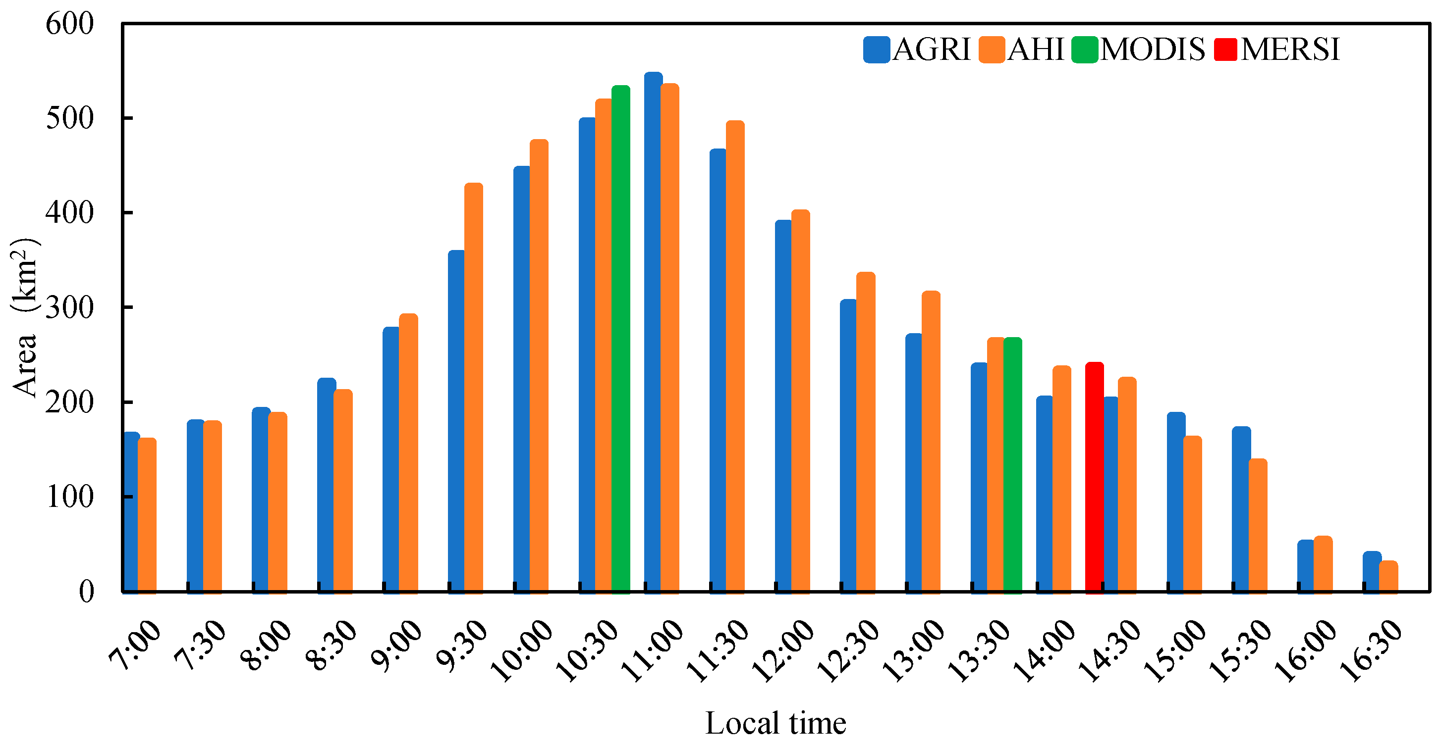
Clearly, the high-frequency measurements provide greater possibilities and better opportunities to observe events occurring in a dynamic aquatic ecosystem, which in turn supports more a precise interpretation of such events that are important for both research and ecosystem management. It can also be seen from the example in Figure 11 that the narrow patches of algae appear in the northwestern coastal areas of the lake at approximately 07:00 LT, which is approximately 3 and 7 h earlier than evident from Terra/MODIS and FY-3D/MERSI, respectively. The subsequent images show that the area of cyanobacterial blooms gradually expands and its intensity gradually increases. Based on such important information elicited from the high-frequency images, agencies charged with ecosystem management could assess whether a cyanobacterial bloom might be about to develop on the large scale and take adequate measures to prevent it from becoming an ecological disaster. However, such diurnal variation in the area and movement of cyanobacteria patches cannot be determined from MODIS (observations twice daily via Aqua and Terra) or MERSI (observations once daily via FY-3D). Additionally, the maximum patch areas of 531 and 520 km2 determined from AGRI and AHI, respectively, are realized at approximately 11:00 LT (Figure 12). Meanwhile, the areas retrieved from FY-3D/MERSI and Aqua/MODIS are only 237 and 263 km2, respectively, which are far below the maximum area because the observation times are not close to 11:00 LT. Conversely, because the observation time of Terra/MODIS (10:30 LT) is close to 11:00 LT, the derived area of the cyanobacterial bloom is 529 km2, i.e., very close to the maximum area. This suggests that it might be inaccurate to use observation results acquired once daily by polar-orbiting satellites to represent the daily maximum or average area of cyanobacterial blooms, which is a method used often in most previous studies. The use of data acquired by polar-orbiting satellites to estimate long-term patterns of cyanobacterial blooms could result in details of the nature, frequency distribution, and biomass of cyanobacterial blooms being missed or underestimated without a sensor such as AGRI to provide ultra-high-frequency observations of floating cyanobacteria. This high-frequency information of cyanobacteria coverage is important both for the early warning of cyanobacterial blooms harmful to drinking water supplies and for improving the scientific understanding of cyanobacteria dynamics.
4. Discussion
4.1. Possible Environmental Factors Influencing the Diurnal Variation in Cyanobacterial Blooms
Previous studies have shown that the occurrence of a cyanobacteria bloom, including the location and extent, is the interaction result between colonies’ buoyancy, mixing intensity, and horizontal migration by currents [32,54,55]. In a large shallow and eutrophic lake such as Lake Taihu, the occurrence of cyanobacterial blooms is quite different and is characterized by rapid changes in situation and extent, likely coming and going without a trace [32,54,55]. Especially in the warm seasons of summer or autumn, as long as the meteorological and hydrological conditions are suitable, a large number of algae groups that already exist in the water body of the lake can float and sink many times in a day; that is, they can “appear” or “disappear” many times every day [32]. We found that the variation in near-surface wind field may be a key factor in triggering the obvious diurnal variation in cyanobacteria blooms in Lake Taihu [56], which is consistent with the results of other studies [54,55]. These studies have noted that cyanobacteria blooms in Lake Taihu usually erupted in specific environmental conditions with calm winds and waves during the warm season. However, quiescent conditions rarely sustain for few hours in a large shallow lake; thus, the cyanobacteria bloom coverage and distribution detected by the satellites or human vision were highly spatiotemporally changeable, frequently presenting as quickly moving patches on the surface. This high variability originated from the wind-induced waves and currents [54,55]. On one hand, the wind-induced wave disturbances increase the probability of collision of cyanobacterial particles in the water column, resulting in an enlarged cyanobacterial cell mass, which increases the buoyancy of the population and quickly floats up to form surface-visible cyanobacterial blooms after the wind-induced wave disturbance. On the other hand, the spatial–temporal distributions of convergence and divergence zones caused by the wind-induced waves change with the change in wind field, resulting in the high spatial–temporal heterogeneity of cyanobacterial blooms in a short time scale.
4.2. Advantages, Limitations, and Future Works
In this study, the observations from the new sensor AGRI onboard the FY-4B geostationary meteorological satellite were applied for the first time to monitor the cyanobacteria blooms in Lake Taihu, China. It was found that after atmospheric correction processing, the FY-4B/AGRI images can effectively detect the characteristics of cyanobacteria blooms. The spatial pattern, area, and degree of coverage of cyanobacteria blooms derived from AGRI images are highly consistent with those derived from the concurrent H8/AHI images. With high-frequency observations from FY-4B/AGRI, we can obtain much more cyanobacteria bloom images than polar-orbiting satellites, which can only provide a limited number of observations once a day, effectively avoiding the problem of polar-orbiting satellites having difficulty obtaining valid data in cloudy (or hazy) weather. Through high-frequency images from AGRI, government managers can also obtain more detailed information on the spatial distribution and movement trends of cyanobacteria blooms in a timely manner, and determine whether it is necessary to issue an early warning of cyanobacteria disaster, which is important for the supply of safe water to cities. Furthermore, using AGRI FVC images, not only the diurnal change in area of the cyanobacteria but also the diurnal change in the spatial pattern of the cyanobacteria can be revealed with greater detail than can be realized using only the measurements of polar-orbiting satellite sensors such as MODIS or MERSI, as Figure 11 demonstrates. Without such high-frequency observations of cyanobacteria, the use of data acquired by these polar-orbiting satellites to estimate long-term patterns of cyanobacterial blooms could result in details of the nature, frequency distribution, and biomass of cyanobacterial blooms being missed or underestimated.
Similar to other geostationary satellites, the performance of FY-4B/AGRI is inferior to that of polar-orbiting satellites in terms of sensitivity and spatial resolution, which makes it difficult to capture the full details of the spatial distribution of cyanobacterial blooms. As shown in Figure 11, more small areas of cyanobacterial bloom patches can be observed in both MODIS and MERSI FVC images than in AGRI FVC images at concurrent times. However, cyanobacteria dynamics researchers may need detailed information about these small cyanobacterial bloom patches, while drinking water supply managers may not, as they tend to focus on large-scale cyanobacteria blooms that can exacerbate water quality degradation. In addition, the AGRI processing method proposed in this study still requires a certain amount of manual interaction to determine the NDVI threshold, which is the most critical step for discerning cyanobacterial blooms [53]. Although the threshold of NDVI > 0 is sometimes used simply to judge whether the water surface is covered with a cyanobacterial bloom, the selected threshold often varies greatly under different weather conditions. In particular, when the density of cyanobacteria in inland turbid water is not great, the threshold of NDVI > 0 will lead to underrating the degree of cyanobacterial blooms [57]. In fact, for the cyanobacteria–water suspension area, some previous studies adopted the value of NDVI < 0 as the threshold to determine the presence of a cyanobacterial bloom in mixed pixels [58,59,60]. The problem of defining an NDVI threshold that is widely applicable for the identification of cyanobacterial blooms requires more direct field measurements for comprehensive verification.
Overall, our results suggest that under the same environmental conditions, the ability to detect variations in surface cyanobacteria is greatly improved because of the much higher sampling frequency of AGRI in comparison with that of polar-orbiting satellite sensors. It is important to provide much-needed information on the dynamics of cyanobacterial blooms for the monitoring and management of aquatic ecosystems within the target region of FY-4B/AGRI. On a broader scale, the approaches and findings of our study may be extended to other inland lakes in which cyanobacteria dominate, such as Lake Dianchi [10], Lake Chaohu, and Lake Erie [15]. Once the cyanobacteria detection model is tuned with local data, similar long-term observations and research can be conducted with little effort and cost. In addition, considering that our current research was mainly focused on providing high-frequency observation information on cyanobacteria blooms to drinking water management departments, we have not differentiated scum from heavy cyanobacteria blooms, which may affect the identification accuracy of cyanobacteria blooms [61]. In future works, we will adopt satellite images with higher spatial resolution to distinguish scum and cyanobacteria blooms to improve the accuracy of water quality detection.
5. Conclusions
Large numbers of accessible satellite remote sensing images, from which the surface vegetation index over water can be derived, can provide valuable information on the density, extent, and potential impact of cyanobacterial blooms. However, optimum observation frequencies cannot be achieved using polar-orbiting satellites, and the acquisition of sufficient effective data cannot be realized in cloudy weather. In recent decades, the spatial resolution of geostationary satellite imagers has improved markedly and the number of geostationary satellites launched with a payload that includes advanced instruments such as AGRI and AHI has increased. Consequently, more high-quality products are available for the monitoring of the water environment of lakes. In this study, measurements acquired by the geostationary satellite imager FY-4B AGRI were used for the first time to detect cyanobacterial blooms in Lake Taihu by retrieving the vegetation index over water. After atmospheric correction for AGRI images, two indicators, NDVI and FVC, which characterize vegetation status, were applied to detect and analyze cyanobacteria blooms. It was found that AC can improve the NDVI values of cyanobacterial blooms in the lake, and that the NDVI values inverted from AGRI were well comparable with those from AHI. The distribution of cyanobacterial blooms derived from AGRI FVC was highly consistent with that derived from both FY-3D and MODIS for concurrent times, and AGRI can provide much greater detail regarding the diurnal variation in the distribution of cyanobacterial blooms owing to its ultra-high temporal resolution (15 min or better). Although the lower spatial resolution of FY-4B/AGRI might lead to the inability to capture the full spatial details of cyanobacterial blooms, its ultra-high-frequency measurements provide the detailed information necessary for the timely and effective management of aquatic ecosystems. For example, with access to detailed information on the spatial distribution of cyanobacterial blooms updated at 15 min intervals, urban water supply managers would have sufficient time to respond should areas of floating algae approach their water intakes, thereby avoiding drinking water pollution. Moreover, ultra-high-frequency data could help researchers better quantify and understand the dynamics of floating algae. Because of its ultra−high-temporal resolution, it is expected that the data products derived from FY-4B/AGRI will be widely used both for routine monitoring tasks and for scientific studies of inland and coastal aquatic ecosystems.
Author Contributions
Conceptualization, Y.L. and X.H. (Xiuzhen Han); methodology, X.H. (Xin Hang), S.L. and Y.L.; validation, X.L., S.Z. and L.S.; writing—original draft preparation, X.H. (Xin Hang); writing—review and editing, Y.L. All authors have read and agreed to the published version of the manuscript.
Funding
This research was supported by the Fengyun Application Pioneering Project (FY-APP-2021.0403) and the National Natural Science Foundation of China (U2242211).
Data Availability Statement
The AGRI data can be download from the website of NSMC (available online: http://satellite.nsmc.org.cn/PortalSite/Data/Satellite.aspx (accessed on 29 November 2022)). The AHI data can be downloaded from the website of JAXA (JAXA Himawari Monitor (P−Tree System). Available online: https://www.eorc.jaxa.jp/ptree/ (accessed on 1 December 2022)).
Acknowledgments
We thank Changyu Hu for providing IT support. We also thank James Buxton for editing the English text of a draft of this manuscript.
Conflicts of Interest
The authors declare no conflict of interest.
References
- Backer, L.C.; Manassaram-Baptiste, D.; LePrell, R.; Bolton, B. Cyanobacteria and algae blooms: Review of health and environmental data from the harmful algal bloom-related illness surveillance system (HABISS) 2007–2011. Toxins 2015, 7, 1048–1064. [Google Scholar] [CrossRef] [PubMed] [Green Version]
- Hughes, S.E.; Marion, J.W. Cyanobacteria Growth in Nitrogen-&Phosphorus-Spiked Water from a Hypereutrophic Reservoir in Kentucky, USA. J. Environ. Prot. 2021, 12, 75–89. [Google Scholar]
- Wang, K.; Razzano, M.; Mou, X.Z. Cyanobacterial blooms alter the relative importance of neutral and selective processes in assembling freshwater bacterioplankton community. Sci. Total Environ. 2020, 706, 135724. [Google Scholar] [CrossRef]
- Wang, K.; Mou, X.; Cao, H.; Struewing, I.; Allen, J.; Lu, J. Co-occurring microorganisms regulate the succession of cyanobacterial harmful algal blooms. Environ. Pollut. 2021, 288, 117682. [Google Scholar] [CrossRef]
- Zhang, Q.; Zhang, Z.; Lu, T.; Peijnenburg, W.J.G.M.; Gillings, M.; Yang, X.; Chen, J.; Penuelas, J.; Zhu, Y.G.; Zhou, N.Y.; et al. Cyanobacterial blooms contribute to the diversity of antibiotic-resistance genes in aquatic ecosystems. Commun. Biol. 2020, 3, 737. [Google Scholar] [CrossRef]
- Schmale, D.G.; Ault, A.P.; Saad, W.; Scott, T.D.; Westwrick, J.A. Perspectives on Harmful Algal Blooms (HABs) and the Cyberbiosecurity of Freshwater Systems. Front. Bioeng. Biotechnol. 2019, 7, 128. [Google Scholar] [CrossRef] [PubMed] [Green Version]
- O’Neila, J.M.; Davisb, T.W.; Burfordb, M.A.; Gobler, C.J. The rise of harmful cyanobacteria blooms: The potential roles of eutrophication and climate change. Harmful Algae 2012, 14, 313–334. [Google Scholar] [CrossRef]
- Paerl, H.W.; Otten, T.G. Harmful Cyanobacterial Blooms: Causes, Consequences, and Controls. Microb. Ecol. 2013, 65, 995–1010. [Google Scholar] [CrossRef]
- Ho, J.C.; Michalak, A.M.; Pahlevan, N. Widespread global increase in intense lake phytoplankton blooms since the 1980s. Nature 2019, 574, 667–670. [Google Scholar] [CrossRef]
- Zhao, H.; Li, J.; Yan, X.; Fang, S.; Du, Y.; Xue, B.; Yu, K.; Wang, C. Monitoring Cyanobacteria Bloom in Dianchi Lake Based on Ground-Based Multispectral Remote-Sensing Imaging: Preliminary Results. Remote Sens. 2021, 13, 3970. [Google Scholar] [CrossRef]
- Wynne, T.T.; Stumpf, R.P.; Pokrzywinski, K.L.; Litaker, R.W.; De Stasio, B.T.; Hood, R.R. Cyanobacterial Bloom Phenology in Green Bay Using MERIS Satellite Data and Comparisons with Western Lake Erie and Saginaw Bay. Water 2022, 14, 2636. [Google Scholar] [CrossRef]
- Hang, X.; Li, Y.; Li, X.; Xu, M.; Sun, L. Estimation of chlorophyll-a concentration in Lake Taihu from Gaofen-1 wide-field-of-view data through a machine learning trained algorithm. J. Meteor. Res. 2022, 36, 208–226. [Google Scholar] [CrossRef]
- Mozafari, Z.; Noori, R.; Siadatmousavi, S.M.; Afzalimehr, H.; Azizpour, J. Satellite-Based Monitoring of Eutrophication in the Earth’s Largest Transboundary Lake. Geohealth 2023, 7, e2022GH000770. [Google Scholar] [CrossRef] [PubMed]
- Modabberi, A.; Noori, R.; Madani, K.; Ehsani, A.H.; Mehr, A.D.; Hooshyaripor, F.; Kløve, B. Caspian Sea is eutrophying: The alarming message of satellite data. Environ. Res. Lett. 2020, 15, 124047. [Google Scholar] [CrossRef]
- Ho, J.C.; Michalak, A.M. Challenges in tracking harmful algal blooms: A synthesis of evidence from Lake Erie. J. Great Lakes Res. 2015, 41, 317–325. [Google Scholar] [CrossRef] [Green Version]
- Ho, J.C.; Stumpf, R.P.; Bridgeman, T.B.; Michalak, A.M. Using Landsat to extend the historical record of lacustrine phytoplankton blooms: A lake Erie case study. Remote Sens. Environ. 2017, 191, 273–285. [Google Scholar] [CrossRef]
- Shi, K.; Zhang, Y.; Qin, B.; Zhou, B. Remote sensing of cyanobacterial blooms in inland waters: Present knowledge and future challenges. Sci. Bull. 2019, 64, 1540–1556. [Google Scholar] [CrossRef] [Green Version]
- Zhang, Y.; Shi, K.; Cao, Z.; Lai, L.; Geng, J.; Yu, K.; Zhan, P.; Liu, Z. Effects of satellite temporal resolutions on the remote derivation of trends in phytoplankton blooms in inland waters. ISPRS J. Photogramm. Remote Sens. 2022, 191, 188–202. [Google Scholar] [CrossRef]
- Chen, X.; Shang, S.; Lee, Z.; Qi, L.; Yan, J.; Li, Y. High-frequency observation of floating algae from AHI on Himawari-8. Remote Sens. Environ. 2019, 227, 151–161. [Google Scholar] [CrossRef]
- Zhang, P.; Zhu, L.; Tang, S.; Gao, L.; Chen, L.; Zheng, W.; Han, X.; Chen, J.; Shao, J. General Comparison of FY-4A/AGRI With Other GEO/LEO Instruments and Its Potential and Challenges in Non-meteorological Applications. Front. Earth Sci. 2019, 6, 224. [Google Scholar] [CrossRef] [Green Version]
- Wang, M.; Zheng, W.; Liu, C. Application of Himawari-8 data with high-frequency observation for Cyanobacteria bloom dynamically monitoring in Lake Taihu. J. Lake Sci. 2017, 29, 1043–1053. [Google Scholar]
- Hu, C.M.; Muller-Karger, F.E.; Taylor, C.; Carder, K.L.; Kelble, C.; Johns, E.; Heil, C.A. Red tide detection and tracing using MODIS fluorescence data: A regional example in SW Florida coastal waters. Remote Sens. Environ. 2005, 97, 311–321. [Google Scholar] [CrossRef]
- Wang, M.; Shi, W.; Tang, J. Water property monitoring and assessment for China’s inland Lake Taihu from MODIS-Aqua measurements. Remote Sens. Environ. 2011, 115, 841–854. [Google Scholar] [CrossRef]
- Lai, L.; Zhang, Y.C.; Jing, Y.Y.; Liu, Z.M. Research progress on remote sensing monitoring of phytoplankton in eutrophic water. J. Lake Sci. 2021, 33, 1299–1314. [Google Scholar] [CrossRef]
- Chen, Y.; Dai, J.F. Extraction methods of cyanobacteria bloom in Lake Taihu based on RS data. J. Lake Sci. 2008, 20, 179–183. [Google Scholar]
- Qi, L.; Hu, C.M.; Lu, Y.C.; Ma, R.H. Spectral analysis and identification of floating algal blooms in oceans and lakes based on HY-1C/D CZI observations. Natl. Remote Sens. Bull. 2023, 27, 157–170. [Google Scholar]
- Baret, F.; Weiss, M.; Lacaze, R.; Camacho, F.; Makhmara, H.; Pacholcyzk, P.; Smets, B. GEOV1: LAI and FAPAR essential climate variables and FCOVER global time series capitalizing over existing products. Part 1: Principles of development and production. Remote Sens. Environ. 2013, 137, 299–309. [Google Scholar] [CrossRef]
- Jia, K.; Liang, S.; Gu, X.; Baret, F.; Wei, X.; Wang, X.; Yao, Y.; Yang, L.; Li, Y. Fractional vegetation cover estimation algorithm for Chinese GF-1 wide field view data. Remote Sens. Environ. 2016, 177, 184–191. [Google Scholar] [CrossRef]
- Riihimäki, H.; Luoto, M.; Heiskanen, J. Estimating fractional cover of tundra vegetation at multiple scales using unmanned aerial systems and optical satellite data. Remote Sens. Environ. 2019, 224, 119–132. [Google Scholar] [CrossRef]
- Shi, K.; Zhang, Y.; Zhou, Y.; Liu, X.; Zhu, G.; Qin, B.; Gao, G. Long-term MODIS observations of cyanobacterial dynamics in Lake Taihu: Responses to nutrient enrichment and meteorological factors. Sci. Rep. 2017, 7, 40326. [Google Scholar] [CrossRef] [Green Version]
- Cai, L.L.; Zhu, G.W.; Zhu, M.Y.; Yang, G.J.; Zhao, L.L. Succession of phytoplankton structure and its relationship with algae bloom in littoral zone of Meiliang Bay, Taihu Lake. Ecol. Sci. 2012, 31, 345–351. [Google Scholar]
- Kong, F.X.; Ma, R.H.; Gao, J.F.; Wu, X.D. The theory and practice of prevention, forecast and warning on cyanobacteria bloom in Lake Taihu. J. Lake Sci. 2009, 21, 314–328. [Google Scholar]
- Gordon, H.R.; Wang, M. Retrieval of water-leaving radiance and aerosol optical thickness over the oceans with SeaWiFS: A preliminary algorithm. Appl. Opt. 1994, 33, 443–452. [Google Scholar] [CrossRef] [PubMed]
- Pahlevan, N.; Mangin, A.; Balasubramanian, S.V.; Smith, B.; Alikas, K.; Arai, K.; Barbosa, C.; Bélanger, S.; Binding, C.; Bresciani, M.; et al. ACIX-Aqua: A global assessment of atmospheric correction methods for Landsat-8 and Sentinel-2 over lakes, rivers, and coastal waters. Remote Sens. Environ. 2021, 258, 112366. [Google Scholar] [CrossRef]
- Fan, Y.; Li, W.; Gatebe, C.K.; Jamet, C.; Zibordi, G.; Schroeder, T.; Stamnes, K. Atmospheric correction over coastal waters using multilayer neural networks. Remote Sens. Environ. 2017, 199, 218–240. [Google Scholar] [CrossRef]
- Vanhellemont, Q.; Ruddick, K. Advantages of high quality SWIR bands for ocean colour processing: Examples from Landsat-8. Remote Sens. Environ. 2015, 161, 89–106. [Google Scholar] [CrossRef] [Green Version]
- Shard, C.; Ashwin, G.; Aswathy, V.K.; Arvind, S.; Singh, R.P. Remote sensing of inland water quality: A hyperspectral perspective. In Hyperspectral Remote Sensing; Elsevier: Amsterdam, The Netherlands, 2020; pp. 197–219. [Google Scholar]
- Vermote, E.F.; Tanré, D.; Deuze, J.L.; Herman, M.; Morcette, J.J. Second simulation of the satellite signal in the solar spectrum, 6S: An overview. IEEE Trans. Geosci. Remote Sens. 1997, 35, 675–686. [Google Scholar] [CrossRef] [Green Version]
- Han, X.; Wang, F.; Han, Y. Fengyun-3D MERSI True Color Imagery Developed for Environmental Applications. J. Meteor. Res. 2019, 33, 914–924. [Google Scholar] [CrossRef]
- Ding, S.; Weng, F. Influences of physical processes and parameters on simulations of TOA radiance at UV wavelengths: Implications for satellite UV instrument validation. J. Meteor. Res. 2019, 33, 264–275. [Google Scholar] [CrossRef]
- Li, S.; Han, X.; Weng, F. Monitoring Land Vegetation from Geostationary Satellite Advanced Himawari Imager (AHI). Remote Sens. 2022, 14, 3817. [Google Scholar] [CrossRef]
- Feng, L. Key issues in detecting lacustrine cyanobacterial bloom using satellite remote sensing. J. Lake Sci. 2021, 33, 647–652. [Google Scholar]
- Matthews, M.W.; Bernard, S.; Robertson, L. An algorithm for detecting trophic status (chlorophyll-a), cyanobacterial-dominance, surface scums and floating vegetation in inland and coastal waters. Remote Sens. Environ. 2012, 124, 637–652. [Google Scholar] [CrossRef]
- Han, X.Z.; Wu, C.Y.; Zheng, W.; Sun, L. Satellite remote sensing of Cyanophyte using observed spectral measurements over the Taihu lake. J. App. Met. Sci. 2012, 21, 724–730. [Google Scholar]
- Duan, H.T.; Zhang, S.X.; Zhang, Y.Z. Cyanobacteria bloom monitoring with remote sensing in Lake Taihu. J. Lake Sci. 2008, 20, 145–152. [Google Scholar]
- Tucker, C.J. Red and photographic infrared linear combinations for monitoring vegetation. Remote Sens. Environ. 1979, 8, 127–150. [Google Scholar] [CrossRef] [Green Version]
- Hu, C. A novel ocean color index to detect floating algae in the global oceans. Remote Sens. Environ. 2009, 113, 2118–2129. [Google Scholar] [CrossRef]
- Zong, J.-M.; Wang, X.-X.; Zhong, Q.-Y.; Xiao, X.-M.; Ma, J.; Zhao, B. Increasing Outbreak of Cyanobacterial Blooms in Large Lakes and Reservoirs under Pressures from Climate Change and Anthropogenic Interferences in the Middle–Lower Yangtze River Basin. Remote Sens. 2019, 11, 1754. [Google Scholar] [CrossRef] [Green Version]
- Tu, Y.; Jia, K.; Wei, X.; Yao, Y.; Xia, M.; Zhang, X.; Jiang, B. A Time-Efficient Fractional Vegetation Cover Estimation Method Using the Dynamic Vegetation Growth Information from Time Series GLASS FVC Product. IEEE Geosci. Remote Sens. Lett. 2020, 17, 1672–1676. [Google Scholar] [CrossRef]
- Wang, J.; Yan, Q.; Tan, X.L.; Zou, Y.J. Vegetation Coverage Dynamics and Its Driving Factors in Inner Mongolia Based on FVC Information Entropy. Forest Res. Manag. 2019, 159–167. [Google Scholar]
- Yan, K.; Gao, S.; Chi, H. Evaluation of the Vegetation-Index-Based Dimidiate Pixel Model for Fractional Vegetation Cover Estimation. IEEE Geosci. Remote Sens. 2021, 99, 1–14. [Google Scholar] [CrossRef]
- Tang, L.; He, M.; Li, X. Verification of fractional vegetation coverage and NDVI of desert vegetation via UAVRS technology. Remote Sens. 2020, 12, 1742. [Google Scholar] [CrossRef]
- Lin, Q.; Hu, C.; Visser, P.M.; Ma, R. Diurnal changes of cyanobacteria blooms in taihu lake as derived from goci observations. Limnol. Oceanogr. 2018, 63, 1711–1726. [Google Scholar]
- Li, W.; Qin, B.Q. Dynamics of spatiotemporal heterogeneity of cyanobacterial blooms in large eutrophic Lake Taihu, China. Hydrobiologia 2019, 833, 81–93. [Google Scholar] [CrossRef]
- Qin, B.; Yang, G.; Ma, J.; Wu, T.; Li, W.; Liu, L.; Deng, J.; Zhou, J. Spatiotemporal Changes of Cyanobacterial Bloom in Large Shallow Eutrophic Lake Taihu, China. Front. Microbiol. 2018, 9, 451. [Google Scholar] [CrossRef] [PubMed] [Green Version]
- Li, Y.C.; Xie, X.P.; Hang, X.; Zhu, X.L.; Huang, S.; Jing, Y.S. Analysis of wind field features causing cyanobacteria bloom in Taihu Lake combined with remote sensing methods. China Environ. Sci. 2016, 36, 525–533. [Google Scholar]
- Hu, C.; Lee, Z.; Ma, R.; Yu, K.; Li, D.; Shang, S. Moderate resolution imaging spectroradiometer (MODIS) observations of cyanobacteria blooms in Taihu Lake, China. J. Geophys. Res. Ocean. 2010, 115, 303–306. [Google Scholar] [CrossRef] [Green Version]
- Xu, J.P.; Zhang, B.; Li, F.; Song, K.S.; Wang, Z.M. Detecting modes of cyanobacteria bloom using MODIS data in Lake Taihu. J. Lake Sci. 2008, 20, 191–195. [Google Scholar]
- Xie, G.Q.; Li, M.; Lu, W.K.; Zhou, W.M.; Yu, L.X.; Li, F.R.; Yang, S.P. Spectral features, remote sensing identification and breaking-out meteorological conditions of algal bloom in Lake Dianchi. J. Lake Sci. 2010, 22, 327–336. [Google Scholar]
- Pan, X.; Yang, Z.; Yang, Y.B.; Sun, Y.X.; Liu, S.Y.; Xie, W.Y.; Li, T.T. Comparison and applicability analysis of methods for extracting cyanobacteria from Lake Taihu based on GF-6 data. J. Lake Sci. 2022, 34, 1866–1876. [Google Scholar]
- Bresciani, M.; Adamo, M.; Carolis, G.D.; Matta, E.; Pasquariello, G.; Vaičiūtė, D.; Giardino, C. Monitoring blooms and surface accumulation of cyanobacteria in the Curonian Lagoon by combining MERIS and ASAR data. Remote Sens. Environ. 2014, 146, 124–135. [Google Scholar] [CrossRef]
Figure 1.
Map of Lake Taihu, China.
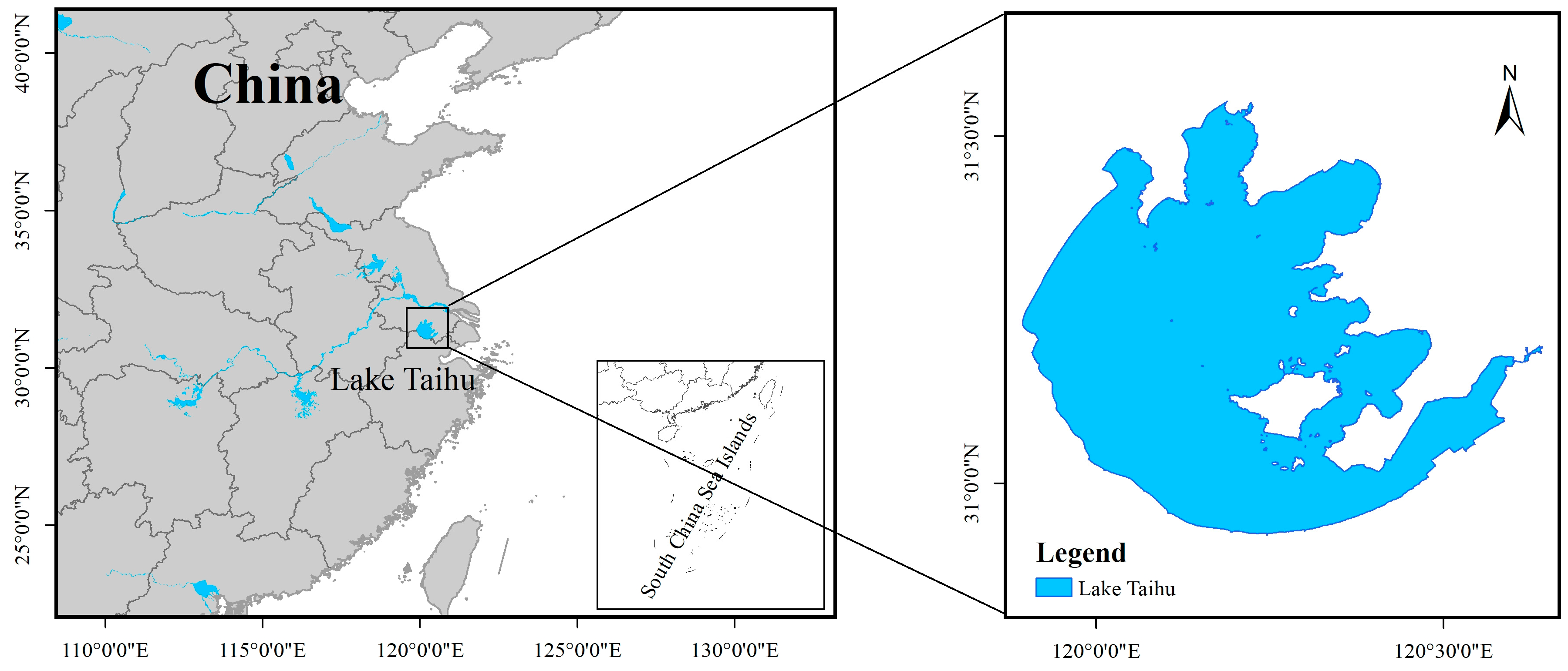
Figure 2.
The technical flow chart of atmospheric correction.
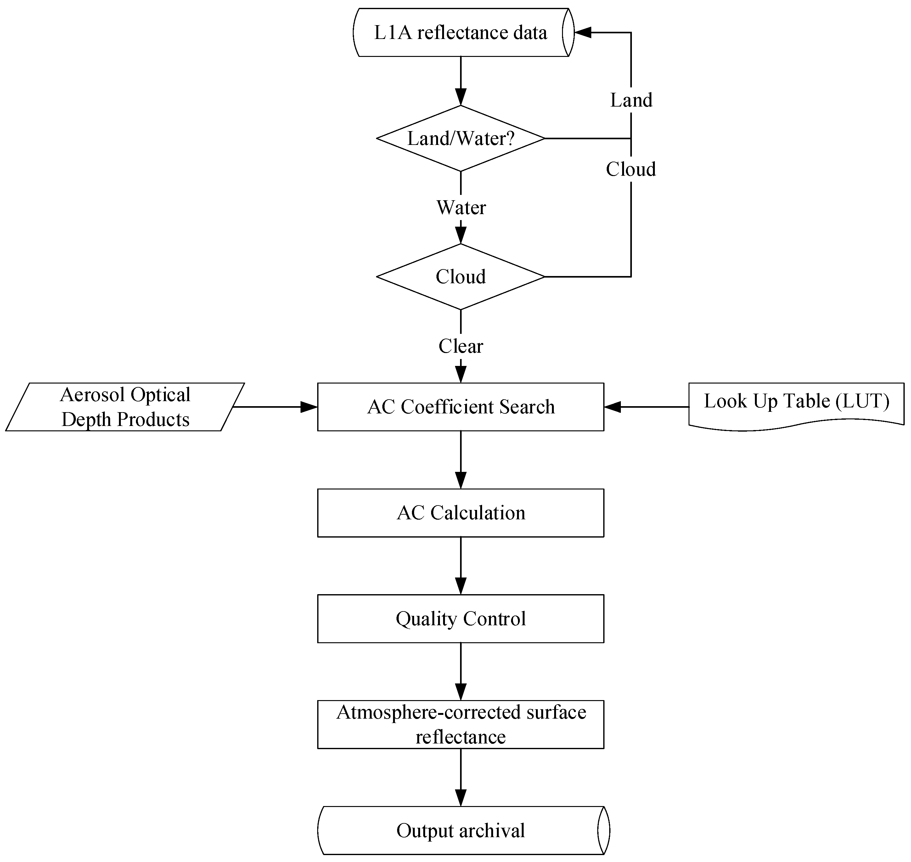
Figure 3.
The AC performance of AGRI observations at 13:00 LT on 1 August 2022: (a) blue, (b) red, and (c) NIR bands. (d–f) are the corresponding scatter plots of (a–c), respectively, with correlation coefficient (r) and averaged percentage error (δ) annotated in the figures. is the atmosphere-corrected reflectance.
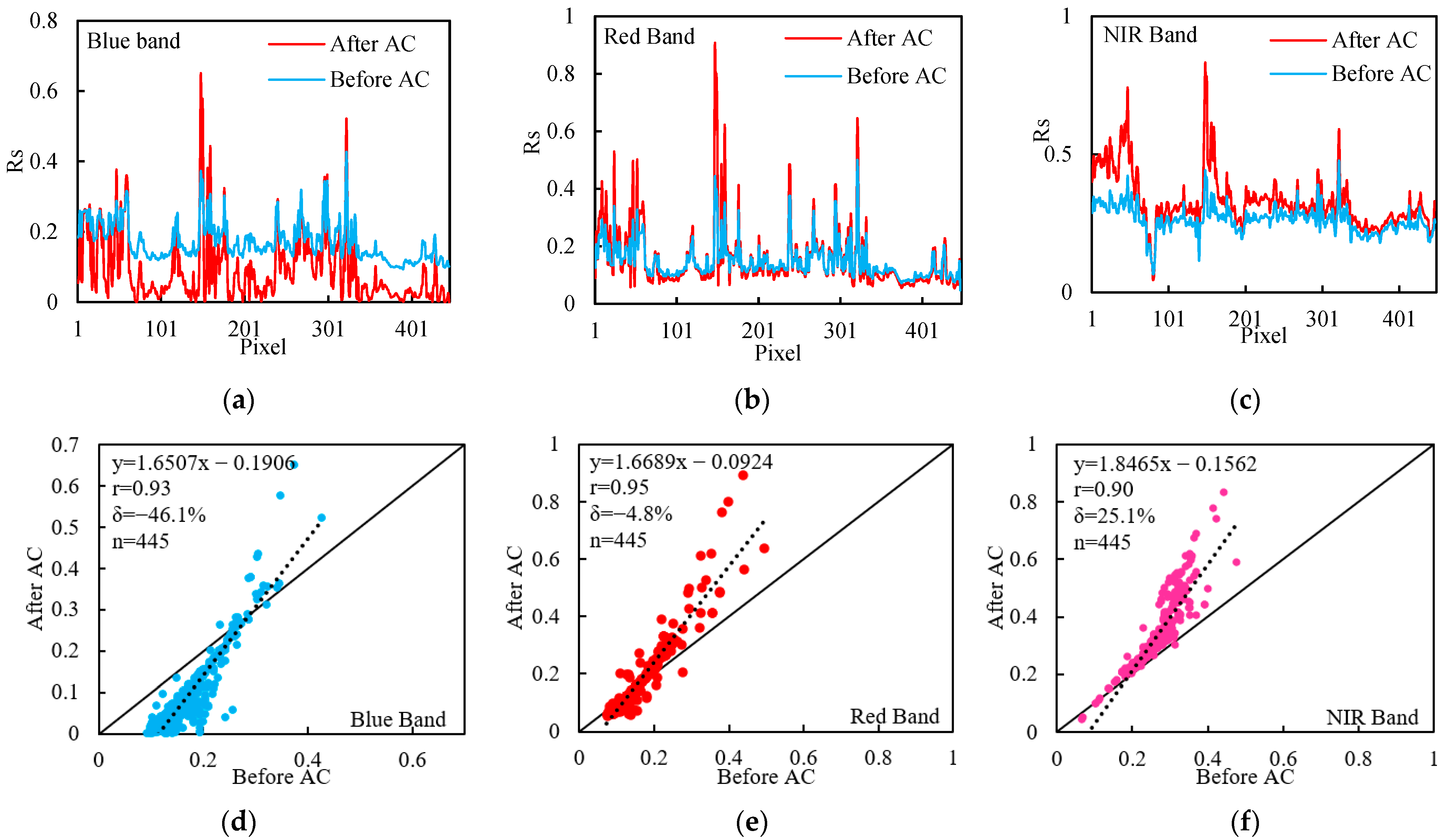
Figure 4.
FY-4B/AGRI false color composite imagery with the band combination of 2:3:1: (a) before AC and (b) after AC.
Figure 4.
FY-4B/AGRI false color composite imagery with the band combination of 2:3:1: (a) before AC and (b) after AC.

Figure 5.
Comparison of AGRI with AHI : (a) blue band, (b) red band, and (c) NIR. The total number of matched points (n) is 2181 for each data pair, and the correlation coefficient (r) and root mean square error (RMSE) values are annotated in each panel. The colored lines are regression lines.
Figure 5.
Comparison of AGRI with AHI : (a) blue band, (b) red band, and (c) NIR. The total number of matched points (n) is 2181 for each data pair, and the correlation coefficient (r) and root mean square error (RMSE) values are annotated in each panel. The colored lines are regression lines.

Figure 6.
In situ reflectance spectra of dense cyanobacteria, cyanobacteria–water, and water observed in Lake Taihu. The spectra were determined as the average spectra of each type of observation target.
Figure 6.
In situ reflectance spectra of dense cyanobacteria, cyanobacteria–water, and water observed in Lake Taihu. The spectra were determined as the average spectra of each type of observation target.
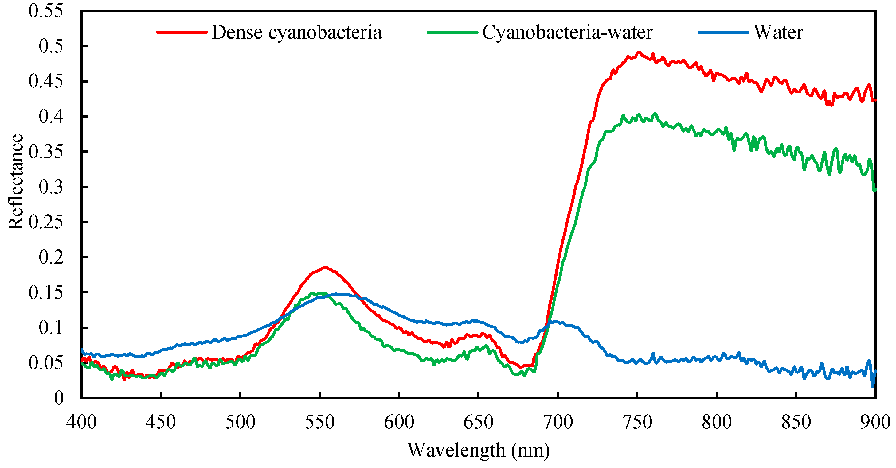
Figure 7.
Comparison of AGRI NDVI before and after AC: (a) all samples, (b) NDVI > 0, (c) −0.2 < NDVI < 0, and (d) NDVI < −0.2 with r, RMSE, and δ annotated in the figures. The solid black lines refer to the 1:1 line and the colored lines are regression lines.
Figure 7.
Comparison of AGRI NDVI before and after AC: (a) all samples, (b) NDVI > 0, (c) −0.2 < NDVI < 0, and (d) NDVI < −0.2 with r, RMSE, and δ annotated in the figures. The solid black lines refer to the 1:1 line and the colored lines are regression lines.
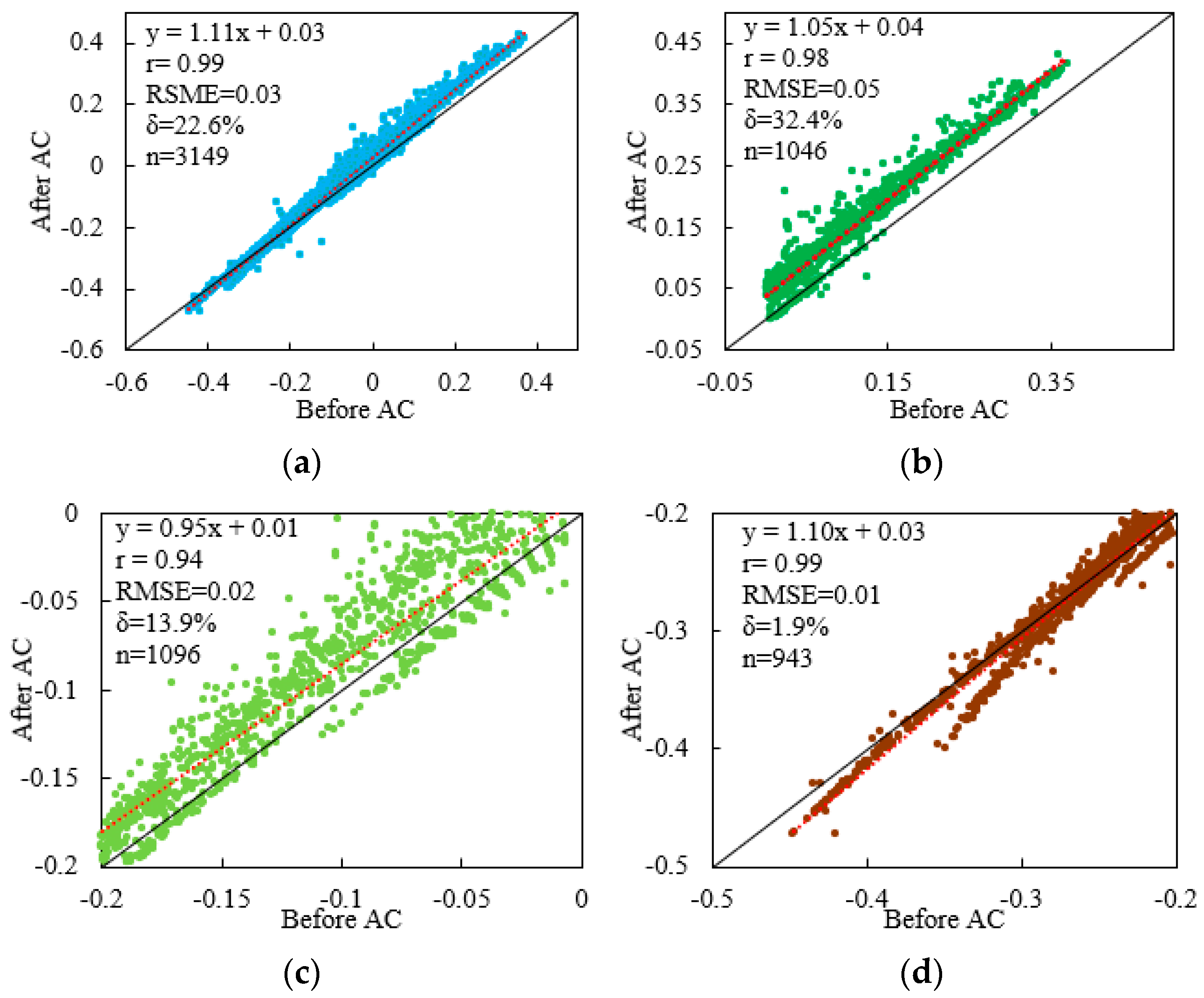
Figure 8.
Comparison between AHI NDVI and AGRI NDVI: (a) before AC and (b) after AC with r, RMSE and δ annotated in the figures. The solid black lines refer to the 1:1 line and the colored lines are regression lines.
Figure 8.
Comparison between AHI NDVI and AGRI NDVI: (a) before AC and (b) after AC with r, RMSE and δ annotated in the figures. The solid black lines refer to the 1:1 line and the colored lines are regression lines.
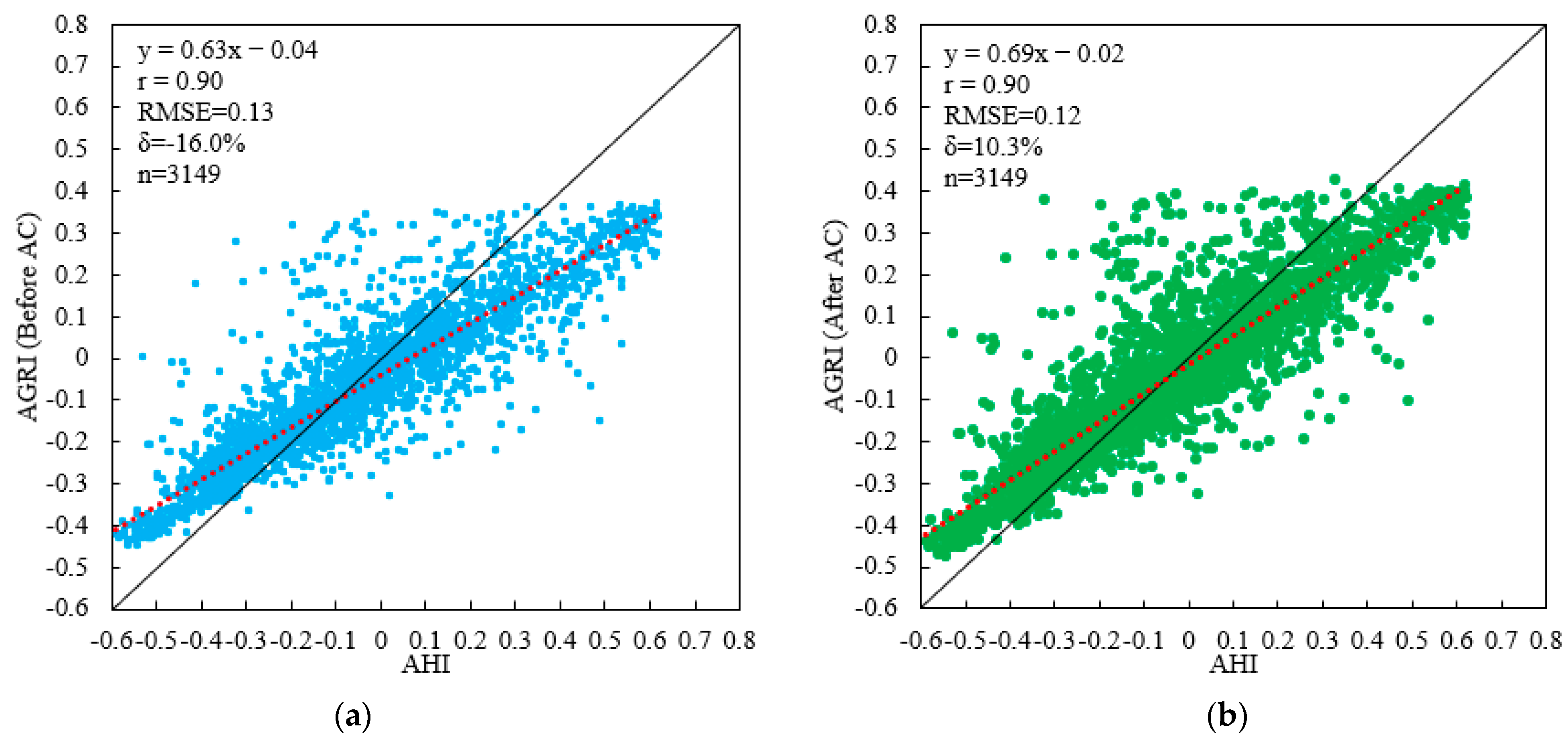
Figure 9.
Cyanobacteria FVCs on 11 October 2022 in Lake Taihu derived from (a) FY-4B/AGRI, (b) H8/AHI, (c) FY-3D/MERSI, and (d) Aqua/MODIS.
Figure 9.
Cyanobacteria FVCs on 11 October 2022 in Lake Taihu derived from (a) FY-4B/AGRI, (b) H8/AHI, (c) FY-3D/MERSI, and (d) Aqua/MODIS.

Figure 10.
Cyanobacteria bloom area in Lake Taihu on 11 October 2022 derived from FY-4B/AGRI and H8/AHI.
Figure 10.
Cyanobacteria bloom area in Lake Taihu on 11 October 2022 derived from FY-4B/AGRI and H8/AHI.

Figure 11.
Cyanobacteria bloom FVCs on 22 October 2022, derived from (a) FY-4B/AGRI, (b) H8/AHI, (c) FY-3D/MERSI, and (d) Terra/Aqua/MODIS.
Figure 11.
Cyanobacteria bloom FVCs on 22 October 2022, derived from (a) FY-4B/AGRI, (b) H8/AHI, (c) FY-3D/MERSI, and (d) Terra/Aqua/MODIS.

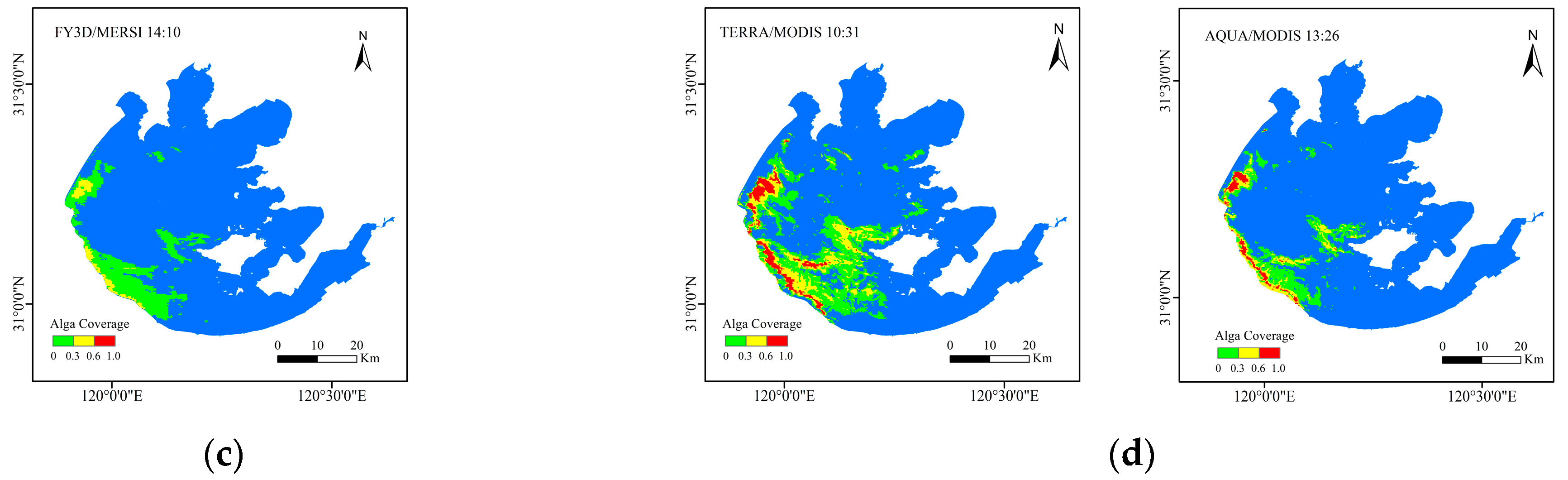
Figure 12.
Cyanobacterial bloom area on 22 October 2022 in Lake Taihu derived from AGRI, AHI, MODIS, and MERSI.
Figure 12.
Cyanobacterial bloom area on 22 October 2022 in Lake Taihu derived from AGRI, AHI, MODIS, and MERSI.

Table 1.
Key specifications of the AGRI sensor.
| Bands | Central Wavelength (μm) | Bandwidth (μm) | Spatial Resolution (km) | SNR |
|---|---|---|---|---|
| 1 | 0.47 | 0.45~0.49 | 1 | S/N ≥ 90 |
| 2 | 0.65 | 0.55~0.75 | 0.5 | S/N ≥ 150 |
| 3 | 0.825 | 0.75~0.90 | 1 | S/N ≥ 200 |
| 4 | 1.379 | 1.371~1.386 | 2 | S/N ≥ 120 |
| 5 | 1.61 | 1.58~1.64 | 2 | S/N ≥ 200 |
| 6 | 2.225 | 2.10~2.35 | 2 | S/N ≥ 200 |
| 7 | 3.75 | 3.50~4.00 (high) | 2 | ≤0.7 K (315 K) |
| 8 | 3.75 | 3.50~4.00 (low) | 4 | 0.2 K (300 K) |
| 9 | 6.25 | 5.80~6.70 | 4 | 0.2 K (300 K) |
| 10 | 6.95 | 6.75~7.15 | 4 | 0.25 K (300 K) |
| 11 | 7.42 | 7.24~7.60 | 4 | 0.25 K (300 K) |
| 12 | 8.55 | 8.3~8.8 | 4 | 0.2 K (300 K) |
| 13 | 10.80 | 10.30~11.30 | 4 | 0.2 K (300 K) |
| 14 | 12.00 | 11.50~12.50 | 4 | 0.2 K (300 K) |
| 15 | 13.3 | 13.00~13.60 | 4 | 0.5 K (300 K) |
Disclaimer/Publisher’s Note: The statements, opinions and data contained in all publications are solely those of the individual author(s) and contributor(s) and not of MDPI and/or the editor(s). MDPI and/or the editor(s) disclaim responsibility for any injury to people or property resulting from any ideas, methods, instructions or products referred to in the content. |
© 2023 by the authors. Licensee MDPI, Basel, Switzerland. This article is an open access article distributed under the terms and conditions of the Creative Commons Attribution (CC BY) license (https://creativecommons.org/licenses/by/4.0/).
Share and Cite
MDPI and ACS Style
Hang, X.; Li, X.; Li, Y.; Zhu, S.; Li, S.; Han, X.; Sun, L. High-Frequency Observations of Cyanobacterial Blooms in Lake Taihu (China) from FY-4B/AGRI. Water 2023, 15, 2165. https://doi.org/10.3390/w15122165
AMA Style
Hang X, Li X, Li Y, Zhu S, Li S, Han X, Sun L. High-Frequency Observations of Cyanobacterial Blooms in Lake Taihu (China) from FY-4B/AGRI. Water. 2023; 15(12):2165. https://doi.org/10.3390/w15122165
Chicago/Turabian StyleHang, Xin, Xinyi Li, Yachun Li, Shihua Zhu, Shengqi Li, Xiuzhen Han, and Liangxiao Sun. 2023. "High-Frequency Observations of Cyanobacterial Blooms in Lake Taihu (China) from FY-4B/AGRI" Water 15, no. 12: 2165. https://doi.org/10.3390/w15122165
Note that from the first issue of 2016, this journal uses article numbers instead of page numbers. See further details here.