Article

Assessment of Three GPM IMERG Products for GIS-Based Tropical Flood Hazard Mapping Using Analytical Hierarchy Process

1
GeoInformatic Unit, Geography Section, School of Humanities, Universiti Sains Malaysia, Gelugor 11800, Penang, Malaysia
2
School of Geography, Nanjing Normal University, Xianlin University District, Nanjing 210023, China
3
Department of Civil Engineering, Faculty of Engineering, Universiti Putra Malaysia, Serdang 43400, Selangor, Malaysia
4
College of Geography and Environmental Sciences, Zhejiang Normal University, Jinhua 321004, China
5
Department of Earth Sciences and Environment, Faculty of Science and Technology, Universiti Kebangsaan Malaysia, Bangi 43600, Selangor, Malaysia
6
River Engineering and Urban Drainage Research Centre (REDAC), Universiti Sains Malaysia, Engineering Campus, Nibong Tebal 14300, Penang, Malaysia
7
Air Syarikat Sdn Bhd, Lot 188, Jln Tuan Guru Nik Abdul Aziz, Kota Bharu 15050, Kelantan, Malaysia
*
Author to whom correspondence should be addressed.
Water 2023, 15(12), 2195; https://doi.org/10.3390/w15122195
Submission received: 24 February 2023 / Revised: 31 May 2023 / Accepted: 6 June 2023 / Published: 11 June 2023
(This article belongs to the Special Issue Remote Sensing-Based Study on Surface Water Environment)

Abstract

:
The use of satellite precipitation products can overcome the limitations of rain gauges in flood hazard mapping for mitigation purposes. Hence, this study aims to evaluate the capabilities of three global precipitation measurement (GPM) integrated multisatellite retrievals for GPM (IMERG) products in tropical flood hazard mapping in the Kelantan River Basin (KRB), Malaysia, using the GIS-based analytic hierarchy process (AHP) method. In addition to the precipitation factor, another eleven factors that contribute to flooding in the KRB were included in the AHP method. The findings demonstrated that the spatial pattern and percentage area affected by floods simulated under the IMERG-Early (IMERG-E), IMERG-Late (IMERG-L), and IMERG-Final (IMERG-F) products did not differ significantly. The receiver operating characteristics curve analysis showed that all three IMERG products performed well in generating flood hazard maps, with area under the curve values greater than 0.8. Almost all the recorded historical floods were placed in the moderate-to-very-high flood hazard areas, with only 1–2% found in the low flood hazard areas. The middle and lower parts of the KRB were identified as regions of “very high” and “high” hazard levels that require particular attention from local stakeholders.

1. Introduction

Floods have an impact on communities across the world in a number of ways, including property damage, loss of life, and the destruction of crops and livestock [1]. According to the United Nations Office for Disaster Risk Reduction (UNDRR), floods are the most common and costly natural disaster in the world, causing more deaths and economic losses than any other natural disaster. The Emergency Events Database of the Centre for Disaster Epidemiology Research (CRED) reported that floods killed 41,816 people and impacted more than 660 million people in Asia between 2010 and 2020, making the region the most disaster-prone in the world [2]. These factors highlight the need of flood hazard mapping for the purpose of planning and mitigating flood damage and risk.
The identification of flood hazard zones is a crucial element of funding allocations, as highlighted by Bubeck et al. [3] and Chapi et al. [4]. To effectively control and reduce floods, flood hazard mapping is a fundamental requirement [5]. Numerous techniques have been developed to study floods, such as frequency ratios [6,7,8], logistic regression modeling [9], artificial neural networks [10,11,12], bivariate statistical approaches [13], time series modeling [14,15,16], and machine learning [17,18]. These techniques are more suitable for flood forecasting, but they may not be able to capture the complex interactions among different factors that contribute to flood risk. The multicriteria decision-making (MCDM) method that combines expert knowledge and multiple factors is regarded as one of the most reliable ways to produce flood hazard maps. This is demonstrated by the 35% increase in publications on the application of MCDM in flood hazard mapping between 2000 and 2019 [19].
Many MCDM methods have been developed with the interfaces of the geographic information system (GIS) [20]. MCDM can be useful in a wide range of considerations when making decisions regarding flood events [21,22,23,24,25]. The climatic, hydrological, lithological, soil, and topographic characteristics of a region have a significant impact on how often flood events occur [26]; hence, flood hazard mapping needs various geospatial data. GIS is a system developed for processing, understanding, organizing, and quantifying a vast amount of geospatial data [27]; therefore, many studies have utilized GIS-based MCDM methods in the field of flood hazard mapping [28,29,30]. The analytical hierarchy process (AHP) is one of the famous MCDM methods to compare multiple criteria pairwise to allow experts’ and decision-makers’ perspectives to be incorporated when producing flood hazard maps for accomplishing targeted goals [31]. Geospatial data of various criteria or factors related to flood risk can be integrated and used as input for the AHP. For example, Rahmati et al. [32] evaluated the effectiveness of the AHP in identifying flood hazard zones by comparing the results with a hydraulic model and reported that the AHP holds promise in accurately and reliably predicting the extent of flood hazards. Such assessment is also required for tropical regions to understand the reliability of the AHP, especially with the complex topography and climatic conditions.
Several studies have produced flood hazard maps using MCDM in Malaysia. Elsheikh et al. [33] and Dano et al. [34] applied different GIS-based MCDM methods to map high-risk flooding areas in Terengganu and Perlis, respectively. They ranked and displayed different categories of very high to no flood risk zones using factors such as annual rainfall, slope, drainage network, and soil type. Both studies relied heavily on the rainfall data measured from gauges as the input to MCDM. Rain gauges are able to provide precise information as they record precipitation as it directly falls on the Earth’s surface [35,36,37,38]. However, rain gauges often have a restricted area of coverage, i.e., mountainous and forest areas. In fact, there are not enough rain gauges in many places around the world to reliably record the spatial and temporal variability of precipitation systems [39,40], particularly over mountainous regions. This situation leads to difficulty in measuring and understanding the impact of rainfall on flooding accurately and effectively. To overcome this challenge, satellite precipitation products (SPPs) can be regarded as alternative climate data to provide rainfall information for regions with limited rain gauges.
Satellite technology has advanced significantly in recent years, making it possible to monitor severe rainfall over large areas at a relatively low cost. As a follow-up mission to the Tropical Rainfall Measuring Mission (TRMM), the National Aeronautics and Space Administration (NASA) and the Japan Aerospace Exploration Agency (JAXA) launched global precipitation measurement (GPM) in 2014 [41]. GPM’s spatial resolution of 0.1° is comparable to TRMM’s spatial resolution of 0.25° [42]. Recent attempts to use GPM to construct a rainfall map and other inputs have been promising [43]. Pradhan et al. [44] reported the integrated multisatellite retrievals for GPM (IMERG) products are able to provide reliable global precipitation information. Ma et al. [45] found that GPM IMERG products are able to increase the reliability of the flash flood warning system in Yunnan province and the nearby area. Similarly, Parsian et al. [46] concluded that flood mapping in Iran can be improved by incorporating GPM IMERG data. However, the assessment of the performance of GPM IMERG products for tropical flood hazard mapping using the AHP method is relatively limited, despite the widespread use of SPPs in monitoring precipitation during the flooding seasons in the past few years. Validating GPM IMERG products in flood hazard mapping is, therefore, crucial to enhance their accuracy and reliability [47]. Additionally, insights from studies will be useful to support the use of SPPs in the GIS-based AHP flood mapping by local stakeholders.
This study aims to assess the reliability of three GPM IMERG products in MCDM to generate flood hazard maps for the Kelantan River Basin (KRB) in Malaysia, which is frequently affected by extreme floods [48]. The most devastating flood events of the basin that occurred in 2014, 2017, and 2020 were selected for the assessment. The findings of this study, including the generated flood hazard maps, can be utilized by stakeholders and decision-makers for flood mitigation strategy development. In addition, the entire framework may be extended to different river basins in Malaysia and nearby countries to generate flood hazard mapping without relying on rainfall data from gauges. This will help local stakeholders to produce flood hazard maps faster as some of the IMERG products, i.e., IMERG-Early (IMERG-E) and IMERG-Late (IMERG-L), are freely available to the public after a few hours of capturing the rainfall pattern.

2. Materials and Methods

2.1. Study Area

The KRB is located in the northeastern region of Peninsular Malaysia between 4°40′ to 6°12′ N latitudes and 101°20′ to 102°20′ E longitudes (Figure 1). The Kelantan River is 248 km in length, with a drainage area of 12,686 km2. The river passes through several populated districts, such as Kuala Krai and Tanah Merah, as well as the state capital, Kota Bharu, before discharging into the South China Sea. The KRB experiences a monsoon climate system, with two major seasons of the northeast monsoon (NEM) from November to March and the southwest monsoon (SEM) from May to September. Meanwhile, April and October are another two inter-monsoon seasons. The KRB receives an average annual precipitation of around 2500 mm (Figure 1), mostly during the early NEM season from November to January. The massive floods in December 2014 and January 2015 caused by monsoon rainfall are considered one of the worst natural catastrophes in Kelantan’s history [49]. The incident caused the displacement of over 200,000 individuals, resulted in the death of 21 people [50]. According to the Department of Irrigation and Drainage Malaysia, the 2014 flood in Kelantan, Malaysia resulted in significant economic losses in the agriculture and infrastructure sectors, estimated at approximately RM 1.5 billion (equivalent to USD 350 million). This estimation reflects the damages incurred due to the flood event.

2.2. Data Description

Several factors were chosen for MCDM modeling after reviewing literature and consulting experts. A model for assessing flood hazards requires identifying parameters related to floods, and there is no consensus on which criteria should be used for this analysis [31,51]. In addition, the selection of criteria should also be based on the availability of data. Rainfall, surface runoff, elevation, distance to rivers, slope, soil type, land use, lithology, road network density, building density, and population density criteria were chosen for their potential importance in relation to flood hazards, as indicated in previous research [52,53]. The process of creating a flood hazard map includes creating a geographic database, integrating spatial data, performing the AHP method, validating the model using historical flood data, and producing the final flood map, as shown in Figure 2. Detailed explanations of these criteria can be found in the following section.

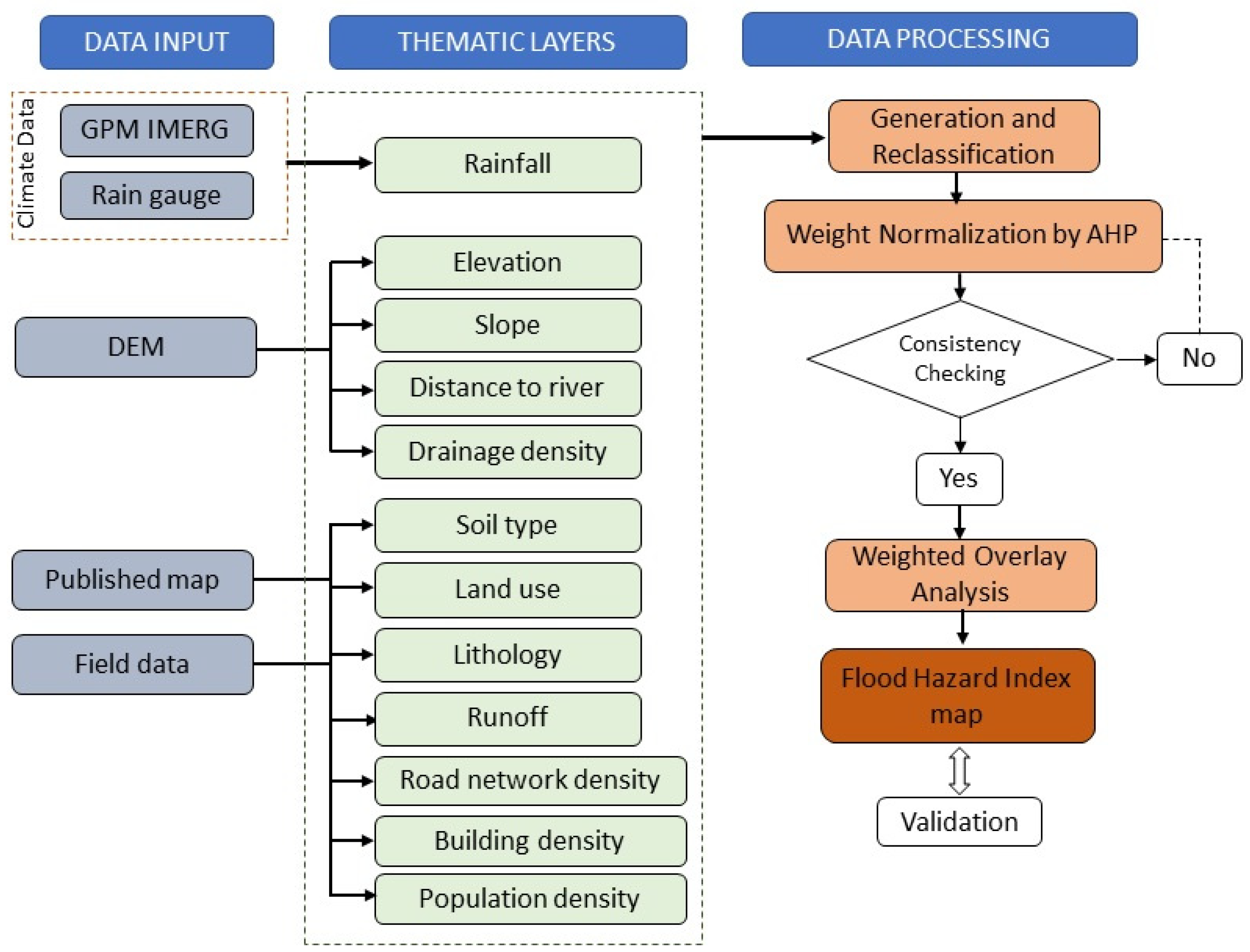
2.3. Data Processing and Analysis

The description and data sources of all the selected criteria, excluding rainfall, are presented in Table 1. The selection of these criteria was based on their significance in relation to the flood hazard in the study area and the quality of the available datasets. The data were processed using ArcGIS 10.6 and projected onto the Kertau RSO Malaya (m) coordinate system to preserve the accuracy of the results and protect the integrity of the study area.

2.4. Selection of Flooding Hazard Factors

The selection of flooding hazard factors and their significance varies among studies, lacking consistency [57,58]. Researchers often choose flooding hazard factors based on the specific physical and natural properties of the study area [59]. In the present study, a comprehensive literature review was conducted to identify and select twelve flood causative factors based on their relevance and significance, as reported in previous research. In addition, the availability of geospatial data is also a major consideration when deciding the use of the factors or variables.
The ArcGIS platform was used to reclassify and rank all the selected criteria from 1 to 5, indicating a very low to a very high flood hazard. The cell sizes were set to minimum units of 30 m × 30 m to capture as much detail as possible on the ground. All the created layers are illustrated in Figure 3a–k. The specific details of each layer are discussed in the following subsections.

2.4.1. Meteorological Data

Rain Gauge Data

Daily observed rainfall data from 25 rain gauges, as shown in Figure 1, for 2014, 2017, and 2020 were collected from Malaysian Meteorological Department (MMD). The rain gauges were distributed across the KRB, with more rain gauges installed in the highly populated areas in the downstream part of the KRB. We generated annual rainfall distribution maps using the inverse distance weighted (IDW) interpolation technique in ArcGIS 10.6. Utilizing a statistical spatial correlation of variables, IDW can predict values at unknown places based on those at known locations [60]. It is well-accepted as one of the most reliable interpolations techniques in rainfall data interpolation.

Satellite Datasets

The GPM IMERG products have full global coverage (60° S~60° N) [37], with spatial resolution of 0.1° × 0.1° and temporal resolution of 30 min. All three different products, (1) IMERG-Early Run (IMERG-E) available with a latency of 4 h, (2) IMERG-Late Run (IMERG-L) available after 12 h of latency, and (3) IMERG-Final Run (IMERG-F), a research product with a latency of 3.5 months [61], were used in flood hazard mapping. The GPM IMERG products can be accessed and downloaded from https://pmm.nasa.gov/dataaccess/downloads/gpm (accessed on 16 January 2022) in NetCDF-4 file format. Annual precipitation data were downloaded and imported into ArcGIS 10.6 using the multidimensional function. The downloaded global precipitation measurement integrated multisatellite retrievals for GPM (GPM IMERG) dataset were reprojected to the Kertau RSO Malaya Meters coordinate system. NetCDF files are widely used for storing multidimensional scientific data, including remote sensing datasets, such as IMERG GPM. To achieve a consistent resolution, the GPM IMERG products were resampled to a 30 m resolution using the bilinear interpolation (BL) method, as recommended by Ulloa et al. [62], who applied the same approach to resample the TRMM 3B43V7 product due to its simplicity. It has been recognized as a common technique to resample SPPs before performing the AHP method [63,64,65]. However, bilinear interpolation may lead to the smoothing of the precipitation field, potentially reducing the precision of the estimates. The effectiveness of the resampling procedure was evaluated by comparing the resampled IMERG data to the original data using general statistical metrics, such as the correlation coefficient (CC), root mean square error (RMSE), and relative bias (RB) [36,66,67,68]. Next, 100 points were created randomly and then compared between resampled IMERG data and the original data. The point-to-grid approach was used to compare GPM IMERG and rain gauges, as most grids were only covered by a single rain gauge [69]. The equations of the statistical metrics are shown as follows:
C C = i = 1 n O i O S i S ¯ i = 1 n ( O i O ¯ ) 2 . i = 1 n S i S ¯ 2
R M S E = i = 1 n O i S i 2 n
R B = i = 1 n S i O i i = 1 n O i ( 100 )
These metrics are derived using the original IMERG (Oi), resampled IMREG (Si), and the number of samples (n). Between −1 and 1, the CC measures the linear relationship between two variables. Strong correlations are shown by values towards 1; weak correlations are denoted by values nearer to 0. To calculate the root mean squared error, the errors’ standard deviations were averaged. The systematic bias between the resampled IMERG data and the original data were evaluated using the relative bias (RB), with the RB represented as a percentage. Resampling operations inherently involve transforming data from one spatial resolution to another, which may lead to the loss or alteration of specific spatial information and cause uncertainties in the final outputs [70]. To further investigate the resampling effects, three resampling techniques, nearest neighbor, bilinear interpolation, and cubic convolution, were used to resample the GPM IMERG-F product to produce the 2014 flood for comparison with the gauge-generated FHI map and historical observed flood events.

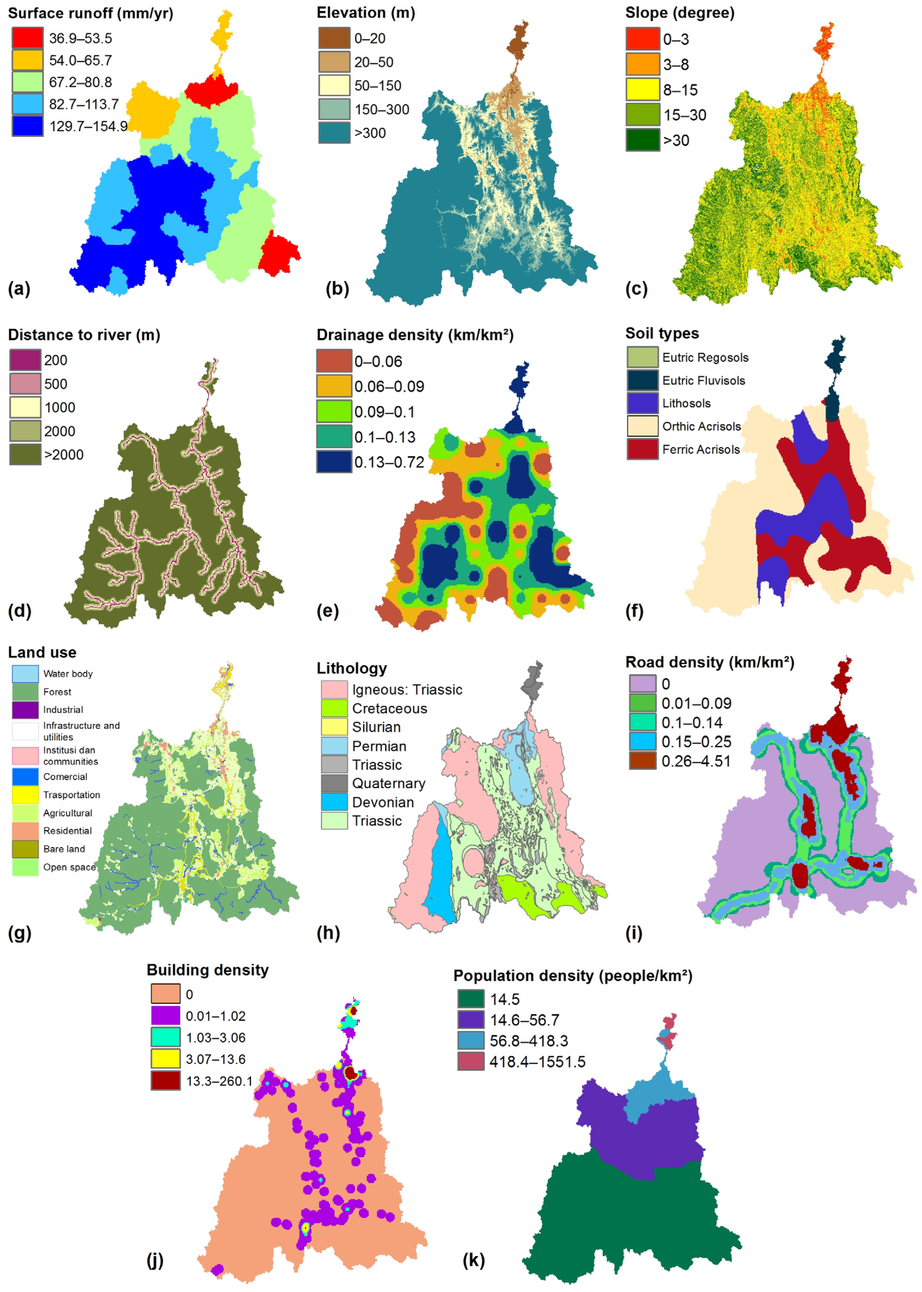
2.4.2. Surface Runoff

Flooding often occurs due to increases in surface runoff, which can contribute to higher flood peaks [71,72]. According to Pradhan et al. [73], floods in Malaysia are caused by monsoons or convective rains, resulting in high surface runoff. The surface runoff data used in this study were derived from the soil and water assessment tool (SWAT) model developed by Tan et al. [54]. A river network was integrated into the 90 m digital elevation model (DEM) using the “burn-in” method for more accurate basin delineation. The model performance in terms of monthly scale simulation at the Jambatan Guillemard Bridge is rated as “very good” for both the calibration (R2 = 0.84 and NSE = 0.72) and validation (R2 = 0.84 and NSE = 0.63) periods. Overall, surface runoff in the KRB ranges from 37.0 to 155.0 mm/year per subbasin, as shown in Figure 3a.

2.4.3. Elevation

Water flow and surface accumulation are both influenced by elevation because of topographic variations [74]. Compared to higher altitudes, which are less likely to flood [75], lower altitudes have a greater potential for runoff and faster water flow [76]. In this study, elevation was determined using the freely available SRTM DEM with a resolution of 30 m. Based on mean elevation, the study region was divided into five primary topographic elevation classes [77]: (1) low-lying (15 m above sea level), (2) rolling (16–30 m), (3) undulating (31–75 m), (4) hilly (76–300 m), and (5) mountainous (>301 m). As shown in Figure 3b, the KRB’s elevation spans from 0 to 2187 m above sea level. The highest peak in the study area, located on the border between Kelantan and Pahang in the southeast, reaches an elevation of over 2000 m. The lowest point in the region, found in the northern part of the KRB, is below 15 m in elevation.

2.4.4. Slope

A slope with a low gradient will lead to water accumulation and slow infiltration, which can increase the risk of flooding [78,79] Both runoff flow and vertical percolation are influenced by the slope of the terrain [32]. In the KRB, the slope ranged from 2 to 74.30 (see Figure 3c) and was classified into six levels: nearly flat (0–3), gently sloping (3–8), sloping (8–15), moderately steep (15–30), and extremely severe (>30), as proposed by Rahmati et al. [32]. The class with the smallest slope range was assigned the highest weight because of the relatively flat terrain, while the class with the largest slope range was given the lowest weight due to its higher runoff potential.

2.4.5. Distance to Rivers

Distance to a river is one factor that can contribute to the risk of flooding. When a river is close to an area, there is a higher chance that the area will be affected by floods during heavy rain or when the river overflows its banks [58,59]. Areas located close to rivers are known as a higher flood risk region because the floodwaters can reach them more quickly. The thematic map generated using ArcMap 10.6 was divided into five categories of 200 m, 500 m, 1000 m, 2000 m, and more than 2000 m (Figure 3d).

2.4.6. Drainage Density

Drainage density refers to the concentration of stream channels in each area. It is typically measured in terms of the number of feet of stream channel per square foot of land [80,81]. As peak flow is affected by drainage density, it is a crucial factor in predicting flood risk [82]. The stream network of the watershed was extracted from DEM using the auto-delineation function in SWAT, with the threshold of 10,000 ha. Then, the drainage density map of the KRB area was prepared using the line density tool in ArcGIS, as indicated in Table 1. The relationship between flooding risk and drainage density is such that as drainage density increases, the risk of flooding decreases, and as drainage density decreases, the risk of flooding increases [83]. The drainage density in the region ranges from 0.06 km/km2 to 0.72 km/km2 and has been categorized into five groups, as shown in Figure 3e.

2.4.7. Soil Type

The Hydrologic Soil Groups (HSGs) established by the United States Department of Agriculture (USDA) categorize soil into four groups: A, B, C, and D. These HSGs serve as a vital tool for hydrological assessments, particularly in the evaluation of soil infiltration and runoff characteristics. This classification is based on the infiltration rate of each soil texture (Table 2). To assess the amount of infiltration occurring in a watershed, soil texture information is used [84,85].

2.4.8. Land Use

In regions where precipitation events impact surface runoff and erosion, land use plays a crucial role in flood management [86]. As flow is inversely proportional to Manning’s n roughness coefficient [87], lower n values correspond to more discharge. Flood-prone locations may be associated with lower Manning’s n values using this strategy. The Manning values of the research region were derived from [88,89]. This analysis categorized land use into five categories (Table 3). Figure 3g demonstrates the land use distribution of these categories across the KRB.

2.4.9. Lithology

Runoff and infiltration are impacted by the porosity and permeability of soil and rock [32,39]. Four categories of rocks may be used to roughly classify the region’s geology: unconsolidated sediments are the first type of rock, followed by extrusive (volcanic) rocks, sedimentary rocks, and granitic rocks (Table 4). Figure 3h shows that igneous rocks may be found along the study’s west and east borders as well as in the middle area. Igneous rocks are found at the west and east borders, as well as in the middle of the study area.

2.4.10. Road Network Density

Impervious surfaces, as defined by the US Geological Survey (USGS), are hard areas that prevent water from penetrating the earth. These surfaces, which include roads, pavements [90,91], and parking lots, can increase the rate of surface runoff by blocking water from infiltrating the ground [67,68]. For this study, the road network density is categorized into five classes, as shown in Figure 3i.

2.4.11. Building Density

As building density, or the number of buildings per unit area, increases, so does the risk of flood disasters [92,93]. A higher building density results in less open space for water to infiltrate into the ground or be absorbed by vegetation, leading to increased surface runoff and flood risks. Furthermore, buildings can obstruct or redirect the flow of water [85,94], leading to increased flood risks in some areas and reduced risks in others. For this study, building density is categorized into five classes, as shown in Figure 3j. Most of the high building density areas can be found in Kota Bharu, which is in the downstream part of the basin, and in Kuala Krai in the middle part of the basin, which is close to the streamflow station.

2.4.12. Population Density

The risk of flooding tends to increase as the population grows in a particular area [95]. This is because the more people there are in an area, the more exposed the area is to flood risks. Similarly, areas with a higher population density tend to have a higher risk of flooding, as there are more people living in a smaller space. This can disproportionately impact residents living in flood-prone locations, who may be burdened because of high population density. Furthermore, growth in population can also impact the amount of solid waste and rubbish that is discarded in drainage systems, which can exacerbate the frequency and intensity of floods if the expansion is uncontrolled or poorly planned [96]. According to this study, population density by district ranged from 14.5 to 1551.5 people per km2, with the city of Kota Bharu in the north of KRB having the most densely populated area, as shown in Figure 3k.

2.5. Assigned Weights of Criterion

The data layers described in Section 2.4 were converted into the raster format to allow the data to be analyzed in a consistent and standardized way. After the data format conversion, it was necessary to reclassify them into five comparable classes. The reclassification process in this study involved creating a reclassification table that considered the effects of different factors on floods. The detailed information regarding these factors is summarized in Table 5. In order to provide a more descriptive analysis, ratings were assigned to the classes within each thematic layer based on their relative importance for flood hazard, which are very high risk (5), high risk (4), moderate risk (3), low risk (2), and very low risk (1). These ratings were determined by incorporating expert knowledge and conducting a comprehensive literature review to ensure that the reclassification accurately reflected the significance of each factor in contributing to flood hazards. Once the reclassification table was defined, it was applied to the input raster to generate the reclassified output raster using the reclassify tool within the spatial analyst extension in ArcGIS.

2.6. Application of Analytical Hierarchy Process (AHP)

AHP is a method for making decisions by breaking down a complex problem into smaller components and using expert judgment to assign relative importance to each element in the hierarchy. This approach relies on expert opinion to identify the most accurate weightings for the criteria in the decision-making process, which ultimately determine the overall weightings for each factor.
A total of 15 local experts, including specialists in hydrology, civil and environmental engineering, and geology, and officers from National Disaster Management Agency (NADMA), were interviewed. The number and distribution of the experts are listed in Table 6. The purpose of the questionnaire was to collect data and insights from these experts to guide the AHP decision-making procedure. Experts or decision-makers were asked to compare each factor with other factors. The purpose was to determine the relative importance or preference between the two elements being compared. For example, if there were three factors of A, B, and C, pairwise comparisons would involve comparing A with B, A with C, and B with C. During the pairwise comparisons, decision makers assigned values on Saaty’s 1–9 scale to express the relative importance or preference. The scale provides nine values representing the degrees of importance or preference, ranging from 1 (equal importance) to 9 (extreme importance) [97].
Then, a (12  ×  12) pairwise comparison matrix for the AHP-based flood hazard mapping was created (Table 7). It is a square matrix where the rows and columns represent the criteria or alternatives being compared, and the values in the matrix represent the relative importance assigned through pairwise comparisons. The AHP technique takes the results of the pairwise comparisons as input, then employs those results to assign relative weights to each criterion. Checking the consistency of judgments are a consistency ratio (CR) and a consistency index (CI), which are computed using Equation (4):
CR = C I R C I
where RI is the random consistency index, and CI is the consistency index, as expressed in Equation (5):
C I = λ m a x n n 1
where λmax is the principal eigenvector computed using eigenvector technique; and n is number of criteria. To proceed with the analysis, a CR of 10% or less is required. A CR score of zero indicates that the consistency of the pairwise comparisons is satisfactory and that the resulting priorities are reliable.

AHP Normalized Pairwise Comparison

Table 7 demonstrates the rankings of the thematic layers and the criteria weightings that were obtained through the AHP analysis in this study. Based on the AHP analysis and ranking values, the weightings assigned to the flood components were determined to be objective, as indicated by a consistency ratio (CR) of 0.09. According to Saaty [97], the consistency ratio (CR) can be used to evaluate the consistency of the weightings assigned by decision makers. A CR value less than 0.1 is desirable, as it indicates a low likelihood that the weightings were assigned randomly. According to the weight values, rainfall was deemed the most significant indicator, with a value of 0.196, followed by surface runoff, elevation, slope, drainage density, distance to rivers, soil type, lithology, land use, road density, building density, and population density, whose relative weights were 0.176, 0.080, 0.055, 0.062, 0.067, 0.111, 0.018, 0.086, 0.035, 0.057, and 0.057 (Table 7), respectively.

2.7. Sensitivity Analysis

AHP may introduce a subjective element in the assignment of weights to the criteria used in decision-making [98]. To address this issue, sensitivity analysis can be used to evaluate the robustness of the final rankings or decisions and identify potential sources of bias in the AHP method. The sensitivity analysis of the rankings or decisions to change criterion weights, which represent subjective judgments, is particularly important [99]. The sensitivity analysis involves examining the effect of small changes in weight values on the rankings or decisions. If the rankings remain unchanged, errors in the estimation of the weights may be insignificant, but if the rankings are sensitive to changes in one or more weights, the accuracy of the weights should be carefully examined. The Stillwell ranking method was employed to validate and examine the sensitivity of results to flood hazard [100]. This approach utilizes two functions as its basis and were defined using the rank sum weight function:
W j R S = n r j + 1 / k = 1 n ( n r k + 1 ) = 2 ( n + 1 r j / n n + 1 )
and reciprocal rank function:
W j R R = 1 r j / k = 1 n 1 r k
where Wj is the normalized weight for the jth criterion, n is the number of criteria under consideration (k = 1, 2… n), and rj is the rank position of the criterion.

2.8. Flood Hazard Index

To calculate the Flood Hazard Index (FHI), a raster calculator was used to combine the different criteria, taking into account their relative weights. The FHI reflects the degree of impact of each component on the risk of flooding, based on the significance of its effect.
To create a flood hazard map, a weighted linear combination (WLC) technique was used to derive the normalized weights of all the data from the pairwise comparison matrix. The constructed method incorporates an FHI into the multicriteria analysis, as shown below:
F H I = i = 1 n Weight × Thematic Layer
The WLC technique is commonly used in flood hazard mapping due to its compatibility with GIS software that has overlay capabilities, allowing for the straightforward application of Equation (8) in the analysis. However, it is important to note that the WLC technique is based on two underlying assumptions [101,102]. The first assumption is linearity, which assumes that the benefit derived from increasing the input of a criterion remains constant and independent of the problem’s characteristics. In other words, the relationship between the criterion and the overall hazard is assumed to be linear. The second assumption is additivity, which assumes that the selected variables or criteria are independent of each other. This implies that the criteria do not interact or depend on one another when contributing to the overall hazard assessment. While the WLC technique offers simplicity and compatibility with GIS software, it is essential to recognize that the linearity and additivity assumptions may not always hold true in real-world scenarios. The relationships between criteria and their contributions to the overall hazard can be nonlinear, and criteria may exhibit interdependencies.
Validation and uncertainty analysis are necessary for assessing the reliability of the generated flood hazard maps [19]. Two techniques, a visual comparison and the receiver operating characteristic (ROC) curve, were employed to determine the reliability of the flood hazard maps. A visual comparison was performed using the ArcGIS’s “extract by mask” function, where the flood hazard maps were compared with the previous flood records. A total of 102 historical floods for the years 2012–2020 were recorded in the flood reports prepared by the Department of Irrigation and Drainage. These historical flood events were rasterized into a map layer format and then overlaid with the flood hazard maps. Then, we calculated the overlapping percentages of “very high” and “high” risk areas generated from the MCDM model with the previous flood events, where 60% of matching indicates the model is acceptable [103]. The second technique was a numerical evaluation based on the ROC curve by considering the area under curve (AUC) value, which has been utilized in numerous flood-related studies [82,83]. The ROC curve between the flood hazard map and actual flood events was calculated using the ArcSDM toolkit. In the ROC analysis, the AUC value ranges from 0.5 to 1.0 [104,105,106]. The accuracy of the model improves as its AUC values increase. An AUC value of 0.5 or lower signifies that the model is appropriate for the study, whereas an AUC value approaching 1 demonstrates the highest level of accuracy.

3. Results

3.1. AHP Sensitivity Analysis

The sensitivity analysis was used to determine how changing the weight values would affect the parameters. Table 8 shows that the rankings of the factors remained relatively stable even when the weight values were altered. The results show that there are no significant changes in the factor ranking even if the values of the weights are changed. This finding suggests that the effect of changes in weight values on the rankings is minimal, validating the accuracy of the final maps. The approach used in this investigation is similar to that used by Souissi et al. [107].

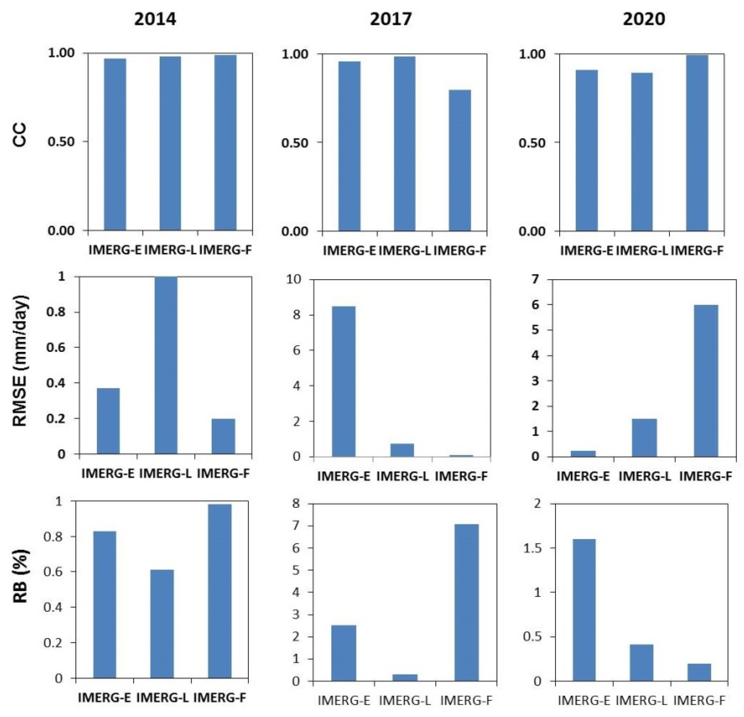
3.2. Statistical Analysis on the Original and Resampled Data of IMERG

Figure 4 presents the statistical analysis comparing the original and resampled IMERG data in the study area. The results demonstrate a strong correlation between the two datasets, with a correlation coefficient above 0.8. The RMSE values of GPM IMERG-E, -L, and -F products ranged from 1.00 to 7.51 mm/month, and the RB values ranged from 1 to 7%. This demonstrates that the resampled data are a reliable representation of the original data and that there is a strong relationship between the two sets of data. Furthermore, a value of relative bias almost close to 0 implies that the resampled data are unbiased and offer an accurate representation of the original data [108].
The 2014 FHI maps generated from the gauges and the IMERG-F product resampled using the nearest neighbor, bilinear, and cubic convolution methods are shown in Figure 5. Upon a visual comparison, no notable variations were found for the generated FHI maps using the three resampling techniques (Table 9), except for the very “high risk” area in the lower part of the basin using the nearest neighbor method. This is consistent with Sliwinski et al. [108], who reported there is no significant difference between the nearest neighbor, bilinear, and cubic methods. Tolche et al. [63] utilized the bilinear method to resample the GPM IMERG-v5 precipitation product to a spatial resolution of 250 m to study the vulnerability of land degradation in the Wabe Shebele River Basin in Ethiopia. As the bilinear method resulted in the closest results to the gauge-generated flood hazard map in identifying the flood locations (Table 9) and is a more common resampling technique in the AHP method, it was selected for FHI mapping in the next steps.

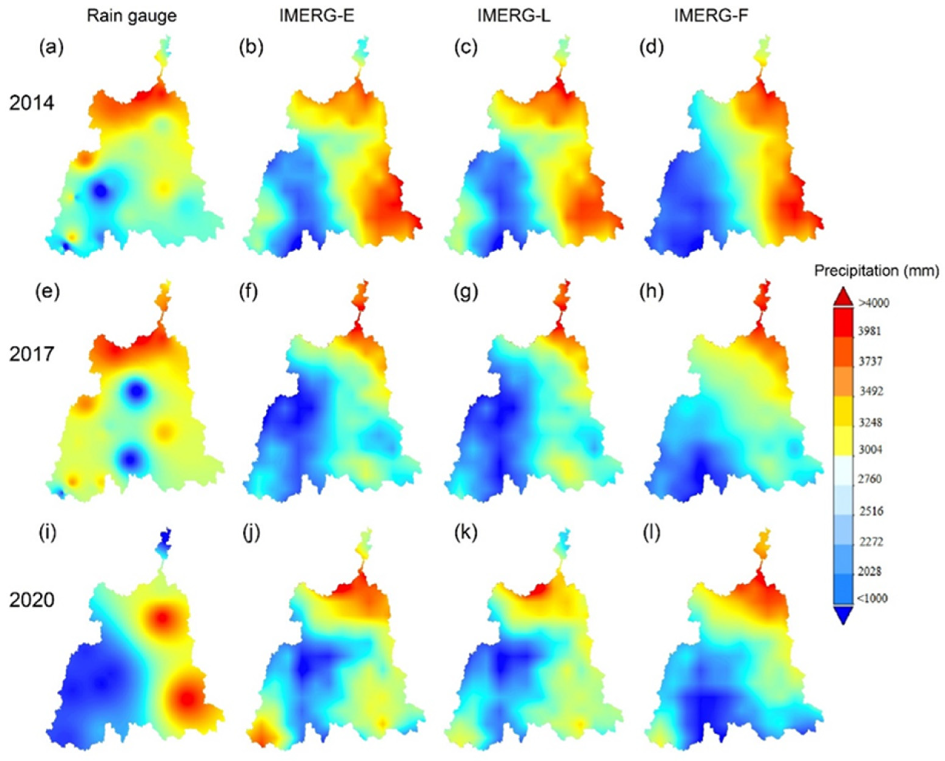
3.3. Spatial Pattern of the IMERG Product and Rain Gauges

The spatial pattern of the total annual precipitation in 2014, 2017, and 2020 of the gauges and three IMERG products is shown in Figure 6. In general, all three IMERG products captured the spatial distribution of the annual precipitation quite well. Regions with a higher precipitation amount are generally found in the northern and eastern regions of the KRB, while lower precipitation is distributed in the western and southern regions. Particularly, all IMERG products capture a very distinct pattern in the area of the South China Sea, represented by slightly higher precipitation totals than the inland areas. These results are similar to those reported by Getirana [109] in Brazil and Tan et al. [110] in Malaysia.
All three IMERG products correlated moderately with the rain gauges in their annual precipitation estimations, with the CC values ranging from 0.61 to 0.63 and the RMSE values from 12.93 to 13.69 mm/day, as listed in Table 10. A moderate correlation in terms of the accuracy and reliability of the products indicates a reasonably good level of agreement between the IMERG data and the reference data used for comparison. The strength of the correlation can vary depending on factors such as regional characteristics, including topography and rainfall intensity [25]. Similar findings were reported by Anjum et al. [111], who advised against using IMERG products in mountainous regions due to the elevated uncertainty in daily precipitation estimates, particularly for light rainfall events.
All the IMERG products overestimated the annual precipitation of the KRB in 2014 and 2020, ranging from 2.78% to 7.02%, while an underestimation of the annual precipitation was found by all three IMERG products in 2017 from 2.03 to 3.21%; IMERG–L underestimated the daily precipitation measured using rain gauges by 10.42 to 17.92%, while IMERG-F showed an overestimation of 7.14%. Similarly, Tan et al. [112] also found GPM IMERG products are able to detect 70% of precipitation and nonprecipitation days, where the detection capability is even higher during flood periods of up to 90%.

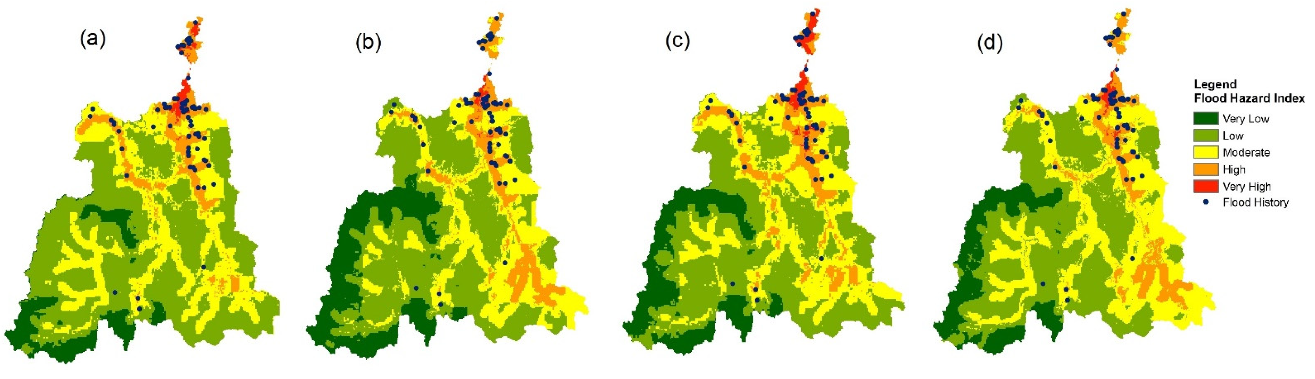
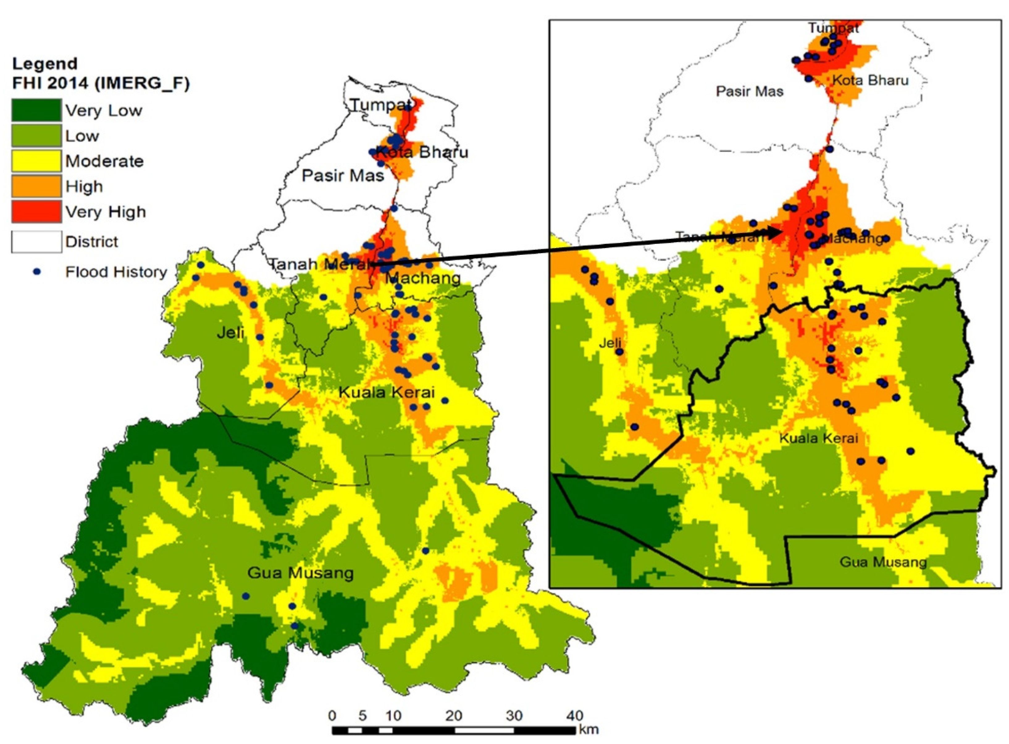
3.4. Validation of Flood Hazard Index

Figure 7 demonstrates ROC curves for a comparison between the actual flood events and flood hazard maps. In general, all flood hazard maps that incorporated the GPM IMERG products performed very well in capturing the actual flooding area, with AUC values of more than 0.90 for the three evaluated flood years. It has been shown that utilizing IMERG as the rainfall input results in accurate flood hazard mapping. The findings indicate that the IMERG products can be used for flood hazard mapping, although they underestimated heavy rainfall during the 2014 flood in the KRB by 4 to 12%, as reported by Tan et al. [110].
The flood hazard maps developed were further confirmed by actual flood events (Table 11). The results indicate that the flood hazard maps and historical data are in good agreement. According to Table 11, most of the recorded flood events are found in high and very high flood hazard regions, ranging from 68 to 78 events and 16 to 29 events, respectively. Subsequently, areas in the moderate class demonstrated 7 to 13 flood events, whereas areas in the low and very low class showed 1 to 2 and 0 flood events, respectively. Almost all the recorded historical floods took place in the moderate to very high flood hazard areas, with only 1–2% of them in areas of low flood hazard.

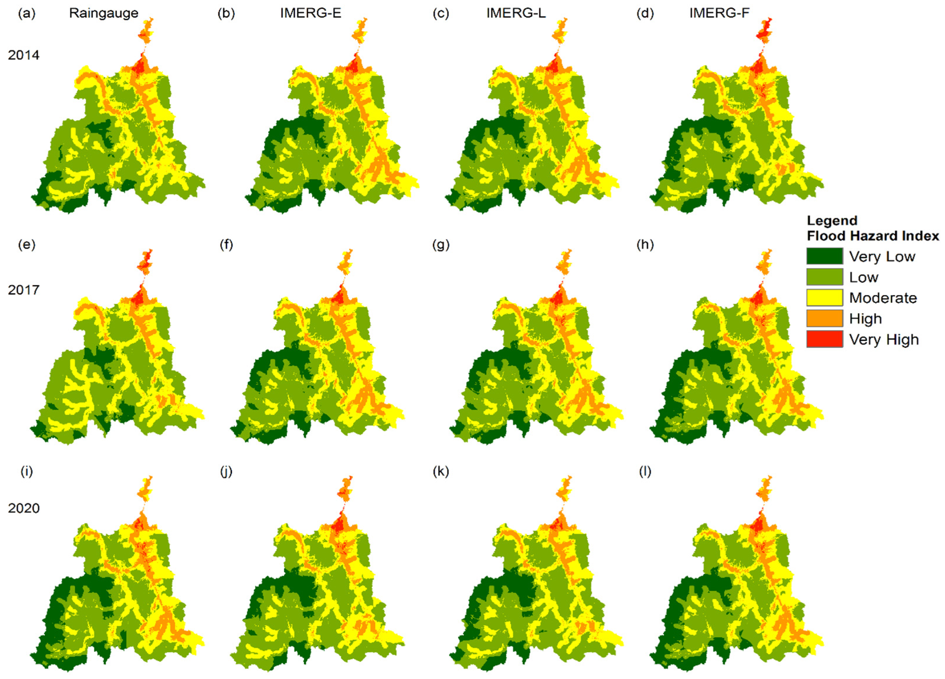
3.5. Flood Hazard Index Mapping

The flood hazard maps generated by the rain gauges and GPM IMERG products are shown in Figure 8. With reference to Figure 8 and Table 11, the FHI distribution using the rain gauges and IMERG does not show significant differences in terms of the number of events at the FHI level of very low, low, moderate, and high. Interestingly, the coverage of the very high flood hazard area tended to be slightly higher under the IMERG-F-simulated FHI maps, particularly during 2014 and 2017. One of the possible explanations might be due to the overestimation of the daily precipitation by IMERG-F in the KRB, while the other two IMERG products tended to underestimate daily precipitation [110]. Analysis of the historical flood data consistently reveals that flood prone areas exhibit common characteristics, including low elevation and proximity to rivers. In the case of the neighboring areas of Tanah Merah and Jeli, these regions are predominantly classified as “very high” due to their flat topography, low elevation, and close proximity to the Galas and Lebir Rivers. This underscores the suitability of using all IMERG products for the generation of hazard index maps. However, it is important to note that there are notable differences in the distribution of the FHI between the rain gauge and IMERG data, particularly in the western and southern regions of the KRB.
The relative proportion of the flood hazard areas for all the five risk classes was calculated and is summarized in Figure 9. On average, the moderate to very high hazard class for KRB contributed a total area of 4778.9 km², equivalent to 37.7% of the total area. The results showed that most of the areas in the very low and low classes were in varying morphological conditions between undulating hills and forests located in the southern part of KRB, which represented about 57.7% (7357.9 km2) of the total area.
Figure 10 shows that the town of Kota Bharu is situated in a very high-risk flooding area. This is due to the fact that Kota Bharu is completely exposed to the potential of monsoon floods occurring due to its proximity to the Kelantan River and its downstream location at the river’s mouth, which goes to the South China Sea. Another reason contributing to the monsoon flood disaster might due to the rapid development of Kota Bharu [113], with its more impervious surface than other regions. The Kuala Kerai district has more high and very high hazard areas, followed by the Machang, Tanah Merah, and Kota Bharu districts. Kuala Krai is the second largest district in Kelantan after Gua Musang. The two main subdistricts of Kuala Krai, Manek Urai and Dabong, are often exposed to floods [114]. In 2014, the Kuala Kerai district experienced a major flood due to the northeast monsoon that brought heavy rain. In addition, the confluence of the Galas and Lebir Rivers in that region also caused flooding [115].

4. Discussion

To effectively address the flood problem, it is crucial to develop a more detailed flood map by incorporating the GIS-based AHP method with the GPM IMERG product as an input for rainfall data [88,89]. Some studies have reported the limitations of IMERG products, such as their inability to accurately depict rapidly changing daily precipitation and the lack of reliable ground-based gauge rainfall information in certain areas [9,110,116]. Additionally, a high variability in precipitation extremes in IMERG grid boxes results in large spatial sampling errors when compared to individual precipitation measurements [117], and the downscaled precipitation products can have inherent systematic biases [118]. Topographic complexity, as noted by Sharifi et al. [119], Yang et al. [120], and Hirpa et al. [121], also adds to this challenge. The IMERG’s ability to detect rainfall events has moderate performance during validation, but its accuracy in flood hazard mapping is comparable to the rain gauge data, i.e., in terms of the differences in spatial patterns and total high-risk areas, as shown in Figure 8 and Figure 9. The validation results showed that IMERG-E and IMERG-L performed slightly better in capturing precipitation patterns compared to the IMERG-F product. This finding is supported by other studies as well [45,122,123,124]. For example, Hou et al. [61] found that the IMERG-E and IMERG-L products that are designed for real-time applications, such as flood monitoring, water management, crop forecasting, and flood mapping, are useful for these purposes. This aligns with the findings of this study.
As per the results presented in Table 10, it was observed that the IMERG products tended to overestimate precipitation in the years 2014 and 2020. Meanwhile, the IMERG products tended to underestimate precipitation in the year 2017. Ebrahimi et al. [66] pointed out that both moderate and heavy rainfalls may be difficult for satellite sensors to detect, which might result in the inadequate monitoring of extreme weather events. Downscaling and interpolating IMERG data might contribute to the errors present in the IMERG data [125]. In addition, the usage of different temporal resolutions (subdaily, daily, and monthly) and flood periods (from when to when) in the GPM IMERG products may also influence the outputs. Therefore, future research should be carried out to establish efficient bias–correction algorithms and to test the sensitivity of different temporal resolutions for improving the entire flood hazard mapping framework.
When used as an input, IMERG can deliver good results when combined with other factors in developing a flood hazard index map. This is proven by most of the recorded flood events area falling within the high and very high-risk flood hazard areas simulated by all three IMERG products. This is consistent with a prior study conducted by Parsian et al. [46], who found IMERG can accurately identify flood risk areas in Pol-e Doktar with about 95% accuracy rate. However, please note that the AHP method requires all geospatial data to be consistent and in the same resolution. Many GIS-based AHP studies have utilized the simple bilinear resampling technique to resample the pixel values of SPPs to a higher resolution [62,63,64,65], but resampling errors might occur, particularly in complex topography and mountainous areas. The minimization of these errors using optimal downscaling techniques, i.e., geographically weighted regression, and cubist and artificial neural networks (ANNs) [126], before applying SPPs in the GIS-based AHP simulations should be considered in the future.
Based on the flood hazard mapping results, it can be observed that the areas that are mostly affected by floods are mainly distributed in the bottom and middle parts of the KRB. This corresponds with the distribution of rainfall, as shown in Figure 6. Town areas are more susceptible to flooding due to inadequate drainage systems that cannot manage the increased runoff, resulting in a higher risk of flooding [127]. The distribution pattern of hazard levels appeared to be significantly different between the upper and lower parts of the KRB. Low land areas with an elevation less than 15 m are more vulnerable to flooding. Low elevation and flat slope angles were among the factors that tended to increase community exposure to flood hazards. The result is compatible with previous studies, such as [77,113,128]. Flooding occurred in the low-lying areas of KRB and affected the districts of Kota Bharu, Tanah Merah, and Kuala Kerai.
The FHI map also showed high and very high hazard class areas located along or near rivers, where the distance from the river was <500 m. Most of the moderate, high, and very high areas were located along the rivers. Pham et al. [129] found that the distance to rivers is the key factor in predicting flash floods. As a result, the distance from rivers was included as a crucial element in creating the FHI map. This highlights that the AHP considers more than just rainfall, as other factors can also contribute to flooding.

5. Conclusions

This research attempts to assess the reliability of three GPM IMERG products in tropical flood hazard mapping using the AHP method, focusing on the Kelantan River Basin (KRB), Malaysia. Rainfall, surface runoff, elevation, drainage density, distance to rivers, slope gradient, soil type, land use, lithology, road density, building density, and population density were identified to be important factors affecting floods in the study area. All these thematic layers were integrated with the IMERG products to generate flood hazard maps for mitigation and planning purposes.
Compared to rain gauges, the GPM IMERG products are able to capture the spatial variability of annual precipitation, where high precipitation regions are in the lower and middle parts of the basin, near the sea, exhibiting the usefulness of alternative precipitation information. However, the AHP requires all the layers to be in the same spatial resolution. High correlations and low biases between the original and resampled GPM IMERG products show that the resampling technique has minimal impact on the outputs, but a more comprehensive assessment should be conducted in the future to understand the influence of different resampling techniques on flood hazard mapping.
Most of the recorded flood events fall in high and very high-risk flooding areas, as simulated using the rain gauges and all three GPM IMERG products. This shows the GPM IMERG products have the potential to be used for tropical flood hazard mapping via the GIS-based AHP method. Interestingly, IMERG-F tended to cover slightly bigger very high-risk areas, particularly in 2014 and 2017. However, the ROC analysis showed all three GPM IMERG products performed well in generating flood hazard maps, with AUC values greater than 0.8.

Author Contributions

Conceptualization, M.L.T.; methodology, M.L.T. and N.S.; validation, N.S.; formal analysis, M.L.T. and N.S.; resources, M.L.T.; data curation, M.L.T., M.H.P.R. and N.S.; writing—original draft preparation, N.S.; writing—review and editing, M.L.T., Z.Z., F.Z., F.T., C.K.C., W.M.M.W.I. and M.H.P.R.; supervision, M.L.T. and W.M.M.W.I.; project administration, M.L.T.; funding acquisition, M.L.T. and F.T. All authors have read and agreed to the published version of the manuscript.

Funding

This research was funded by the Ministry of Higher Education Malaysia via the Long-Term Research Grant Scheme (LRGS) project 2, grant number LRGS/1/2020/UKM-USM/01/6/2, which is under the program of LRGS/1/2020/UKM/01/6.

Data Availability Statement

The flood hazard maps presented in this study are available on request from the corresponding author. However, the raw data are not publicly available as the authors are not the owners of the data and have no right to share the data.

Acknowledgments

Thanks to the Meteorological Department of Malaysia, Department of Irrigation and Drainage Malaysia, PLANMalaysia, Department of Minerals and Geosciences Malaysia, and National Geospatial Centre (PGN) for providing the data in this study.

Conflicts of Interest

The authors declare no conflict of interest.

References

  1. Jonkman, S.N. Global Perspectives on Loss of Human Life Caused by Floods. Nat. Hazards 2005, 34, 151–175. [Google Scholar] [CrossRef]
  2. Cred, U.G. The Human Cost of Disasters: An Overview of the Last 20 Years 2000–2019; United Nations Office for Disaster Risk Reduction: Geneva, Switzerland, 2020. [Google Scholar]
  3. Bubeck, P.; Botzen, W.J.W.; Aerts, J.C.J.H. A Review of Risk Perceptions and Other Factors That Influence Flood Mitigation Behavior. Risk Anal. 2012, 32, 1481–1495. [Google Scholar] [CrossRef] [Green Version]
  4. Chapi, K.; Singh, V.P.; Shirzadi, A.; Shahabi, H.; Bui, D.T.; Pham, B.T.; Khosravi, K. A Novel Hybrid Artificial Intelligence Approach for Flood Susceptibility Assessment. Environ. Model. Softw. 2017, 95, 229–245. [Google Scholar] [CrossRef]
  5. Dung, N.B.; Long, N.Q.; An, D.T.; Minh, D.T. Multi-Geospatial Flood Hazard Modelling for a Large and Complex River Basin with Data Sparsity: A Case Study of the Lam River Basin, Vietnam. Earth Syst. Environ. 2022, 6, 715–731. [Google Scholar] [CrossRef]
  6. Majid, N.A.; Nazi, N.M.; Idris, N.D.M.; Taha, M.R. GIS-Based Livelihood Vulnerability Index Mapping of the Socioeconomy of the Pekan Community. Sustainability 2019, 11, 6935. [Google Scholar] [CrossRef] [Green Version]
  7. Ullah, K.; Zhang, J. GIS-Based Flood Hazard Mapping Using Relative Frequency Ratio Method: A Case Study of Panjkora River Basin, Eastern Hindu Kush, Pakistan. PLoS ONE 2020, 15, e0229153. [Google Scholar] [CrossRef] [PubMed] [Green Version]
  8. Seejata, K.; Yodying, A.; Chatsudarat, S.; Chidburee, P.; Mahavik, N.; Kongmuang, C.; Tantanee, S. Assessment of Flood Hazard Using Geospatial Data and Frequency Ratio Model in Sukhothai Province, Thailand. In Proceedings of the 40th Asian Conference on Remote Sensing, ACRS 2019: Progress of Remote Sensing Technology for Smart Future, Daejeon, Republic of Korea, 14–18 October 2019. [Google Scholar]
  9. Costache, R.; Zaharia, L. Flash-Flood Potential Assessment and Mapping by Integrating the Weights-of-Evidence and Frequency Ratio Statistical Methods in GIS Environment—Case Study: Bâsca Chiojdului River Catchment (Romania). J. Earth Syst. Sci. 2017, 126, 59. [Google Scholar] [CrossRef]
  10. Nandi, A.; Mandal, A.; Wilson, M.; Smith, D. Flood Hazard Mapping in Jamaica Using Principal Component Analysis and Logistic Regression. Environ. Earth Sci. 2016, 75, 465. [Google Scholar] [CrossRef]
  11. Kalantar, B.; Ueda, N.; Saeidi, V.; Janizadeh, S.; Shabani, F.; Ahmadi, K.; Shabani, F. Deep Neural Network Utilizing Remote Sensing Datasets for Flood Hazard Susceptibility Mapping in Brisbane, Australia. Remote Sens. 2021, 13, 2638. [Google Scholar] [CrossRef]
  12. Rahmati, O.; Darabi, H.; Haghighi, A.T.; Stefanidis, S.; Kornejady, A.; Nalivan, O.A.; Bui, D.T. Urban Flood Hazard Modeling Using Self-Organizing Map Neural Network. Water 2019, 11, 2370. [Google Scholar] [CrossRef] [Green Version]
  13. Kabenge, M.; Elaru, J.; Wang, H.; Li, F. Characterizing Flood Hazard Risk in Data-Scarce Areas, Using a Remote Sensing and GIS-Based Flood Hazard Index. Nat. Hazards 2017, 89, 1369–1387. [Google Scholar] [CrossRef]
  14. Abu El-Magd, S.A. Flash Flood Hazard Mapping Using GIS and Bivariate Statistical Method at Wadi Bada’a, Gulf of Suez, Egypt. J. Geosci. Environ. Prot. 2019, 7, 372–385. [Google Scholar] [CrossRef] [Green Version]
  15. Kuenzer, C.; Guo, H.; Huth, J.; Leinenkugel, P.; Li, X.; Dech, S. Flood Mapping and Flood Dynamics of the Mekong Delta: ENVISAT-ASAR-WSM Based Time Series Analyses. Remote Sens. 2013, 5, 687–715. [Google Scholar] [CrossRef] [Green Version]
  16. Sciance, M.B.; Nooner, S.L. Decadal Flood Trends in Bangladesh from Extensive Hydrographic Data. Nat. Hazards 2018, 90, 115–135. [Google Scholar] [CrossRef]
  17. Sghaier, M.O.; Hammami, I.; Foucher, S.; Lepage, R. Flood Extent Mapping from Time-Series SAR Images Based on Texture Analysis and Data Fusion. Remote Sens. 2018, 10, 237. [Google Scholar] [CrossRef] [Green Version]
  18. Norallahi, M.; Seyed Kaboli, H. Urban Flood Hazard Mapping Using Machine Learning Models: GARP, RF, MaxEnt and NB. Nat. Hazards 2021, 106, 119–137. [Google Scholar] [CrossRef]
  19. Mudashiru, R.B.; Sabtu, N.; Abustan, I.; Balogun, W. Flood Hazard Mapping Methods: A Review. J. Hydrol. 2021, 603, 126846. [Google Scholar] [CrossRef]
  20. De Brito, M.M.; Evers, M. Multi-Criteria Decision-Making for Flood Risk Management: A Survey of the Current State of the Art. Nat. Hazards Earth Syst. Sci. 2016, 16, 1019–1033. [Google Scholar] [CrossRef] [Green Version]
  21. De Brito, M.M.; Evers, M.; Delos Santos Almoradie, A. Participatory Flood Vulnerability Assessment: A Multi-Criteria Approach. Hydrol. Earth Syst. Sci. 2018, 22, 373–390. [Google Scholar] [CrossRef] [Green Version]
  22. Malczewski, J.; Rinner, C. Multicriteria Decision Analysis in Geographic Information Science. In Advances in Geographic Information Science; Springer: Berlin/Heidelberg, Germany, 2015. [Google Scholar] [CrossRef]
  23. Skilodimou, H.D.; Bathrellos, G.D.; Alexakis, D.E. Flood Hazard Assessment Mapping in Burned and Urban Areas. Sustainability 2021, 13, 4455. [Google Scholar] [CrossRef]
  24. Zzaman, R.U.; Nowreen, S.; Billah, M.; Islam, A.S. Flood Hazard Mapping of Sangu River Basin in Bangladesh Using Multi-Criteria Analysis of Hydro-Geomorphological Factors. J. Flood Risk Manag. 2021, 14, e12715. [Google Scholar] [CrossRef]
  25. Mahmoody Vanolya, N.; Jelokhani-Niaraki, M. The Use of Subjective–Objective Weights in GIS-Based Multi-Criteria Decision Analysis for Flood Hazard Assessment: A Case Study in Mazandaran, Iran. Geojournal 2021, 86, 379–398. [Google Scholar] [CrossRef]
  26. Pradhan, B. Flood Susceptible Mapping and Risk Area Delineation Using Logistic Regression, GIS and Remote Sensing. J. Spat. Hydrol. 2009, 9, 1–18. [Google Scholar]
  27. Ouma, Y.O.; Tateishi, R. Urban Flood Vulnerability and Risk Mapping Using Integrated Multi-Parametric AHP and GIS: Methodological Overview and Case Study Assessment. Water 2014, 6, 1515–1545. [Google Scholar] [CrossRef] [Green Version]
  28. Youssef, A.M.; Hegab, M.A. Flood-Hazard Assessment Modeling Using Multicriteria Analysis and GIS: A Case Study—Ras Gharib Area, Egypt. In Spatial Modeling in GIS and R for Earth and Environmental Sciences; Elsevier: Amsterdam, The Netherlands, 2019. [Google Scholar]
  29. Ajjur, S.B.; Mogheir, Y.K. Flood Hazard Mapping Using a Multi-Criteria Decision Analysis and GIS (Case Study Gaza Governorate, Palestine). Arab. J. Geosci. 2020, 13, 44. [Google Scholar] [CrossRef]
  30. Ghosh, S.; Das, A. Urban Expansion Induced Vulnerability Assessment of East Kolkata Wetland Using Fuzzy MCDM Method. Remote Sens. Appl. 2019, 13, 191–203. [Google Scholar] [CrossRef]
  31. Tehrany, M.S.; Jones, S.; Shabani, F.; Martínez-Álvarez, F.; Tien Bui, D. A Novel Ensemble Modeling Approach for the Spatial Prediction of Tropical Forest Fire Susceptibility Using LogitBoost Machine Learning Classifier and Multi-Source Geospatial Data. Appl. Clim. 2019, 137, 637–653. [Google Scholar] [CrossRef]
  32. Rahmati, O.; Haghizadeh, A.; Stefanidis, S. Assessing the Accuracy of GIS-Based Analytical Hierarchy Process for Watershed Prioritization; Gorganrood River Basin, Iran. Water Resour. Manag. 2016, 30, 1131–1150. [Google Scholar] [CrossRef]
  33. Elsheikh, R.F.A.; Ouerghi, S.; Elhag, A.R. Flood Risk Map Based on GIS, and Multi Criteria Techniques (Case Study Terengganu Malaysia). J. Geogr. Inf. Syst. 2015, 7, 348–357. [Google Scholar] [CrossRef] [Green Version]
  34. Dano, U.L.; Balogun, A.L.; Matori, A.N.; Yusouf, K.W.; Abubakar, I.R.; Mohamed, M.A.S.; Aina, Y.A.; Pradhan, B. Flood Susceptibility Mapping Using GIS-Based Analytic Network Process: A Case Study of Perlis, Malaysia. Water 2019, 11, 615. [Google Scholar] [CrossRef] [Green Version]
  35. Kidd, C. Satellite Rainfall Climatology: A Review. Int. J. Climatol. 2001, 21, 1041–1066. [Google Scholar] [CrossRef]
  36. Li, J.; Wang, Z.; Wu, X.; Xu, C.Y.; Guo, S.; Chen, X. Toward Monitoring Short-Term Droughts Using a Novel Daily Scale, Standardized Antecedent Precipitation Evapotranspiration Index. J. Hydrometeorol. 2020, 21. [Google Scholar] [CrossRef] [Green Version]
  37. Li, J.; Wang, Z.; Wu, X.; Zscheischler, J.; Guo, S.; Chen, X. A Standardized Index for Assessing Sub-Monthly Compound Dry and Hot Conditions with Application in China. Hydrol Earth Syst Sci 2021, 25. [Google Scholar] [CrossRef]
  38. Villarini, G.; Mandapaka, P.V.; Krajewski, W.F.; Moore, R.J. Rainfall and Sampling Uncertainties: A Rain Gauge Perspective. J. Geophys. Res. Atmos. 2008, 113, D11102. [Google Scholar] [CrossRef]
  39. Xie, X.; Xie, B.; Cheng, J.; Chu, Q.; Dooling, T. A Simple Monte Carlo Method for Estimating the Chance of a Cyclone Impact. Natural Hazards 2021, 107, 2573–2582. [Google Scholar] [CrossRef]
  40. Zhu, G.; Liu, Y.; Wang, L.; Sang, L.; Zhao, K.; Zhang, Z.; Lin, X.; Qiu, D. The Isotopes of Precipitation Have Climate Change Signal in Arid Central Asia. Glob. Planet. Chang 1016, 225, 104103. [Google Scholar] [CrossRef]
  41. Huffman, G.; Bolvin, D.; Braithwaite, D.; Hsu, K.; Joyce, R.; Kidd, C.; Nelkin, E.; Sorooshian, S.; Tan, J.; Xie, P. NASA GPM Integrated Multi-SatellitE Retrievals for GPM (IMERG) Algorithm Theoretical Basis Document (ATBD) Version 06; NASA/GSFC: Greenbelt, MD, USA, 2020; p. 29.
  42. Wang, J.; Petersen, W.A.; Wolff, D.B. Validation of Satellite-Based Precipitation Products from TRMM to GPM. Remote Sens. 2021, 13, 1745. [Google Scholar] [CrossRef]
  43. Das, S.; Gupta, A. Multi-Criteria Decision Based Geospatial Mapping of Flood Susceptibility and Temporal Hydro-Geomorphic Changes in the Subarnarekha Basin, India. Geosci. Front. 2021, 12, 101206. [Google Scholar] [CrossRef]
  44. Pradhan, R.K.; Markonis, Y.; Vargas Godoy, M.R.; Villalba-Pradas, A.; Andreadis, K.M.; Nikolopoulos, E.I.; Papalexiou, S.M.; Rahim, A.; Tapiador, F.J.; Hanel, M. Review of GPM IMERG Performance: A Global Perspective. Remote Sens. Environ. 2022, 268, 112754. [Google Scholar] [CrossRef]
  45. Ma, M.; Wang, H.; Jia, P.; Tang, G.; Wang, D.; Ma, Z.; Yan, H. Application of the GPM-IMERG Products in Flash Flood Warning: A Case Study in Yunnan, China. Remote Sens. 2020, 12, 1954. [Google Scholar] [CrossRef]
  46. Parsian, S.; Amani, M.; Moghimi, A.; Ghorbanian, A.; Mahdavi, S. Flood Hazard Mapping Using Fuzzy Logic, Analytical Hierarchy Process, and Multi-Source Geospatial Datasets. Remote Sens. 2021, 13, 4761. [Google Scholar] [CrossRef]
  47. Jiang, S.; Ren, L.; Xu, C.Y.; Yong, B.; Yuan, F.; Liu, Y.; Yang, X.; Zeng, X. Statistical and Hydrological Evaluation of the Latest Integrated Multi-SatellitE Retrievals for GPM (IMERG) over a Midlatitude Humid Basin in South China. Atmos. Res. 2018, 214, 418–429. [Google Scholar] [CrossRef]
  48. Tan, M.L.; Liang, J.; Samat, N.; Chan, N.W.; Haywood, J.M.; Hodges, K. Hydrological Extremes and Responses to Climate Change in the Kelantan River Basin, Malaysia, Based on the CMIP6 Highresmip Experiments. Water 2021, 13, 1472. [Google Scholar] [CrossRef]
  49. Alias, N.E.; Mohamad, H.; Chin, W.Y.; Yusop, Z. Rainfall Analysis of the Kelantan Big Yellow Flood 2014. J. Teknol. 2016, 78, 83–90. [Google Scholar] [CrossRef] [Green Version]
  50. Baharuddin, K.A.; Wahab, S.F.A.; Rahman, N.H.N.A.; Mohamad, N.A.N.; Kamauzaman, T.H.T.; Noh, A.Y.M.; Majid, M.R.A. The Record-Setting Flood of 2014 in Kelantan: Challenges and Recommendations from an Emergency Medicine Perspective and Why the Medical Campus Stood Dry. Malays. J. Med. Sci. 2015, 22, 1. [Google Scholar]
  51. Xie, X.; Tian, Y.; Wei, G. Deduction of Sudden Rainstorm Scenarios: Integrating Decision Makers’ Emotions, Dynamic Bayesian Network and DS Evidence Theory. Nat. Hazards 2022, 2935–2955. [Google Scholar] [CrossRef]
  52. Shadmehri Toosi, A.; Calbimonte, G.H.; Nouri, H.; Alaghmand, S. River Basin-Scale Flood Hazard Assessment Using a Modified Multi-Criteria Decision Analysis Approach: A Case Study. J. Hydrol. 2019, 574, 660–671. [Google Scholar] [CrossRef]
  53. Seejata, K.; Yodying, A.; Wongthadam, T.; Mahavik, N.; Tantanee, S. Assessment of Flood Hazard Areas Using Analytical Hierarchy Process over the Lower Yom Basin, Sukhothai Province. Procedia Eng. 2018, 212, 340–347. [Google Scholar] [CrossRef]
  54. Tan, M.L.; Ibrahim, A.L.; Yusop, Z.; Chua, V.P.; Chan, N.W. Climate Change Impacts under CMIP5 RCP Scenarios on Water Resources of the Kelantan River Basin, Malaysia. Atmos. Res. 2017, 189, 1–10. [Google Scholar] [CrossRef]
  55. Field, H.L.; Solie, J.B. Introduction to Agricultural Engineering Technology: A Problem Solving Approach; Springer: Berlin/Heidelberg, Germany, 2007. [Google Scholar]
  56. Bunya, S.; Dietrich, J.C.; Westerink, J.J.; Ebersole, B.A.; Smith, J.M.; Atkinson, J.H.; Jensen, R.; Resio, D.T.; Luettich, R.A.; Dawson, C.; et al. A High-Resolution Coupled Riverine Flow, Tide, Wind, Wind Wave, and Storm Surge Model for Southern Louisiana and Mississippi. Part I: Model Development and Validation. Mon. Weather. Rev. 2010, 138, 345–377. [Google Scholar] [CrossRef] [Green Version]
  57. Radmehr, A.; Araghinejad, S. Flood Vulnerability Analysis by Fuzzy Spatial Multi Criteria Decision Making. Water Resour. Manag. 2015, 29, 4427–4445. [Google Scholar] [CrossRef]
  58. Sahana, M.; Patel, P.P. A Comparison of Frequency Ratio and Fuzzy Logic Models for Flood Susceptibility Assessment of the Lower Kosi River Basin in India. Environ. Earth Sci. 2019, 78, 289. [Google Scholar] [CrossRef]
  59. Hu, S.; Cheng, X.; Zhou, D.; Zhang, H. GIS-Based Flood Risk Assessment in Suburban Areas: A Case Study of the Fangshan District, Beijing. Nat. Hazards 2017, 87, 1525–1543. [Google Scholar] [CrossRef]
  60. Singh, S.K.; Srivastava, P.K.; Pandey, A.C. Fluoride Contamination Mapping of Groundwater in Northern India Integrated with Geochemical Indicators and GIS. Water Sci. Technol. Water Supply 2013, 13, 1513–1523. [Google Scholar] [CrossRef]
  61. Hou, A.Y.; Kakar, R.K.; Neeck, S.; Azarbarzin, A.A.; Kummerow, C.D.; Kojima, M.; Oki, R.; Nakamura, K.; Iguchi, T. The Global Precipitation Measurement Mission. Bull. Am. Meteorol. Soc. 2014, 95, 701–722. [Google Scholar] [CrossRef]
  62. Ulloa, J.; Ballari, D.; Campozano, L.; Samaniego, E. Two-Step Downscaling of TRMM 3b43 V7 Precipitation in Contrasting Climatic Regions with Sparse Monitoring: The Case of Ecuador in Tropical South America. Remote Sens. 2017, 9, 758. [Google Scholar] [CrossRef] [Green Version]
  63. Tolche, A.D.; Gurara, M.A.; Pham, Q.B.; Anh, D.T. Modelling and Accessing Land Degradation Vulnerability Using Remote Sensing Techniques and the Analytical Hierarchy Process Approach. Geocarto Int. 2021, 37, 7122–7142. [Google Scholar] [CrossRef]
  64. Sandeep, P.; Reddy, G.P.O.; Jegankumar, R.; Arun Kumar, K.C. Modeling and Assessment of Land Degradation Vulnerability in Semi-Arid Ecosystem of Southern India Using Temporal Satellite Data, AHP and GIS. Environ. Model. Assess. 2021, 26, 143–154. [Google Scholar] [CrossRef]
  65. Malav, L.C.; Yadav, B.; Tailor, B.L.; Pattanayak, S.; Singh, S.V.; Kumar, N.; Reddy, G.P.O.; Mina, B.L.; Dwivedi, B.S.; Jha, P.K. Mapping of Land Degradation Vulnerability in the Semi-Arid Watershed of Rajasthan, India. Sustainability 2022, 14, 10198. [Google Scholar] [CrossRef]
  66. Ebrahimi, S.; Chen, C.; Chen, Q.; Zhang, Y.; Ma, N.; Zaman, Q. Effects of Temporal Scales and Space Mismatches on the TRMM 3B42 v7 Precipitation Product in a Remote Mountainous Area. Hydrol. Process. 2017, 31, 4315–4327. [Google Scholar] [CrossRef]
  67. Chen, Z.; Liu, Z.; Yin, L.; Zheng, W. Statistical Analysis of Regional Air Temperature Characteristics before and after Dam Construction. Urban Clim. 2022, 41, 101085. [Google Scholar] [CrossRef]
  68. Zhang, Y.; Luo, J.; Li, J.; Mao, D.; Zhang, Y.; Huang, Y.; Yang, J. Fast Inverse-Scattering Reconstruction for Airborne High-Squint Radar Imagery Based on Doppler Centroid Compensation. IEEE Trans. Geosci. Remote Sens. 2022, 60, 1–17. [Google Scholar] [CrossRef]
  69. Tan, M.L.; Duan, Z. Assessment of GPM and TRMM Precipitation Products over Singapore. Remote Sens. 2017, 9, 720. [Google Scholar] [CrossRef] [Green Version]
  70. Dai, X. The Effects of Image Misregistration on the Accuracy of Remotely Sensed Change Detection. IEEE Trans. Geosci. Remote Sens. 1998, 36, 1566–1577. [Google Scholar] [CrossRef] [Green Version]
  71. Ab. Ghani, A.; Chang, C.K.; Leow, C.S.; Zakaria, N.A. Sungai Pahang Digital Flood Mapping: 2007 Flood. Int. J. River Basin Manag. 2012, 10, 139–148. [Google Scholar] [CrossRef]
  72. Liu, Y.; Zhang, K.; Li, Z.; Liu, Z.; Wang, J.; Huang, P. A Hybrid Runoff Generation Modelling Framework Based on Spatial Combination of Three Runoff Generation Schemes for Semi-Humid and Semi-Arid Watersheds. J. Hydrol. 2020, 590, 125440. [Google Scholar] [CrossRef]
  73. Pradhan, B.; Youssef, A.M. A 100-Year Maximum Flood Susceptibility Mapping Using Integrated Hydrological and Hydrodynamic Models: Kelantan River Corridor, Malaysia. J. Flood Risk Manag. 2011, 4, 189–202. [Google Scholar] [CrossRef]
  74. Wen, J.; Liu, Q.; Xiao, Q.; Liu, Q.; You, D.; Hao, D.; Wu, S.; Lin, X. Characterizing Land Surface Anisotropic Reflectance over Rugged Terrain: A Review of Concepts and Recent Developments. Remote Sens. 2018, 10, 370. [Google Scholar] [CrossRef] [Green Version]
  75. Fernández, D.S.; Lutz, M.A. Urban Flood Hazard Zoning in Tucumán Province, Argentina, Using GIS and Multicriteria Decision Analysis. Eng. Geol. 2010, 111, 90–98. [Google Scholar] [CrossRef]
  76. Shahabi, H.; Shirzadi, A.; Ghaderi, K.; Omidvar, E.; Al-Ansari, N.; Clague, J.J.; Geertsema, M.; Khosravi, K.; Amini, A.; Bahrami, S.; et al. Flood Detection and Susceptibility Mapping Using Sentinel-1 Remote Sensing Data and a Machine Learning Approach: Hybrid Intelligence of Bagging Ensemble Based on K-Nearest Neighbor Classifier. Remote Sens. 2020, 12, 266. [Google Scholar] [CrossRef] [Green Version]
  77. Nazaruddin, D.A.; Fadilah, N.S.; Zulkarnain, Z. Geological Review of the Rafflesia Trail, Near Kampung Jedip, Lojing Highlands: Inputs for a Nature-Based Tourism Site in Kelantan, Malaysia. J. Trop. Resour. Sustain. Sci. 2015, 3, 86–97. [Google Scholar] [CrossRef]
  78. Towfiqul Islam, A.R.M.; Talukdar, S.; Mahato, S.; Kundu, S.; Eibek, K.U.; Pham, Q.B.; Kuriqi, A.; Linh, N.T.T. Flood Susceptibility Modelling Using Advanced Ensemble Machine Learning Models. Geosci. Front. 2021, 12, 101075. [Google Scholar] [CrossRef]
  79. Bilskie, M.V.; Hagen, S.C. Defining Flood Zone Transitions in Low-Gradient Coastal Regions. Geophys. Res. Lett. 2018, 45, 2761–2770. [Google Scholar] [CrossRef]
  80. Abah, R. Clement An Application of Geographic Information System in Mapping Flood Risk Zones in a North Central City in Nigeria. Afr. J. Environ. Sci. Technol. 2013, 7, 365–371. [Google Scholar] [CrossRef]
  81. Yousefi, S.; Mirzaee, S.; Keesstra, S.; Surian, N.; Pourghasemi, H.R.; Zakizadeh, H.R.; Tabibian, S. Effects of an Extreme Flood on River Morphology (Case Study: Karoon River, Iran). Geomorphology 2018, 304, 30–39. [Google Scholar] [CrossRef]
  82. Zhou, Z.; Stefanon, L.; Olabarrieta, M.; D’Alpaos, A.; Carniello, L.; Coco, G. Analysis of the Drainage Density of Experimental and Modelled Tidal Networks. Earth Surf. Dyn. 2014, 2, 105–116. [Google Scholar] [CrossRef] [Green Version]
  83. Sajedi-Hosseini, F.; Choubin, B.; Solaimani, K.; Cerdà, A.; Kavian, A. Spatial Prediction of Soil Erosion Susceptibility Using a Fuzzy Analytical Network Process: Application of the Fuzzy Decision Making Trial and Evaluation Laboratory Approach. Land Degrad. Dev. 2018, 29, 3092–3103. [Google Scholar] [CrossRef]
  84. Lalitha Muthu, A.C.; Helen Santhi, M. Estimation of Surface Runoff Potential Using SCS-CN Method Integrated with GIS. Indian J. Sci. Technol. 2015, 8, 28. [Google Scholar] [CrossRef] [Green Version]
  85. Qi, B.; Xu, P.; Wu, C. Analysis of the Infiltration and Water Storage Performance of Recycled Brick Mix Aggregates in Sponge City Construction. Water 2023, 15, 363. [Google Scholar] [CrossRef]
  86. Khayyun, T.S.; Alwan, I.A.; Hayder, A.M. Hydrological Model for Hemren Dam Reservoir Catchment Area at the Middle River Diyala Reach in Iraq Using ArcSWAT Model. Appl. Water Sci. 2019, 9, 133. [Google Scholar] [CrossRef] [Green Version]
  87. Vieux, B.E.; Cui, Z.; Gaur, A. Evaluation of a Physics-Based Distributed Hydrologic Model for Flood Forecasting. J. Hydrol. 2004, 298, 155–177. [Google Scholar] [CrossRef]
  88. Chow, V. Bibliography: 1) Handbook of Applied Hydrology. Int. Assoc. Sci. Hydrol. Bull. 1965, 10, 82–83. [Google Scholar] [CrossRef]
  89. Barnes, K.B.; Iii, J.M.M.; Roberge, M.C.; Roberge, M. Impervious Surfaces and the Quality of Natural and Built Environments; Department of Geography and Environmental Planning: Towson, MD, USA, 2002. [Google Scholar]
  90. Starke, P.; Göbel, P.; Coldewey, W.G. Urban Evaporation Rates for Water-Permeable Pavements. Water Sci. Technol. 2010, 62, 1161–1169. [Google Scholar] [CrossRef]
  91. Ma, X.; Dong, Z.; Quan, W.; Dong, Y.; Tan, Y. Real-Time Assessment of Asphalt Pavement Moduli and Traffic Loads Using Monitoring Data from Built-in Sensors: Optimal Sensor Placement and Identification Algorithm. Mech. Syst. Signal Process. 2023, 187. [Google Scholar] [CrossRef]
  92. Barnes, K.B.; Morgan, J.; Roberge, M. Impervious Surfaces and the Quality of Natural and Built Environments; Department of Geography and Environmental Planning, Towson University: Towson, MD, USA, 2001. [Google Scholar]
  93. Sun, R.; Gong, Z.; Gao, G.; Shah, A.A. Comparative Analysis of Multi-Criteria Decision-Making Methods for Flood Disaster Risk in the Yangtze River Delta. Int. J. Disaster Risk Reduct. 2020, 51, 101768. [Google Scholar] [CrossRef]
  94. Wang, G.; Zhao, B.; Lan, R.; Liu, D.; Wu, B.; Li, Y.; Li, Q.; Zhou, H.; Liu, M.; Liu, W.; et al. Experimental Study on Failure Model of Tailing Dam Overtopping under Heavy Rainfall. Lithosphere 2022, 2022, 5922501. [Google Scholar] [CrossRef]
  95. Eigenbrod, F.; Bell, V.A.; Davies, H.N.; Heinemeyer, A.; Armsworth, P.R.; Gaston, K.J. The Impact of Projected Increases in Urbanization on Ecosystem Services. Proc. R. Soc. B Biol. Sci. 2011, 278, 3201–3208. [Google Scholar] [CrossRef] [Green Version]
  96. Hsu, M.H.; Chen, S.H.; Chang, T.J. Inundation Simulation for Urban Drainage Basin with Storm Sewer System. J. Hydrol. 2000, 234, 21–37. [Google Scholar] [CrossRef] [Green Version]
  97. Saaty, T.L. How to Make a Decision: The Analytic Hierarchy Process. Eur. J. Oper. Res. 1990, 48, 9–26. [Google Scholar] [CrossRef]
  98. Kazakis, N.; Kougias, I.; Patsialis, T. Assessment of Flood Hazard Areas at a Regional Scale Using an Index-Based Approach and Analytical Hierarchy Process: Application in Rhodope-Evros Region, Greece. Sci. Total Environ. 2015, 538, 555–563. [Google Scholar] [CrossRef]
  99. Yahaya, S. Multicriteria Analysis for Flood Vulnerable Areas in Hadejia-Jama’are River Basin, Nigeria. In Proceedings of the American Society for Photogrammetry and Remote Sensing—ASPRS Annual Conference 2008—Bridging the Horizons: New Frontiers in Geospatial Collaboration, Portland, OR, USA, 28 April–2 May 2008; Volume 2, pp. 777–785. [Google Scholar]
  100. Stillwell, W.G.; Seaver, D.A.; Edwards, W. A Comparison of Weight Approximation Techniques in Multiattribute Utility Decision Making. Organ. Behav. Hum. Perform. 1981, 28, 62–77. [Google Scholar] [CrossRef]
  101. Eastman, J.R. Idrisi for Windows, Version 2.0: Tutorial Exercises, Graduate School of Geography; Clark University: Worcester, MA, USA, 1997. [Google Scholar]
  102. Malczewski, J. On the Use of Weighted Linear Combination Method in GIS: Common and Best Practice Approaches. Trans. GIS 2000, 4, 5–22. [Google Scholar] [CrossRef]
  103. Bandira, P.N.A.; Mahamud, M.A.; Samat, N.; Tan, M.L.; Chan, N.W. Gis-Based Multi-Criteria Evaluation for Potential Inland Aquaculture Site Selection in the George Town Conurbation, Malaysia. Land 2021, 10, 1174. [Google Scholar] [CrossRef]
  104. Souissi, D.; Souie, A.; Sebei, A.; Mahfoudhi, R.; Zghibi, A.; Zouhri, L.; Amiri, W.; Ghanmi, M. Flood Hazard Mapping and Assessment Using Fuzzy Analytic Hierarchy Process and GIS Techniques in Takelsa, Northeast Tunisia. Arab. J. Geosci. 2022, 15, 1405. [Google Scholar] [CrossRef]
  105. Arabameri, A.; Rezaei, K.; Cerdà, A.; Conoscenti, C.; Kalantari, Z. A Comparison of Statistical Methods and Multi-Criteria Decision Making to Map Flood Hazard Susceptibility in Northern Iran. Sci. Total Environ. 2019, 660, 443–445. [Google Scholar] [CrossRef]
  106. Nandi, A.; Shakoor, A. A GIS-Based Landslide Susceptibility Evaluation Using Bivariate and Multivariate Statistical Analyses. Eng. Geol. 2010, 110, 11–20. [Google Scholar] [CrossRef]
  107. Souissi, D.; Zouhri, L.; Hammami, S.; Msaddek, M.H.; Zghibi, A.; Dlala, M. GIS-Based MCDM–AHP Modeling for Flood Susceptibility Mapping of Arid Areas, Southeastern Tunisia. Geocarto Int. 2020, 35, 991–1017. [Google Scholar] [CrossRef]
  108. Śliwiński, D.; Konieczna, A.; Roman, K. Geostatistical Resampling of LiDAR-Derived DEM in Wide Resolution Range for Modelling in SWAT: A Case Study of Zgłowiączka River (Poland). Remote Sens. 2022, 14, 1281. [Google Scholar] [CrossRef]
  109. Getirana, A.; Kirschbaum, D.; Mandarino, F.; Ottoni, M.; Khan, S.; Arsenault, K. Potential of GPM IMERG Precipitation Estimates to Monitor Natural Disaster Triggers in Urban Areas: The Case of Rio de Janeiro, Brazil. Remote Sens. 2020, 12, 4095. [Google Scholar] [CrossRef]
  110. Tan, M.L.; Santo, H. Comparison of GPM IMERG, TMPA 3B42 and PERSIANN-CDR Satellite Precipitation Products over Malaysia. Atmos. Res. 2018, 202, 63–76. [Google Scholar] [CrossRef]
  111. Anjum, M.N.; Ding, Y.; Shangguan, D.; Ahmad, I.; Ijaz, M.W.; Farid, H.U.; Yagoub, Y.E.; Zaman, M.; Adnan, M. Performance Evaluation of Latest Integrated Multi-Satellite Retrievals for Global Precipitation Measurement (IMERG) over the Northern Highlands of Pakistan. Atmos. Res. 2018, 205, 134–146. [Google Scholar] [CrossRef]
  112. Tan, M.L.; Samat, N.; Chan, N.W.; Roy, R. Hydro-Meteorological Assessment of Three GPM Satellite Precipitation Products in the Kelantan River Basin, Malaysia. Remote Sens. 2018, 10, 1011. [Google Scholar] [CrossRef] [Green Version]
  113. Pah, T.; Syed, R.; Ismail, H. Perubahan Gunatanah Dan Kejadian Banjir di Lembangan Saliran Kelantan. Geogr. Malays. J. Soc. Space 2016, 12, 118–128. [Google Scholar]
  114. Hadi, L.A.; Naim, W.M.; Adnan, N.A.; Nisa, A.; Said, E.S. GIS Based Multi-Criteria Decision Making for Flood Vulnerability Index Assessment. J. Telecommun. Electron. Comput. Eng. 2017, 9, 7–11. [Google Scholar]
  115. Rincón, D.; Khan, U.T.; Armenakis, C. Flood Risk Mapping Using GIS and Multi-Criteria Analysis: A Greater Toronto Area Case Study. Geosciences 2018, 8, 275. [Google Scholar] [CrossRef] [Green Version]
  116. Veloria, A.; Perez, G.J.; Tapang, G.; Comiso, J. Improved Rainfall Data in the Philippines through Concurrent Use of GPM IMERG and Ground-Based Measurements. Remote Sens. 2021, 13, 2859. [Google Scholar] [CrossRef]
  117. Da Silva, N.A.; Webber, B.G.M.; Matthews, A.J.; Feist, M.M.; Stein, T.H.M.; Holloway, C.E.; Abdullah, M.F.A.B. Validation of GPM IMERG Extreme Precipitation in the Maritime Continent by Station and Radar Data. Earth Space Sci. 2021, 8, e2021EA001738. [Google Scholar] [CrossRef]
  118. Chen, C.; Hu, B.; Li, Y. Easy-to-Use Spatial Random-Forest-Based Downscaling-Calibration Method for Producing Precipitation Data with High Resolution and High Accuracy. Hydrol. Earth Syst. Sci. 2021, 25, 5667–5682. [Google Scholar] [CrossRef]
  119. Sharifi, E.; Steinacker, R.; Saghafian, B. Assessment of GPM-IMERG and Other Precipitation Products against Gauge Data under Different Topographic and Climatic Conditions in Iran: Preliminary Results. Remote Sens. 2016, 8, 135. [Google Scholar] [CrossRef] [Green Version]
  120. Yang, M.; Liu, G.; Chen, T.; Chen, Y.; Xia, C. Evaluation of GPM IMERG Precipitation Products with the Point Rain Gauge Records over Sichuan, China. Atmos. Res. 2020, 246, 105101. [Google Scholar] [CrossRef]
  121. Hirpa, F.A.; Gebremichael, M.; Hopson, T. Evaluation of High-Resolution Satellite Precipitation Products over Very Complex Terrain in Ethiopia. J. Appl. Meteorol. Clim. 2010, 49, 1044–1051. [Google Scholar] [CrossRef]
  122. Fang, J.; Yang, W.; Luan, Y.; Du, J.; Lin, A.; Zhao, L. Evaluation of the TRMM 3B42 and GPM IMERG Products for Extreme Precipitation Analysis over China. Atmos. Res. 2019, 223, 24–38. [Google Scholar] [CrossRef]
  123. Wei, G.; Lü, H.; Crow, W.T.; Zhu, Y.; Wang, J.; Su, J. Evaluation of Satellite-Based Precipitation Products from IMERG V04A and V03D, CMORPH and TMPA with Gauged Rainfall in Three Climatologic Zones in China. Remote Sens. 2018, 10, 30. [Google Scholar] [CrossRef] [Green Version]
  124. Asong, Z.E.; Razavi, S.; Wheater, H.S.; Wong, J.S. Evaluation of Integrated Multisatellite Retrievals for GPM (IMERG) over Southern Canada against Ground Precipitation Observations: A Preliminary Assessment. J. Hydrometeorol. 2017, 18, 1033–1050. [Google Scholar] [CrossRef]
  125. Zhao, N.; Jiao, Y. A New HASM-Based Downscaling Method for High-Resolution Precipitation Estimates. Remote Sens. 2021, 13, 2693. [Google Scholar] [CrossRef]
  126. Abdollahipour, A.; Ahmadi, H.; Aminnejad, B. A review of downscaling methods of satellite-based precipitation estimates. Earth Sci. Inform. 2022, 15, 1–20. [Google Scholar] [CrossRef]
  127. Seenirajan, M.; Natarajan, M.; Thangaraj, R.; Bagyaraj, M. Study and Analysis of Chennai Flood 2015 Using GIS and Multicriteria Technique. J. Geogr. Inf. Syst. 2017, 9, 126–140. [Google Scholar] [CrossRef] [Green Version]
  128. Mohamad Radhi, A.; Rohasliney, H.; Zarul, H. Fish Composition and Diversity in Perak, Galas and Kelantan Rivers (Malaysia) after the Major Flood of 2014. Transylv. Rev. Syst. Ecol. Res. 2017, 19, 41–56. [Google Scholar] [CrossRef] [Green Version]
  129. Pham, B.T.; Avand, M.; Janizadeh, S.; Van Phong, T.; Al-Ansari, N.; Ho, L.S.; Das, S.; Van Le, H.; Amini, A.; Bozchaloei, S.K.; et al. GIS Based Hybrid Computational Approaches for Flash Flood Susceptibility Assessment. Water 2020, 12, 683. [Google Scholar] [CrossRef] [Green Version]
Figure 1. Topography conditions of the (a) Kelantan River Basin, its (b) location in Peninsular Malaysia, and (c) annual precipitation from 2000 to 2020.
Water 15 02195 g001
Figure 2. A flowchart for flood hazard mapping using the AHP method and three GPM IMERG products.
Water 15 02195 g002
Figure 3. Thematic maps of the Kelantan River Basin criteria: (a) surface runoff, (b) elevation, (c) slope, (d) distance to rivers, (e) drainage density, (f) soil type, (g) land use, (h) lithology, (i) road density, (j) building density, (k) population density.
Water 15 02195 g003
Figure 4. Statistical method using the original and resampled data of IMERG.
Water 15 02195 g004
Figure 5. Flood hazard maps generated from (a) rain gauges and the (b) nearest neighbor, (c) bilinear interpolation, and (d) cubic convolution resampling techniques. Black dots represent historical flood locations.
Water 15 02195 g005
Figure 6. Spatial pattern of rainfall over the KRB for each rain gauge and GPM IMERG product used: (ad) 2014, (eh) 2017 and (il) 2020.
Water 15 02195 g006
Figure 7. Receiver operating characteristic graph flood hazard index in (a) 2014, (b) 2017, and (c) 2020.
Water 15 02195 g007
Figure 8. Flood Hazard Index map using AHP based on rain gauges and IMERG products for different periods: (ad) 2014, (eh) 2017 and (il) 2020.
Water 15 02195 g008
Figure 9. Relative proportion of flood hazard areas in km2 for 2014, 2017, and 2020.
Water 15 02195 g009
Figure 10. Flood Hazard Index map in the Kuala Kerai district simulated using IMERG-F in 2014.
Water 15 02195 g010
Table 1. Data source and classification method.
CriteriaData SourceMethodClassification Method
ElevationSRTM DEM—USGS
https://earthexplorer.usgs.gov/ (accessed on 11 January 2022)
SRTM DEM—USGS
SRTM DEM—USGS
SRTM DEM—USGS
An elevation map with a resolution of 30 m was prepared using the SRTM DEM.Manual
SlopeThe slope map was created from the SRTM DEM data using the raster surface analysis in ArcGIS.Manual
Distance to riversStream networks were delineated using the default stream generation in the soil and water assessment tool (SWAT) model. The Euclidian distance approach based on the digital stream was used to construct the distance to rivers map.Natural breaks
Drainage network densityCalculated drainage density using the detailed method (line density) in ArcGIS.Natural breaks
Surface runoffSurface runoff data from Tan et al. [54].A surface runoff distribution map generated using the SWAT model.Manual
Soil typeFAO Digital Soil Map of the World (DSMW), http://www.fao.org (accessed on 14 January 2022)Soil texture classifications were assigned according to USDA standards. The physical characteristics of soil were determined using texture classifications [55].Manual
Land use (2020)Department of Town and Country Planning (PLANMalaysia)Interpreted land use according to the hydrological parameter (soil roughness) based on [56].Manual
LithologyDepartment of Minerals and Geosciences, MalaysiaInterpreted lithology class to permeability level.Manual
Road network densityNational Geospatial Centre (PGN)Road network analysis and calculating density on a road network using the kernel density method within ArcGIS environment.Quantile
Building densityNational Geospatial Centre (PGN)Building point analysis and calculating density on a road network using the kernel density method within ArcGIS environment.Quantile
Population densityNational Geospatial Centre (PGN)Created a density map by district within an ArcGIS environment.Quantile
Table 2. USDA Hydrologic Soil Group (HSG) classification according to soil properties.
Hydrological Soil GroupType of SoilRunoff PotentialInfiltration Rate (mm/h)
ASand, loamy sand, or sandy loamLow>7.5
BLoam, silt loam, or siltModerate3.8–7.5
CSandy clay loamModerate1.3–3.8
DClay loam, silty clay loam, sandy clay, silty clay, or clayHigh<1.3
Table 3. Manning roughness coefficients applied to the Kelantan River Basin.
DescriptionManning Roughness CoefficientSource
Water body0.030[82]
Built area (urbanization, residential, industrial, commercial, infrastructure)0.013[81]
Agriculture0.035[81]
Road0.016[82]
Forest, open space0.100[81]
Table 4. The descriptions of lithology classes in the KRB.
Lithology Class Permeability Level
Unconsolidated depositsClay, silt, sand (mainly marine), gravelHigh
Sedimentary rocksShale, sandstone, conglomerate, mudstone, siltstone, limestone/marble, metasandstone, phyllite, slate, ignimbriteModerate
Metamorphic rocksHornfels or calc-silicates facies, schist, and gneissLow
Igneous rocksVein quartz, acid, intermediate, basic, and ultrabasicVery low
Table 5. Classes of the criteria and their rating.
CriteriaRating
Rainfall (mm/day)12345
Rain gauge (2014)1492.0–2455.02455.1–3037.93038–3430.83430.9–3899.63899.7–4723.2
IMERG-E (2014)2546.5–2858.12858.2–3086.73086.8–3315.33315.4–3668.53668.6–4312.6
IMERG-L (2014)2406.8–2712.32712.4–2985.62985.7–3299.23299.3–3717.33717.4–4456.9
IMERG-F (2014)2870.4–3124.83124.9–33123312.1–3499.23499.3–3748.83748.9–4094.4
Rain gauge (2017)1889.7–2676.82676.9–2997.42997.5–32503250.1–3628.93629–4367.4
IMERG-E (2017)2306.9–2735.72735.8–29282928.1–3147.93148–3389.83389.9–3708.6
IMERG-L (2017)2149.4–2616.22616.3–2869.12869.2–31353135.1–3407.33407.4–3802.9
IMERG-F (2017)2416.8–2716.92717–29532953.1–31943194.1–3420.23420.3–3671.1
Rain gauge (2020)1937–2452.42452.5–2761.72761.8–3118.53118.6–3499.13499.2–3959
IMERG-E (20202104.3–2428.72428.8–2617.12617.2–27952795.1–3014.73014.8–3438.6
IMERG-L (2020)2349–2596.82596.9–2771.22771.3–2945.72945.8–3161.43161.5–3519.4
IMERG-F (2020)2621.8–2791.92792–29222922.1–3052.13052.2–3215.53215.6–3472.3
Elevation (m)0–2020–5050–100100–150>300
Surface runoff36.9–53.554.0–65.767.2–80.882.7–113.7129.1–154.9
Slope (°C)25–74.35–255–153-50–3
Distance to rivers (m)0–200200–500500–10001000–2000>2000
Drainage density (km/sq.km)0.00018–0.0820.083–0.150.16–0.30.31–0.530.54–0.72
Soil typeSandy loamSilty claySandy clay loamSilty clayClay
Land useForest, open spaceInfrastructure, roadAgricultureBuilt area (urbanization, residential, industrial, commercial)Water body
LithologyIgneous
rocks
Intrusive
igneous
Metamorphic
rocks
Sedimentary
rocks
Unconsolidated
deposits
Road network density00.01–0.090.1–0.140.15–0.250.26–4.51
Building density00.01–1.021.03–3.063.07–13.2513.26–259.91
Population density (per km2)00–14.514.5–56.756.8–418.3418.4–1551.5
Table 6. The distribution of responses.
Expert SpecialistsNo. of ExpertsPercentage (%)
Hydrology426.7
Civil and environmental engineering533.3
Geology16.7
Urban and regional planning320.0
The National Disaster Management Agency (NADMA)213.3
Total15100
Table 7. Normalized AHP pairwise comparison matrix.
CriteriaRainfallSurface RunoffElevationSlopeDistance to RiverDrainage DensitySoil TextureLithologyLand UseRoad DensityBuilding DensityPopulation DensityWeight
Rainfall0.16 0.196
Surface runoff0.160.18 0.176
Elevation0.160.180.09 0.080
Slope0.050.040.090.05 0.055
Distance to rivers0.030.040.090.050.05 0.062
Drainage density0.030.040.090.050.050.05 0.067
Soil type0.160.040.090.050.150.050.08 0.111
Lithology0.020.040.020.010.010.010.030.02 0.018
Land use0.160.180.090.050.050.050.080.060.09 0.086
Road density0.020.040.090.050.010.010.020.060.020.03 0.035
Building density0.030.040.090.140.050.050.020.060.090.030.04 0.057
Population density0.030.040.090.140.050.050.020.060.090.030.040.040.057
Table 8. Weights using different methods.
CriteriaSaaty 1980 [97]Ranking Methods [100]
PairwiseRank Sum (RS)Rank Reciprocal (RR)
Straight RankAHP(n − rj + 1)/∑(n − rk + 1)(1/rj)/∑(1/rk)
Rainfall10.1960.150.32
Runoff20.1760.130.16
Elevation50.0800.100.06
Slope90.0550.050.04
Distance to rivers70.0620.070.05
Drainage density60.0670.090.05
Soil types30.1110.120.11
Lithology110.0180.020.03
Land use40.0860.110.08
Road density100.0350.040.03
Building density80.0570.060.04
Population80.0570.060.04
Table 9. Number of historical flood events under different flood hazard levels generated by rain gauges and three resampling techniques.
LevelNo. of Flood Events
Rain GaugeNearest NeighborBilinear InterpolationCubic Convolution
Very low0000
Low2122
Moderate913811
High71797170
Very high2092119
Table 10. Results of CC, RMSE, and ME for annual precipitation comparison between IMERG products and rain gauges across the KRB.
YearProductCCRMSE (mm/day)RB (%)
2014IMERG-E0.6311.504.93
IMERG-L0.6521.503.66
IMERG-F0.6211.7510.73
2017IMERG-E0.4828.28−2.33
IMERG-L0.5014.53−3.21
IMERG-F0.4923.03−2.03
2020IMERG-E0.4011.504.59
IMERG-L0.386.982.78
IMERG-F0.309.757.02
Table 11. Percentage of area and number of historical flood events for each hazard level.
YearProductFHI Level
Very LowLowModerateHighVery High
%No. of Events%No. of Events%No. of Events%No. of Events%No. of Events
2014Rain gauge1.508.1230.5951.8718.020
IMERG-E1.707.2226.2948.87016.021
IMERG-L1.707.1226.2849.17315.919
IMERG-F1.707.8226.2947.87216.522
2017Rain gauge1.208.9129.6750.9719.523
IMERG-E1.0011.7127.91345.97013.518
IMERG-L1.2011.6127.71245.96913.620
IMERG-F1.2010.7226.31144.16817.721
2020Rain gauge0.9011.1226.51343.57018.117
IMERG-E1.309.0227.2950.37312.118
IMERG-L0.708.0126.6849.37815.516
IMERG-F1.908.1225.91349.46714.720
Disclaimer/Publisher’s Note: The statements, opinions and data contained in all publications are solely those of the individual author(s) and contributor(s) and not of MDPI and/or the editor(s). MDPI and/or the editor(s) disclaim responsibility for any injury to people or property resulting from any ideas, methods, instructions or products referred to in the content.

