
Modulational Instability of Nonlinear Wave Packets within (2+4) Korteweg–de Vries Equation


1
Department of Applied Mathematics, Nizhny Novgorod State Technical University, n.a. R.E. Alekseev, 603155 Nizhny Novgorod, Russia
2
Nonlinear Geophysical Processes Department, Federal Research Center A.V. Gaponov-Grekhov, Institute of Applied Physics of the Russian Academy of Sciences, 603950 Nizhny Novgorod, Russia
*
Author to whom correspondence should be addressed.
Water 2024, 16(6), 884; https://doi.org/10.3390/w16060884
Submission received: 17 January 2024
/
Revised: 10 March 2024
/
Accepted: 14 March 2024
/
Published: 19 March 2024
(This article belongs to the Special Issue Research on Fluid Flows: Modelling, Numerical Simulations, and Computational Dynamics)
Abstract
:The higher-order nonlinear Schrödinger equation with combined nonlinearities is derived by an asymptotic reduction from the (2+4) Korteweg–de Vries model for weakly nonlinear wave packets for the context of interfacial waves in a three-layer symmetric media. Focusing properties and modulation instability effects are discussed for the considered physical context. Instability growth rate, maximum of the increment and the boundaries of the instability interval are derived in terms of three-layer density stratification, their structure on the parameter planes of relative layer depth, carrier wavenumber and envelope amplitude, are considered in detail.
1. Introduction
This paper considers the extended modified Korteweg–de Vries equation, called also (2+4) KdV equation (cubic-quintic mKdV or mKdV 3–5), containing a combination of nonlinear terms of the third and fifth degree in the same order of smallness:
where x is a horizontal coordinate, t is time, ζ(x, t) describes the wavefield. It belongs to the class of KdV-type equations, subclass of generalized modified KdV equations, representing dynamics of weakly nonlinear weakly dispersive waves. Equations of this class have been widely studied in recent decades [1,2,3,4,5]. This equation clarifies the character of wave dynamics near the point of zero cubic nonlinearity due to fifth-order nonlinearity and is an analogue of the Gardner equation, which is valid in various branches of physics [6,7,8,9,10], especially for describing situations with a change in the sign of the coefficient of quadratic nonlinearity [11,12]. Equation (1) was, in particular, derived for waves at interfaces in a three-layer fluid flow that is symmetrical relative to the half-depth [13,14]. It also naturally arises in modeling the propagation of longitudinal waves in thin rods, plates and shells when the dependence of the stress intensity on the strain intensity has the form of a fifth-degree polynomial [15,16]. The classification of its exact solitary-wave and periodic solutions is given in [17]. Long linear wave speed, c, coefficients of nonlinearity, α2, α4 and the dispersion coefficient, β, are determined by a specific physical situation and depend on what physical field is described by the variable ζ (in a hydrodynamic context, for example, it can serve as displacement of density isolines, velocity potential, one of the components of velocity or vorticity, pressure, etc.) and on the properties of the medium in which the waves propagate. We will assume that the physical quantity ζ represents a perturbation of one of the interfaces between layers in a fluid in the context of internal waves in a layered medium; the assumptions when performing the asymptotic expansion will partly depend on this. From the point of view of wave dynamics, the signs of the coefficients of various terms in Equation (1) are also important.
When studying the equations of KdV hierarchy, the main focus is usually paid on solitonic solutions [18,19,20,21,22,23,24,25]: their properties, stability and the nature of interactions. Questions of the wave group dynamics within the framework of KdV-type equations are raised much less frequently. In the case of weak nonlinearity, the stability of weakly modulated quasi-monochromatic wave packets described by some higher-order KdV equations can be studied using the equivalent modified nonlinear Schrödinger equation for the envelope of the wave field [26,27,28], and determining its type (focusing/defocusing). For the classical KdV equation with quadratic nonlinearity, the corresponding Schrödinger equation is defocusing and the wave packets are stable [29]. In the case of the mKdV equation (with cubic nonlinearity), the corresponding Schrödinger equation is focusing, and wave packets are unstable to modulation, which leads to the formation of large amplitude waves [30,31,32]. For the generalized KdV equation with nonlinear term in a general form ∂f(ζ)/∂x, some considerations are given in [33], for the case of one nonlinear term of arbitrary integer degree, a similar analysis was carried out in [34]. For the Gardner equation, or extended KdV equation with combined quadratic and cubic nonlinearity, which has much richer dynamics, it has been demonstrated [30], that both focusing and defocusing cases are realized depending on the combination of the signs of coefficients in the original equation. In such general cases, it is necessary to obtain the condition for modulation instability in terms of the coefficients of nonlinearities and dispersion of the original KdV-type equation (their signs and combinations of signs are especially important), as well as in terms of the characteristics of the initial wave field.
The aim of this research is to study the modulation instability of wave packets within the framework of the (2+4) KdV equation using the equivalent modified nonlinear Schrödinger equation, which is derived explicitly using an asymptotic expansion in Section 2, and its form is specified with the help of rescaling in Section 3. Furthermore, in Section 4, for the case under consideration, the mechanism of the occurrence of modulation instability is analytically described in detail and explicit expressions are given for the growth rate of instability, the maximum growth rate and the boundaries of the instability interval. In Section 5, these parameters are analyzed in the hydrodynamic context of waves at interfaces in a symmetric three-layer fluid in the Boussinesq approximation. In the Conclusion (Section 6), we list the results and discuss their possible applicability.
2. Derivation of the Higher-Order Nonlinear Schrödinger Equation
A reduction of Equation (1) to a nonlinear Schrödinger equation can be obtained for weakly nonlinear wave packets. We will follow the classical procedure for deriving the Schrödinger equation, see, for example [35]. The assumption of weak modulation of waves (narrowness of the spectrum) allows us to look for a solution to Equation (1) in the form of a superposition of harmonics
where ζm(x, t) are the amplitudes of the harmonics
in this case, the fundamental (carrier) harmonic (m = ±1) of the wavefield has a frequency ω and wavenumber k. In the expansion (2), μ << 1 is a small parameter responsible for the approximation of weak nonlinearity (small, but finite amplitude). For the wavefield ζ(x, t) to be real, it is necessary to satisfy the relation:
where the overbar indicates complex conjugation.
Next, we introduce a slow coordinate x1, representing weak dispersion (the slow changes of the envelope compared to the carrier wavelength, or the ratio between the envelope wavenumber and the carrier wavenumber), which is characterized by the parameter δ << 1:
and slow time coordinates—tj:
We will look for a solution in the form of expansion of the amplitude ζm(x, t) of each harmonic in series (2) as a series by small parameter ε, characterizing the difference in time scales:
Small parameters of nonlinearity μ and dispersion δ may relate differently to each other at different ways of scaling, while a small parameter ε, appearing as a marker of terms of different time scales in the asymptotic series (6), must be chosen depending on the relationship between μ and δ. Here, to begin with, we will assume the classical relation of small parameters μ~δ~ε, and start with δ = μ and ε = μ, further using only the parameter μ. This will not prevent one from rescaling the resulting Schrödinger equation if necessary.
Now expression (2), taking into account (6), can be substituted into Equation (1), taking into account (4), (5) and collecting the terms for each harmonic component Em (3) in turn at fixed value of m and for each order of smallness (at μn). We number the steps of the procedure with a double index {m, n}.
In order {1, 0} we obtain the condition that determines the dispersion relation for the carrier wave:
The next order {1, 1} gives the linear equation
describing the propagation of a linear wave in a dispersive medium with the group velocity
determined by the dispersion relation (7).
The order {1, 2} leads to the nonlinear evolution equation:
Orders {0, m}, m = 2…5, yield, respectively:
which corresponds to the free solution for the zero harmonic. These terms can be set equal to zero.
The second order evolution equation for the first harmonic is obtained in the order {1, 3} of our expansion:
The expression for the third harmonic amplitude is obtained in the order {3, 2}, and it has the form:
The order {1, 4} yields the equation describing the third-order correction for the amplitude of the first harmonic:
In the order {3, 3} we have a correction to the amplitude of the third harmonic:
The remaining corrections in series (6) turn out to be zero during the expansion process:
ζm0 = 0 ∀ m ≠ ± 1 ζmn = 0 ∀ |m| > n + 1 ζ1n = 0 ∀ n ≥ 1
The order {1, 5} leads to a fourth order evolution equation for the first harmonic amplitude:
Combining Equations (8), (10), (11), (13) and (15), and taking into account (4) and (5), we obtain the following equation:
where the coefficients are expressed as follows:
Equation (16) is a generalization of the classical NLS equation taking into account terms up to the fourth order of smallness. It describes weak modulations of waves within the framework of the dynamics reproduced by Equation (1)—in cases in the equations of the KdV hierarchy, due to the symmetry of the medium, the terms of even nonlinearity and nonlinear dispersion completely degenerate, and the coefficient of cubic nonlinearity in Equation (1) is close to zero and can change sign (transition zone).
The physical field ζ in the same order of accuracy is determined by the formula:
3. Rescaling
It is easy to see that the assumption of equivalence of the contributions of nonlinearity and dispersion (μ~δ) assumed in Section 2 to the formation of motion patterns is not valid within the context described by Equation (1). In such situations, it is first necessary to establish which from the higher-order terms provides the largest contribution to the motion. As the presence of solitonic solutions in the system in question normally is associated with a specific balance of nonlinear and dispersive terms, it is natural to keep this balance also in the higher-order modifications to the NLS equation. The appearance of Equation (16) suggests that such a balance in symmetric stratified media is possible if μ2~δ. This property actually means that the higher-order nonlinear terms provide a relatively large contribution to the governing equation compared with the dispersive terms. Introducing variables,
Equation (16) can be presented as follows (for simplicity we omit tildes):
Making use of assumption μ2~δ~ε and taking into account that Equation (1) in the context under consideration describes a situation when the coefficient of cubic nonlinearity α2 in it changes its sign (that is, it is less than or of the order of ε), which means, by virtue of (17), the coefficients are also small , , , leads to the following equation:
Then, taking into account only the first corrections to the wave equation, we obtain the modified equation:
Equation (22) reproduces the nonlinear dynamics of the envelope of the wave field described by Equation (1), in particular, internal waves in a medium with a vertically symmetrical change in density. Displacements of density isolines or interfaces, if the liquid is layered, are described by Expression (19).
For the convenience of further transformations, we replace the variables x and t by new ones (moving reference frame), where the amplitude of the envelope changes slowly due to the effects of nonlinearity and dispersion:
In the new variables, Equation (22) is reduced to the extended nonlinear Schrödinger equation (the primes on the independent variables are omitted):
This equation is also known as the modified NLS equation with the cubic-quintic (CQ) nonlinearity, see, e.g., [37,38] in the context of waves in optical media. In general, Equation (23) is valid for a wide range of physics [39,40,41,42]. Both nonlinear terms in it have the same order of magnitude, and, according to (17), (18) the signs of the nonlinear coefficients , in CQ NLS (23) are determined by the values and signs of the nonlinearity coefficients α2, α4 and dispersion parameter β (always positive in the context of gravity waves in fluids) in the original Equation (1), that is, any combination of signs of nonlinearity coefficients (, ) can occur in CQ NLS (23), and dispersion coefficient in (23) always has the opposite sign to the sign of β in Equation (1). Therefore, this equation provides an example of competing self-focusing and self-defocusing nonlinearities [43,44]. The physical context of internal waves in symmetrically stratified three-layer fluid which is of our special interest, is discussed in detail further in Section 5.
4. Modulation Instability
By replacing the unknown function in Equation (23)
one can move on to a set of equations for real functions—amplitude a(x, t) and phase φ(x, t) of the envelope of quasiharmonic wave:
Let us introduce the new dependent variable instead of the phase, φ:
then system (25), (26) after (1) multiplication (25) by 2 and (2) differentiation with respect to x and multiplication (26) by 2a—reduces to:
From Equations (27) and (28), it follows that the behavior of nonlinear envelope waves is determined by the parameters
whose signs are determined by the signs of the nonlinearity and dispersion coefficients in Equation (23), while the dispersion parameter is always negative.
The terms and in the right hand side of Equation (27) are associated with the nonlinearity of the medium, and the term takes into account the “nonlinear” dispersion of the group velocity of the wave packet. These terms can have different orders of smallness. For example, in the dynamic approximation of space-time geometric optics, it is assumed that the modulation is so slow that the group velocity dispersion described by the last term in the right hand side of (27) can be neglected. Then the equations for amplitude and frequency modulation take the form:
Equations (29) and (30) at q2 = 0 have solutions in the form of Riemann waves, having a local connection between the variables a2 and U. Also for this particular case, the effects of group velocity splitting and an increase in the steepness of the leading and trailing fronts of the envelope are known [35]. In general case q2 ≠ 0, these effects still need to be studied.
Let us consider a monochromatic wave in a physical field with an envelope of the form (24), where a = a0 = const and U = U0 = 0, and study its stability with respect to small modulating disturbances. To complete this, we linearize the system of Equations (29) and (30) in the vicinity of the stationary value:
a = a0 + a1(x, t), a1/a0 << 1
U = U1(x, t), U1 << 1
U = U1(x, t), U1 << 1
Linearized system has the form:
where
The set of Equations (31) and (32) has two families of characteristics:
which are real at q > 0 (i.e., the system (31), (32) is of hyperbolic type), and they are imaginary at q < 0 (i.e., the system (31), (32) is elliptic).
The solution for (a, U) can be sought in the form:
with real K. Then one can find from (31), (32), that the frequency Ω and wavenumber K of the envelope satisfy the dispersion relation:
This implies that at q > 0, frequencies Ω1,2 are real, and small initial disturbance does not grow, which means that the wave in this case is stable. The situation is opposite at q < 0. At this case, the frequencies Ω1,2 are imaginary, and small initial disturbances of the envelope are growing in time like , i.e., the monochromatic wave is unstable, and self-modulation occurs. Thus, the condition for modulation instability in our case has the form:
Returning with the help of (17), (18) to the coefficients of the original Equation (1), let us rewrite this inequality in the following form:
or
or expressing the amplitude a0:
when < 0, or when the denominator is positive ( > 0), and
when > 0, or when the denominator is negative ( < 0). The conditions for the implementation of these inequalities in the context of internal wave dynamics in a three-layer symmetric fluid is discussed in detail in Section 5.
Let us now take into account the effect of dispersive spreading of the wave packet (the last term in the right hand side of (27)). Consider the behavior of small disturbances a1(x, t) and U1(x, t) of the monochromatic wave, which are described by a linearized system of equations following from (27), (28):
where q is determined by Expression (33). Assuming , we obtain the dispersion relation linking the frequency and wavenumber of the modulation:
It differs from the dispersion relation (34) for the case of nonlinear space-time geometric optics approximation by the presence of an additional term under the radical. Expression (42) looks the same as for the classical NLS equation, but an analogue of the Lighthill parameter q (33) contains additionally the term of squared amplitude a0 multiplied by the coefficient of higher nonlinearity . Thus, taking into consideration the terms of the higher nonlinearity can change the type of Equation (23) for the envelope from focusing to defocusing and vice versa. The type of equation from the point of view of modulation instability and the behavior of the disturbance in this case also depends on the sign of the parameter q. At q > 0, the monochromatic wave is stable, and at q < 0, there exists an interval in the envelope wavenumbers
where the frequency (42) is imaginary, the monochromatic wave is unstable and the disturbances grow up with the increment:
Consequently, taking into account the dispersion of the wave packet envelope does not eliminate the effect of modulation instability, but only limits the range of modulation wavenumbers K, where it takes place. The functional dependence (44) is non-monotonic, it has an extremum at . This extremum is maximum, and the maximal value of the increment is given by the following expression:
Substituting q from (33), we obtain:
and one can see that the maximal increment does not depend on the dispersion parameter . Modulation with the wavelength
grows most quickly; it is inversely related to the amplitude. All these quantities can be given in terms of the coefficients of the original Equation (1) using Relations (17) and (18).
5. Context of Interfacial Waves in a Symmetric Three-Layer Fluid at Near-Critical Situation
Many studies have been devoted to the modulation instability of surface water waves to explain the rogue-wave formation [45,46,47,48,49,50], but in the present study we discuss waves in the interior of the fluid, where the nonlinear instabilities were also predicted [51,52,53,54]. Equation (1) was derived, in particular, for long lowest-mode interfacial waves in a three-layer fluid with an almost symmetric configuration [13,14] in which the lower-order nonlinear terms vanish and higher-order contributions govern the behavior of wave phenomena in the system. A simple symmetric situation corresponds to the equal thicknesses h of the uppermost and the lowermost layers provided that the density differences Δρ between the layers are also equal (Figure 1). Density stratification of fluid becomes critical from the point of view of long nonlinear internal waves at a certain relative layer thickness [13,55]:
when the cubic nonlinearity coefficient α2 in Equation (1) vanishes. The coefficients in Equation (1) are as follows in this context [13]:
where l = h/H. Expanding the above Expressions (48) for the coefficients of Equation (1) into a Taylor series near the point hcr (δ = (h − hcr)/H) yields
As follows from Expressions (48)–(51), the coefficient α2 at the cubic nonlinearity is sign-variable in the vicinity of hcr/H, the coefficient α4 at the quintic nonlinearity is negative in this region, and the dispersion coefficient β is always positive for internal waves.
Let us write down the criterion for modulation instability of the wave field and its other characteristics for this physical context. Using Relations (33), (17) and (18), we obtain
and see, that the sign of growth rate q is determined by the sign of the multiplier in the bracket (coincides with it), and it, in turn, depends on the signs of the nonlinearity coefficients in CQ NLS equation, Equation (23), which are determined through the coefficients of the original Equation (1) through Relations (17) and (18). Let us analyze the signs and depending on the parameters of the environment and the envelope. Cubic nonlinearity coefficient changes its sign at l = lcr = 9/26. The coefficient of the higher nonlinearity goes to zero and changes sign at
where is a nondimensional quantity, characterizing the ratio of fluid total depth to wavelength, i.e., dispersion (the waves are long when ). Combinations of signs of nonlinearity parameters , in Equation (23) in the context of interfacial waves in a three-layer fluid are shown in Figure 2 on the plane . The first sign in a pair corresponds to the sign of , the second—to the sign of . Combination of signs «− −» provides q < 0 for any values of wave amplitude a0. Combination «− +» means that the case (39) is realized, and at this situation, q < 0 if the condition for amplitude is satisfied. In case when both signs are pluses, q > 0 for any values of wave amplitude a0, and modulation instability cannot occur in this zone. Finally, the combination of the signs “+ −” gives q < 0 when . Normalized values of on the plane are given in Figure 2b.
Substituting Expressions (48) for the coefficients into expression for q, (52) we obtain:
where is a nondimensional wave amplitude (normalized by the total fluid depth H)—this quantity characterizes nonlinearity of the wave field,
Then, expanding (54) into a Taylor series near the critical point l = 9/26 (47), we have:
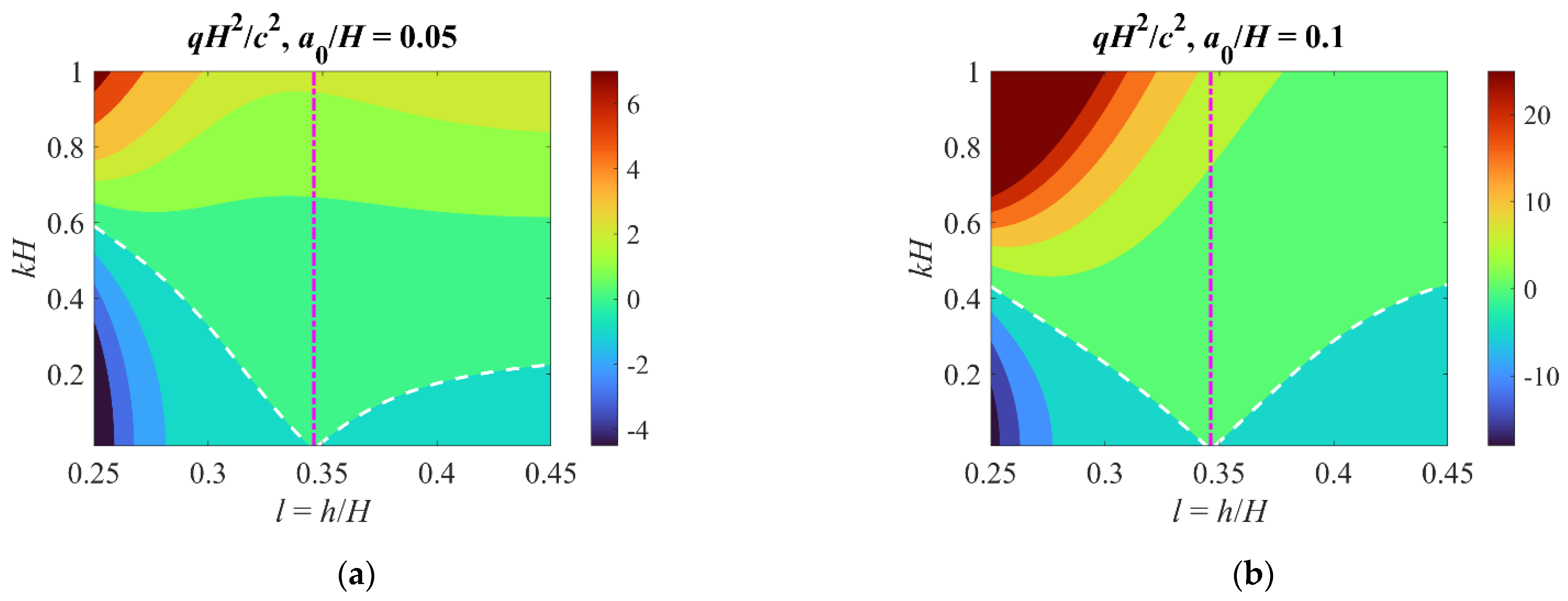
where δ = (h − hcr)/H. From expansion (55) it is clear, that in the main order; thus, a wave is stable at the critical point and at its nearest vicinity. The behavior of the nondimensional modulation instability parameter , determined by the normalized version of (54), is illustrated in Figure 3, depending on the parameter of the undisturbed medium l (which determines the dimensionless thickness of the upper and lower layers in a symmetric three-layer liquid) and the parameter , characterizing dispersion in the range of long waves , for different values of nondimensional wave amplitude: (Figure 3a) and (Figure 3b). This is fully consistent with the physical limitations of the medium (the wave amplitude should be less than the layer thicknesses) and the weakly nonlinear approximation (the wave amplitude should be significantly less than the layer thicknesses), i.e., is in the range of applicability of equation (1). The region in l is chosen to be limited taking into account the fact that equation (1) is valid only in the vicinity of the critical point l = hcr/H = 9/26 (for convenience, this critical value of the layer thickness is marked with a magenta dash-dotted line in Figure 3). The boundary of sign change for parameter (or the boundary of instability region) is shown in Figure 3 by a white dotted line, instability zone q < 0 lies under this line, it consists of two sub-regions: when l < 9/26 and when l > 9/26. Curve does not fall below than (53) when a0 increases, and curve , in opposite, rises no higher than (53) at the same time. That is, for h < hcr for more intense waves the threshold of modulation instability shifts to the region of longer waves, and the amplitude here is limited from above by the value a0*, and for h > hcr, on the contrary, the threshold of modulation instability shifts to the region of shorter waves, and the critical amplitude value a0* must be exceeded for instability to occur.
Thus, the phenomenon of modulation instability can be realized under certain combinations of environmental conditions, wavelengths and amplitudes of waves at the interfaces in a symmetrical three-layer liquid.
The upper limit of the interval of dimensionless wave numbers of the envelope (43) as a function of l (the dimensionless thickness of the upper and lower layers in a symmetrical three-layer fluid) and (dimensionless wave number of the carrier wave) is shown in Figure 4 for (Figure 4a) and (Figure 4b) in the zone of the modulation instability q < 0. Near the boundary of the instability zone q = 0, values of are small, and they increase with distance from the boundary. At smaller values of the dimensionless amplitude , values are also smaller ceteris paribus. Values of also grow when carrier wave number decreases. It is also necessary to take into account the implied ratio of carrier and envelope wavelengths k/K >> 1, with which constraint (43) must be compatible.
Maximal increment (45) as a function of l (the dimensionless thickness of the upper and lower layers in a symmetrical three-layer fluid) and (dimensionless wave number of the carrier wave) is shown in Figure 5 for (Figure 5a) and (Figure 5b) in the zone of the modulation instability q < 0. The increment grows with increasing amplitude, as well as with increasing carrier wavelength.
6. Conclusions
The conditions for the occurrence of modulation instability of weakly nonlinear quasi-monochromatic wave fields are described within the framework of the extended modified KdV equation (or (2+4)-KdV equation), which previously arose in the context of the hydrodynamics of a stratified fluid. For this purpose, an extended nonlinear Schrödinger equation of higher order associated with (2+4)-KdV was derived, which, taking into account the specifics of the considered physical context of internal waves in a three-layer liquid with symmetric stratification, where the sign of cubic nonlinearity changes, is reduced to cubic-quintic NLS equation at such a near-critical situation. Thus, it is possible to construct an approximate solution of the (2+4)-KdV equation (wave field envelope) by solving the equivalent CQ NLS equation. Furthermore, within the framework of the obtained CQ NLS equation, the instability growth rate, maximum of the increment and the boundaries of the instability interval, as well as the corresponding threshold values of the envelope amplitude are obtained analytically. It is shown that the phenomenon of modulation instability can be realized under certain combinations of environmental conditions, wavelengths and amplitudes of waves at the interfaces in a symmetrical three-layer liquid; these relationships are given analytically and examined in detail on the problem parameter planes. These results can be useful in planning numerical and laboratory experiments, as well as in explaining observed field data (within the limits of applicability of the considered approximate models).
Author Contributions
Conceptualization, O.K.; formal analysis, O.K. and A.K.; investigation, O.K., E.P. and A.K.; methodology, O.K., E.P. and A.K.; software, O.K.; supervision, A.K.; visualization, O.K.; writing—original draft, O.K., E.P. and A.K.; writing—review and editing, O.K., E.P. and A.K. All authors have read and agreed to the published version of the manuscript.
Funding
This research was funded by the State task program in the sphere of scientific activity of the Ministry of Science and Higher Education of the Russian Federation (grant No. FSWE-2023-0004).
Data Availability Statement
The data presented in this study are available on request from the corresponding author.
Acknowledgments
The authors are grateful to A.V. Slunyaev for technical assistance and discussion of the problem.
Conflicts of Interest
The authors declare no conflicts of interest.
References
- Miles, J.W. The Korteweg-de Vries equation: A historical essay. J. Fluid Mech. 1981, 106, 131–147. [Google Scholar] [CrossRef]
- Grimshaw, R. Korteweg de-Vries equation. In Nonlinear Waves in Fluids: Recent Advances and Modern Applications; Grimshaw, R., Ed.; Springer: Vienna, Austria, 2005; pp. 1–28. [Google Scholar]
- Gesztesy, F. On the Modified Korteweg-deVries Equation. In Differential Equations with Applications in Biology, Physics, and Engineering; Goldstein, J.A., Kappel, F., Schappache, W., Eds.; Marcel Dekker: New York, NY, USA, 1991; pp. 139–183. [Google Scholar]
- Wazwaz, A.M. The KdV equation. In Handbook of Differential Equations: Evolutionary Equations; Elsevier: Amsterdam, The Netherlands, 2008; Volume 4, pp. 485–568. [Google Scholar]
- Wang, X.; Zhang, J.; Wang, L. Conservation laws, periodic and rational solutions for an extended modified Korteweg-de Vries equation. Nonlinear Dyn. 2018, 92, 1507–1516. [Google Scholar] [CrossRef]
- Wadati, M. Wave propagation in nonlinear lattice. I. J. Phys. Soc. Japan 1975, 38, 673–680. [Google Scholar] [CrossRef]
- Rao, N.N.; Shukla, P.K.; Yu, M.Y. Dust-acoustic waves in dusty plasmas. Planet. Space Sci. 1990, 38, 543–546. [Google Scholar] [CrossRef]
- Helfrich, K.R.; Melville, W.K. Long nonlinear internal waves. Annu. Rev. Fluid Mech. 2006, 38, 395–425. [Google Scholar] [CrossRef]
- Kamchatnov, A.M.; Kuo, Y.-H.; Lin, T.-C.; Horng, T.-L.; Gou, S.-C.; Clift, R.; El, G.A.; Grimshaw, R.H.J. Undular bore theory for the Gardner equation. Phys. Rev. E 2012, 86, 036605. [Google Scholar] [CrossRef] [PubMed]
- Ankiewicz, A.; Bokaeeyan, M.; Chang, W. Understanding general rogue wave solutions of the Gardner equation. Rom. Rep. Phys. 2020, 72, 119. [Google Scholar]
- Pelinovsky, E.; Polukhina, O.; Slunyaev, A.; Talipova, T. Internal solitary waves. In Solitary Waves in Fluids; Chapter 4; WIT Press: Southampton, MA, USA, 2007; pp. 85–110. [Google Scholar]
- Bokaeeyan, M.; Ankiewicz, A.; Akhmediev, N. Bright and dark rogue internal waves: The Gardner equation approach. Phys. Rev. E 2019, 99, 062224. [Google Scholar] [CrossRef]
- Kurkina, O.E.; Kurkin, A.A.; Soomere, T.; Pelinovsky, E.N.; Rouvinskaya, E.A. Higher-order (2 + 4) Korteweg-de Vries-like equation for interfacial waves in a symmetric three-layer fluid. Phys. Fluids 2011, 23, 116602. [Google Scholar] [CrossRef]
- Kurkina, O.E.; Kurkin, A.A.; Ruvinskaya, E.A.; Pelinovsky, E.N.; Soomere, T. Dynamics of solitons in a nonintegrable version of the modified Korteweg-de Vries equation. JETP Lett. 2012, 95, 91–95. [Google Scholar] [CrossRef]
- Zemlyanukhin, A.I. Exact solutions of the fifth-order non-linear evolution equation. Reg. Chaotic Dyn. 1999, 4, 67–69. [Google Scholar] [CrossRef]
- Bochkarev, A.V.; Zemlyanukhin, A.I.; Mogilevich, L.I. Solitary waves in an inhomogeneous cylindrical shell interacting with an elastic medium. Acoust. Phys. 2017, 63, 148–153. [Google Scholar] [CrossRef]
- Zemlyanukhin, A.I.; Bochkarev, A.V. Exact Solutions of Cubic-Quintic Modified Korteweg-de-Vries Equation. In Nonlinear Wave Dynamics of Materials and Structures; Springer: Cham, Switzerland, 2020; Volume 122, pp. 433–445. [Google Scholar] [CrossRef]
- Gardner, C.S.; Greene, J.M.; Kruskal, M.D.; Miura, R.M. Korteweg-devries equation and generalizations. VI. methods for exact solution. Commun. Pure Appl. Math. 1974, 27, 97–133. [Google Scholar] [CrossRef]
- Miura, R.M. The Korteweg–deVries equation: A survey of results. SIAM Rev. 1976, 18, 412–459. [Google Scholar] [CrossRef]
- Ablowitz, M.J.; Segur, H. Solitons and the inverse scattering transform. In Society for Industrial and Applied Mathematics; SIAM: Philadelphia, PA, USA, 1981; pp. 1–438. [Google Scholar]
- Marchant, T.R.; Smyth, N.F. Soliton interaction for the extended Korteweg-de Vries equation. IMA J. Appl. Math. 1996, 56, 157–176. [Google Scholar] [CrossRef]
- Zabusky, N.J. Fermi–Pasta–Ulam, solitons and the fabric of nonlinear and computational science: History, synergetics, and visiometrics. Chaos 2005, 15, 15102. [Google Scholar] [CrossRef]
- Zhang, D.J.; Zhao, S.L.; Sun, Y.Y.; Zhou, J. Solutions to the modified Korteweg–de Vries equation. Rev. Math. Phys. 2014, 26, 1430006. [Google Scholar] [CrossRef]
- Osman, M.S. Multi-soliton rational solutions for some nonlinear evolution equations. Open Phys. 2016, 14, 26–36. [Google Scholar] [CrossRef]
- Arora, G.; Rani, R.; Emadifar, H. Soliton: A dispersion-less solution with existence and its types. Heliyon 2022, 8, e12122. [Google Scholar] [CrossRef]
- Dias, F.; Bridges, T. Weakly nonlinear wave packets and the nonlinear Schrödinger equation. In Nonlinear Waves in Fluids: Recent Advances and Modern Applications; Springer: Vienna, Austria, 2005; pp. 29–67. [Google Scholar]
- Fedele, R.; De Nicola, S.; Grecu, D.; Visinescu, A.; Shukla, P.K. Some mathematical aspects of the correspondence between the generalized nonlinear Schrödinger equation and the generalized Korteweg-de Vries equation. AIP Conf. Proc. 2009, 1188, 365–379. [Google Scholar]
- Pava, J.A.; Natali, F.M.A. Stability and instability of periodic travelling wave solutions for the critical Korteweg–de Vries and nonlinear Schrödinger equations. Phys. D Nonlinear Phenom. 2009, 238, 603–621. [Google Scholar] [CrossRef]
- Zakharov, V.E.; Kuznetsov, E.A. Multi-scale expansions in the theory of systems integrable by the inverse scattering transform. Phys. D 1986, 18, 455–463. [Google Scholar] [CrossRef]
- Grimshaw, R.; Pelinovsky, D.; Pelinovsky, E.; Talipova, T. Wave group dynamics in weakly nonlinear long-wave models. Phys. D Nonlinear Phenom. 2001, 159, 35–57. [Google Scholar] [CrossRef]
- Grimshaw, R.; Pelinovsky, E.; Talipova, T.; Ruderman, M.; Erdelyi, R. Short-lived large-amplitude pulses in the nonlinear long-wave model described by the modified Korteweg-de Vries equation. Stud. Appl. Math. 2005, 114, 189–210. [Google Scholar] [CrossRef]
- Chowdury, A.; Ankiewicz, A.; Akhmediev, N. Periodic and rational solutions of modified Korteweg-de Vries equation. Eur. Phys. J. D 2016, 70, 104. [Google Scholar] [CrossRef]
- Bronski, J.C.; Johnson, M.A. The modulational instability for a generalized Korteweg–de Vries equation. Arch. Ration. Mech. Anal. 2010, 197, 357–400. [Google Scholar] [CrossRef]
- Tobisch, E.; Pelinovsky, E. Constructive study of modulational instability in higher order Korteweg-de Vries equations. Fluids 2019, 4, 54. [Google Scholar] [CrossRef]
- Ostrovsky, L.A.; Potapov, A.I. Modulated Waves: Theory and Application; Johns Hopkins University Press: Baltimore, MA, USA, 2002. [Google Scholar]
- Slunyaev, A.V. A high-order nonlinear envelope equation for gravity waves in finite-depth water. J. Exp. Theor. Phys. 2005, 101, 926–941. [Google Scholar] [CrossRef]
- Birnbaum, Z.E.; Malomed, B.A. Families of spatial solitons in a two-channel waveguide with the cubic-quintic nonlinearity. Phys. D Nonlinear Phenom. 2008, 237, 3252–3262. [Google Scholar] [CrossRef]
- Abbagari, S.; Houwe, A.; Saliou, Y.; Akinyemi, L.; Rezazadeh, H.; Bouetou, T.B. Modulation instability gain and nonlinear modes generation in discrete cubic-quintic nonlinear Schrödinger equation. Phys. Lett. A 2022, 456, 128521. [Google Scholar] [CrossRef]
- Josserand, C.; Rica, S. Coalescence and droplets in the subcritical nonlinear Schrödinger equation. Phys. Rev. Lett. 1997, 78, 1215. [Google Scholar] [CrossRef]
- Luckins, E.K.; Van Gorder, R.A. Bose–Einstein condensation under the cubic–quintic Gross–Pitaevskii equation in radial domains. Ann. Phys. 2018, 388, 206–234. [Google Scholar] [CrossRef]
- Singh, H.D.; Jatav, B.S. Coherent structures and spectral shapes of kinetic Alfvén wave turbulence in solar wind at 1 AU. Res. Astron. Astrophys. 2019, 19, 093. [Google Scholar] [CrossRef]
- Djelah, G.; Ndzana, F.I.; Abdoulkary, S.; Mohamadou, A. Rogue waves dynamics of cubic–quintic nonlinear Schrödinger equation with an external linear potential through a modified Noguchi electrical transmission network. Commun. Nonlinear Sci. Numer. Simul. 2023, 126, 107479. [Google Scholar] [CrossRef]
- Chao, W. Dynamical behaviour of unbounded spatial solitons in self-defocusing media with small χ (5) self-focusing nonlinearity. Opt. Commun. 2000, 175, 239–246. [Google Scholar] [CrossRef]
- Hung, N.V.; Trippenbach, M.; Infeld, E.; Malomed, B.A. Spatial control of the competition between self-focusing and self-defocusing nonlinearities in one- and two-dimensional systems. Phys. Rev. A 2014, 90, 023841. [Google Scholar] [CrossRef]
- Onorato, M.; Waseda, T.; Toffoli, A.; Cavaleri, L.; Gramstad, O.; Janssen, P.A.E.M.; Kinoshita, T.; Monbaliu, J.; Mori, N.; Osborne, A.R.; et al. Statistical properties of directional ocean waves: The role of the modulational instability in the formation of extreme events. Phys. Rev. Lett. 2009, 102, 114502. [Google Scholar] [CrossRef] [PubMed]
- Onorato, M.; Residori, S.; Bortolozzo, U.; Montina, A.; Arecchi, F.T. Rogue waves and their generating mechanisms in different physical contexts. Phys. Rep. 2013, 528, 47–89. [Google Scholar] [CrossRef]
- Houtani, H.; Waseda, T.; Tanizawa, K. Experimental and numerical investigations of temporally and spatially periodic modulated wave trains. Phys. Fluids 2018, 30, 34101. [Google Scholar] [CrossRef]
- Houtani, H.; Sawada, H.; Waseda, T. Phase convergence and crest enhancement of modulated wave trains. Fluids 2022, 7, 275. [Google Scholar] [CrossRef]
- Klein, M.; Dudek, M.; Clauss, G.F.; Ehlers, S.; Behrendt, J.; Hoffmann, N.; Onorato, M. On the deterministic prediction of water waves. Fluids 2020, 5, 9. [Google Scholar] [CrossRef]
- Maleewong, M.; Grimshaw, R.H. Amplification of wave groups in the forced nonlinear Schrödinger equation. Fluids 2022, 7, 233. [Google Scholar] [CrossRef]
- Thorpe, S.A. On wave interactions in a stratified fluid. J. Fluid Mech. 1966, 24, 737–751. [Google Scholar] [CrossRef]
- Craik, A.D.D.; Adam, J.A. Explosive’resonant wave interactions in a three-layer fluid flow. J. Fluid Mech. 1979, 92, 15–33. [Google Scholar] [CrossRef]
- Matsuoka, C. Motion of unstable two interfaces in a three-layer fluid with a non-zero uniform current. Fluid Dyn. Res. 2021, 53, 055502. [Google Scholar] [CrossRef]
- Ha, K. Transient and Nonlinear Dynamics of Triadic Resonance for Internal Waves; Institut polytechnique de Paris: Paris, France, 2021. [Google Scholar]
- Grimshaw, R.; Pelinovsky, E.; Talipova, T. The modified Korteweg–de Vries equation in the theory of large-amplitude internal waves. Nonlin. Process. Geophys. 1997, 4, 237–350. [Google Scholar] [CrossRef]
Figure 1.
Definition sketch of a symmetric three-layer fluid.

Figure 2.
Combination of signs of coefficients , in Equation (23) on the plane in the context of interfacial waves in a three-layer fluid (a). Normalized values of on the plane (b).
Figure 2.
Combination of signs of coefficients , in Equation (23) on the plane in the context of interfacial waves in a three-layer fluid (a). Normalized values of on the plane (b).

Figure 3.
Nondimensional parameter of modulation instability (54) for (a) and (b). The white dotted line shows the sign change line , the magenta dash-dotted line shows the critical ratio of layer widths l = hcr/H = 9/26 in three-layer fluid.
Figure 3.
Nondimensional parameter of modulation instability (54) for (a) and (b). The white dotted line shows the sign change line , the magenta dash-dotted line shows the critical ratio of layer widths l = hcr/H = 9/26 in three-layer fluid.

Figure 4.
Upper limit (43) of nondimensional wavenumbers of the envelope for (a) and (b) in the zone of modulation instability q < 0.
Figure 4.
Upper limit (43) of nondimensional wavenumbers of the envelope for (a) and (b) in the zone of modulation instability q < 0.

Figure 5.
Nondimensional maximal increment (45) for (panel (a)) and (panel (b)) in the zone of the modulation instability, q < 0.
Figure 5.
Nondimensional maximal increment (45) for (panel (a)) and (panel (b)) in the zone of the modulation instability, q < 0.

Disclaimer/Publisher’s Note: The statements, opinions and data contained in all publications are solely those of the individual author(s) and contributor(s) and not of MDPI and/or the editor(s). MDPI and/or the editor(s) disclaim responsibility for any injury to people or property resulting from any ideas, methods, instructions or products referred to in the content. |
© 2024 by the authors. Licensee MDPI, Basel, Switzerland. This article is an open access article distributed under the terms and conditions of the Creative Commons Attribution (CC BY) license (https://creativecommons.org/licenses/by/4.0/).
Share and Cite
MDPI and ACS Style
Kurkina, O.; Pelinovsky, E.; Kurkin, A. Modulational Instability of Nonlinear Wave Packets within (2+4) Korteweg–de Vries Equation. Water 2024, 16, 884. https://doi.org/10.3390/w16060884
AMA Style
Kurkina O, Pelinovsky E, Kurkin A. Modulational Instability of Nonlinear Wave Packets within (2+4) Korteweg–de Vries Equation. Water. 2024; 16(6):884. https://doi.org/10.3390/w16060884
Chicago/Turabian StyleKurkina, Oksana, Efim Pelinovsky, and Andrey Kurkin. 2024. "Modulational Instability of Nonlinear Wave Packets within (2+4) Korteweg–de Vries Equation" Water 16, no. 6: 884. https://doi.org/10.3390/w16060884
Note that from the first issue of 2016, this journal uses article numbers instead of page numbers. See further details here.