Investigating First Flush Occurrence in Agro-Urban Environments in Northern Italy

Abstract

The first flush (FF) phenomenon is commonly associated with a relevant load of pollutants, raising concerns about water quality and environmental management in agro-urban areas. An FF event can potentially transport contaminated water into a receiving water body by activating combined sewer overflow (CSO) systems present in the drainage urban network. Therefore, accurately characterizing FF events is crucial for the effective management of sewer systems and for limiting environmental degradation. Given the ongoing controversy in the literature regarding the delineation of FF event occurrences, there is an unavoidable necessity for further investigations, especially experimental-based ones. This study presents the outcomes of an almost two-year field campaign focused on assessing the water quantity and quality of two combined sewer systems in Northern Italy. For this purpose, various hydro-meteorological variables, including precipitation, flow rate, temperature, and solar radiation, in addition to water quality analytics, were measured continuously to capture stormwater events. Throughout the monitoring period, sixteen stormwater events were identified and analyzed using five indices usually adopted in the literature to identify FF occurrences. The results indicate that there is a strong positive correlation between the mass first flush ratios calculated for nutrients and three factors, including maximum rainfall intensity, maximum flow rate, and antecedent dry weather period. Furthermore, rainfall duration was found to possess a strong negative correlation with the mass first flush ratios calculated for nutrients. However, for the same rainfall event, the occurrence of FF has never been unanimously confirmed by the indices examined in this study. Moreover, different macro-groups of pollutants can behave differently. Thus, it becomes apparent that relying solely on a priori analyses, without the support of data from experimental monitoring campaigns, poses a risk when designing actions for the mitigation of FF occurrences.

1. Introduction

In many regions around the world, the rapid and often poorly controlled development of urban areas is typically followed by the expansion of impervious surfaces, such as roads, parking lots, and buildings of civil and industrial use, with heavy repercussions on the quality of combined sewer overflows (CSOs) [1,2,3]. CSOs are a priority water pollution concern for municipalities served by the combined sewer systems (CSSs), since uncontrolled and unmanaged CSOs are often dispersed directly into the environment, e.g., in rural or ephemeral streams or, where feasible, in storage and infiltration ponds [4,5]. These elements are usually located in peri-urban areas, where the continuous release of untreated water can actively contribute to increasing the risk of acute and chronic pollution of soils, aquifers, and surface waters [6,7]. Specifically, CSOs can contain significant amounts of anthropogenic pollutants, such as chemicals, nutrients, microbials, and heavy metals [8,9]. Generally, the pollutant concentrations during CSO events depend on several factors, including (i) the rainfall storm severity, duration and pattern, (ii) the size of the urban catchment, (iii) the characteristics of the urban drainage system, (iv) the amount of solid or suspended solids accumulated before the storm event (i.e., during the antecedent dry period), (v) the dilution capacity of stormwater runoff during the catchment wash-off process [10,11,12].

Despite the fact that first-flush tanks (FFTs) have been largely applied as the principal countermeasure to control first flush from CSOs [13,14], i.e., the highly polluted flow at the beginning of a storm event [15], Bertrand-Krajewski et al. [16] highlighted that ‘the first flush phenomenon in stormwater discharges has been a subject for numerous and tenacious discussions, between “those who have seen it” and “those who do not believe in it”’. Nevertheless, after about twenty-five years since the work of Bertrand-Krajewski et al. [16], there is still significant controversy about first flush (FF) occurrence and definition. Concerning the definition, the controversy is related to the percentage of total pollutant load, which should be found in the first volume percentages of the event [17]. According to the literature, previous studies have considered different pollution percentages in different runoff volumes to delineate whether FF occurs or not (e.g., [10,15,16,17,18,19,20,21,22,23,24,25,26], refer to Section 2.4 for a more comprehensive explanation of the different approaches). Recently, a novel method utilizing nonparametric statistics has been proposed and employed to identify the initial and background pollutant concentrations in a catchment [27,28], but further research is needed to fully develop this methodology [17].

Notwithstanding the significant number of scientific technical papers on the FF problem in the literature, the considerations that have been made until now on the FF occurrence and definition have been derived and corroborated from a limited number of FF monitoring campaigns, especially in the Italian context [11,29,30]. Appendix A shows a brief compendium of previous experimental campaigns aimed at monitoring and collecting FF events. It reports, for each work, the number of examined basins, their dimensions, locations, the main characteristics of storm events, detected analytics, and main conclusions.

In light of previous research, this study contributes to increasing knowledge about FF occurrence by providing a glimpse into FF characteristics obtained from an extensive monitoring campaign over two real urban catchments located in the agro-urban environments of Northern Italy. During two years of monitoring campaigns, CSOs were collected by several storm events. For each storm event, flood hydrographs and pollutographs were measured and examined by applying different FF definitions to establish FF occurrences. The current study aims to (i) implement different indices to explore the occurrence of an FF event for grouped analytics (i.e., chemical oxygen demand, nutrients, and metals) and (ii) investigate whether there is a correlation between the FF occurrence and storm characteristics. The latter can be beneficial for understanding which hydro-meteorological drivers could affect the FF occurrence in favor of applying best practice management for CSSs. Furthermore, due to climate change [31], an increase in the frequency of CSO activation is expected in Northern Italy, as it has already been observed in other European regions (e.g., [32]). Hence, the results of our work can offer a perspective for understanding if alternative solutions in treating FF could be applied with respect to the traditional FFTs, in function of the characteristics of the pollution emission rate during the discharged event.

2. Materials and Methods

2.1. Study Domain

In the present study, the FF occurrence was evaluated on two different urban catchments through an extensive monitoring campaign carried out between the years 2021 and 2022. The case studies are located within an agro-urban area in the south-west of the metropolitan city of Milan, which is one of the most anthropized and industrialized areas of Northern Italy and European Union. The first urban catchment (Basin 1) coincides with the municipality of Sedriano (45°29′15″ North, 8°58′11″ East), whereas the second one (Basin 2) is represented by the municipality of Gaggiano (45°24′23″ North, 9°2′1″ East), as shown in Figure 1. Both basins can be considered very similar to each other from a hydraulic-hydrological point of view, since they have approximatively the same land use characteristics, slope, elevation, type, and density of the drainage network (

Table 1. Main physiographic characteristics of the study domains.

Basin	Characteristics	Value
Sedriano (Basin 1)	Elevation	140 m asl
	Urban drainage area	1.9 km2
	Inhabitants	4432 inh/km2
	Total length of urban drainage network	23 km
	Urban drainage network density	14.5 km/km2
	Number of conduits	686
	Mean length of the conduits	35 m
	Mean slope of the conduits	0.51%
	Mean diameter of the conduits	520 mm
Gaggiano (Basin 2)	Elevation	117 m asl
	Urban drainage area	1.2 km2
	Inhabitants	2362 inh/km2
	Total length of urban drainage network	27 km
	Urban drainage network density	22.5 km/km2
	Number of conduits	1200
	Mean length of the conduits	27 m
	Mean slope of the conduits	0.48%
	Mean diameter of the conduits	466 mm

).

The decision to deepen the knowledge on first flush in urban catchments in Northern Italy was made because only a few case studies on FF monitoring have been carried out in this area, as documented in the scientific literature [11,29]. In particular, the work of Barco et al. [11], carried out more than ten years ago on a very small urban catchment of about 12 ha, showed a clear occurrence of FF in all monitored storms, and on the basis of these results, many regional laws have used these findings to elaborate specific guidelines for the treatment of CSOs, considering FFTs as the first element to reduce the pollution load of the discharged runoff. To understand the economic impact of these decisions, in the context of the metropolitan area of Milan (approximately 1500 km² in size, 130 municipalities and 3 million inhabitants), about 200 million Euros will be invested in the next ten years by the main water manager for the design and construction of FFTs. Further field studies should therefore be carried out in this area to investigate the occurrence of FF and the need for the construction of FFTs.

Both study areas are characterized by a humid subtropical climate according to the Köppen classification system [33], although the last decade has seen an intensification of storm events (precipitation of high intensity and short duration), which have periodically put considerable pressure on the urban drainage system of both municipalities [34]. During the two monitoring years, the average annual temperature in both locations was around 7.4 °C, while the total rainfall was around 996 mm.

The urban drainage network of both sites is managed by the water and sewerage company CAP Holding. The sewerage of both urban catchments is a CSS designed to collect both wastewater and urban stormwater during rainfall events. The flow in both sewers is gravity-driven. To date, in Basin 1, the CSOs are discharged to an infiltration pond of approximately 5000 m³, located at the single outlet of the urban catchment in an open rural area close to cultivated land and irrigation canals. In Basin 2, the CSOs are discharged through four overflows within the first section of an ephemeral rural canal (called Roggia Gamberina), located in the Gaggiano municipality. The distance from the first to the last discharge point within the Roggia Gamberina is approximately 150 m. Each spillway receives runoff from four different sub-basins ranging in size from 10 to 30 ha (average 19 ha).

2.2. Hydrological and Hydraulic Data Acquisition

In Basin 1, the outlet of the drainage network was continuously monitored by an area velocity flowmeter (Kaptor^®, BM Tecnologie, Rubano, Italy) with a time resolution of 6 min. Rainfall data were collected (with a time resolution of 1 min and aggregated at 10 min) at a rain gauge located within the study area, approximately 1.5 km from the catchment outlet (Figure 1).

In Basin 2, a water level sensor (Diver^®, Eijkelkamp, Giesbeek, The Netherlands) was installed in the Roggia Gamberina, immediately after the fourth spillway, to monitor water-level fluctuations induced by the CSOs during wet periods. A stage-discharge relationship was derived using the HEC-RAS^® model to convert water level into discharge [35]. Rainfall data were collected (with a time resolution of 1 min and aggregated at 10 min) at six rain gauges located around the study area within a radius of approximately 2 km from the position of the water level sensor (Figure 1 shows the position of only one rain gauge, as the other five fall outside the boundaries of the figure). The rainfall data were then resampled using the inverse distance weighting method.

2.3. Water Quality Measurements

In both study areas, automatic water samplers (P6L Maxx^®, Maxx, Rangendingen, Germany) equipped with 24 bottles were used to collect water samples during CSO events. Each bottle had a capacity of 250 mL. In Basin 1, the automatic sampler was installed at the outlet of the urban drainage area and integrated with a float so that sampling only took place when CSOs were triggered (Figure 2a). In Basin 2, two automatic water samplers were installed in the Roggia Gamberina, approximately 10 m and 200 m downstream of the fourth spillway. However, only the first one was used for the FF assessment, as it was closer to the water level monitoring point and spillway location.

The automatic sampler was integrated with an internal software module that was able to continuously receive a signal from the water level sensor (Figure 2b). When the water level in the rural canal exceeded a pre-determined threshold, the module provided the input for sampling. The threshold was set according to the level recorded in the Roggia Gamberina before each rainfall event.

The sampling procedure consisted of three steps with different sampling time intervals. However, since the autosampler in Basin 1 was located directly at the outlet of the urban drainage network, while the autosampler in Basin 2 was installed in the rural canal (where different CSO propagation dynamics could occur), the chosen sampling time intervals differ. In Basin 1, the first eight bottles were filled every 2 min, the second eight every 5 min, and the last eight every 10 min. In Basin 2, instead, the first eight bottles were filled every 5 min, the second eight every 10 min, and the last eight every 15 min. Each bottle was completely filled with 250 mL of discharged water, and the canister was delivered to the Cap Holding labs within 4 h from collection. The bottles were grouped into pairs (the first was paired with the second, the third with the fourth, and so on) to have a sufficient water quantity for the lab analysis (i.e., 500 mL). In the case that the number of the bottles was odd, the last one was discarded. Therefore, the number of samples for each event was at most twelve. The chemical-physical parameters of the water samples, such as chemical oxygen demand (COD), TN, TP, Al, As, Cd, Cr, Fe, Mn, Ni, and Pb were evaluated based on the standard ISO protocols.

It is important to highlight that the rainfall events considered in this study (see Section 3.1) had to meet specific criteria: (i) trigger CSOs, (ii) enable the collection of at least 4 bottles, and (iii) ensure the canister reaches the Cap Holding labs within four hours from the autosampler activation. Considering the latter point, certain rain events that satisfied both CSO activations and sufficient sample bottle collections, were excluded due to delays or unavailability of technicians responsible for promptly transporting the canister to the Cap Holding labs, particularly during nighttime events.

2.4. Data Processing

2.4.1. Load-Graph Definition

FF events were studied with the load-graph, where the normalized cumulative mass (Y) of discharged pollution is depicted as a function of the normalized cumulative runoff volume (X). For instance, Saget et al. [20] investigated load-graphs of CSSs and fitted an exponential equation Y = X^a, where a is a fixed exponent called the first flush coefficient (FFC). Basically, the FFC reflects the percentage deviation of the curve from the diagonal. Based on the FFC value, Saget et al. [20] divided the load-graph into six areas by classifying the deviation from the diagonal from positive to negative and from little to strong deviation. Thus, the value of FFC was utilized in this study as a reference for detecting an FF occurrence.

As an alternative approach, the mass first flush (MFF) ratio [11,36,37,38], which can also be determined by a load-graph, was additionally introduced to address the FF occurrence in both study domains. In essence, MFF describes the fractional mass of pollutants emitted as a function of the storm’s progress. It can be also considered as the ratio of the vertical value of a point placed on the load-graph curve to the corresponding horizontal value. For example, an MFF₂₀ equal to 2.5 means that 50% of the pollutant mass is contained in the first 20% of the runoff volume. Based on the definition, MFF is equal to zero at the beginning of the storm and always equals 1 at the end of the storm. Finally, the formulation of MFF_x is presented in Equation (1) [38]:

$${\mathrm{M}\mathrm{F}\mathrm{F}}_x=\frac{\frac{{\int }_0^{t_1}C\left(t\right)Q\left(t\right)dt}{M}}{\frac{{\int }_0^{t_1}Q\left(t\right)dt}{V}}$$

(1)

where $M$ is the total pollutant mass, $V$ is the total volume of runoff, $C\left(t\right)$ is the time-dependent function of pollutant concentration, $Q\left(t\right)$ is the time-dependent function of runoff volume, and x is the index or point in the storm corresponding to the percentage of the runoff volume (i.e., ranging from 0% to 100%).

In this study, the chemical-physical parameters described in Section 2.3 were grouped into three macro analytic groups, i.e., COD, nutrients (NH4, N and P) and metals (Al, Fe, Cu, Zn) (while As, Cd, Cr, Mn, Ni and Pb were always below the limit of detection). For each group and stormwater event, a load-graph was plotted, and the FF occurrence was evaluated using different indicators, presented in Section 2.4.2.

2.4.2. Indexes of FF Occurrences

Five indices were identified from the literature and used in this study to examine the occurrences of FF (

Table 2. List of different indices used in this study to delineate first flush occurrences.

Index	Author	Condition for FF Occurrence
1	Saget et al. [20], Bertrand-Krajewski et al. [16]	FFC < 0.185
2	Lee et al. [39]	FFC < 1.0
3	Al Mamun et al. [17]	Advanced load-graph
4	Barco et al. [11], Kayhanian and Stenstorm [38]	MFFx > 1.0
5	Bertrand-Krajewski et al. [16]	${∆}_{max}>0.2$

).

According to Table 2, Saget et al. [20] and Bertrand-Krajewski et al. [16] recommend that FF occur when FFC < 0.185, indicating that at least 80% of the polluted mass is transferred within the first 30% of the runoff volume. On the other hand, Vorreiter and Hickey [19] suggest a ratio of 80% of the pollution in 25% of the runoff. According to the second index shown in Table 2, Lee et al. [39] recommend that FF be present when a positive deviation above the diagonal is observed (FFC < 1.0), which coincides with the time when the points of the load-graph are above the 45° line. Similarly, Geiger [18] recommends that FF occur when the initial slope of the load-graph curve is greater than 1. This means that, in general, the percentage of contamination should be greater than the percentage of effluent volume for any desired effluent volume.

Al Mamun et al. [17] adopted a qualitative description based on the pattern of the load-graph. A load-graph can be categorized as advanced, mixed, uniform, or lagging. According to this classification, FF occurs when the load-graph is advanced, whereas a lagging load-graph indicates no FF. In addition, a mixed load-graph consists of both an advanced and a lagging part on a single load-graph. In this type of load-graph, the existence of an FF depends on where the advanced part occurs on the load-graph. Obviously, if the leading part is at the beginning of the load-graph, it may indicate that more pollutant loads are concentrated during the early part of the storm. Furthermore, a uniform load-graph occurs when the load-graph coincides with the 45° line, indicating that there is a uniform distribution of pollutants throughout the storm.

The fourth index relies on calculating the MFF_x ratio, where x represents the percentage of runoff volume through which the mass of pollution passes. In this study, x was considered as one of these five values: 10, 20, 30, 40, and 50 [40]. According to the works of Barco et al. [11] and Kayhanian and Stenstorm [38], FF occurs when MFF_x > 1.

Lastly, the fifth index is based on the maximum difference (${∆}_{max}$) between the normalized mass and the normalized runoff volume, as shown in Equation (2):

$${∆}_{max}=X^a-X,$$

(2)

Based on the literature, FF occurs when ${∆}_{max}$ > 0.2 [16,39].

2.4.3. Method of Calculating FF Indicators

To detect the occurrence of FF, the load-graph equation (Y = X^a) was obtained from the monitored data (load and flow) by applying two different curve fitting models (i.e., a regression-based and an optimization algorithm):

In the regression-based model, as recommended by Saget et al. [20], a logarithmic function was applied to both sides of Y = X^a to make it linear. Thus, using a log transfer, the equation becomes log(Y) = a log(X) (where log is the logarithmic symbol). The value of the FFC can then simply be obtained by assuming a linear regression model between log(Y) and log(X).

A first-order optimization algorithm, called Generalized Reduced Gradient (GRG), was used to find the optimal value of FFC. In this method, the problem was treated as an optimization problem whose objective function was to minimize the root mean square error (RMSE) between the estimated normalized mass and the observed one for each group of analyses. The GRG method, embedded in MS Excel, was used to calculate the optimum value of FFC in the present study. This choice was made because the GRG method is not only easy to apply but also robust in solving water resource problems, as mentioned in previous studies [41].

After applying both curve fitting methods, two FFC values were obtained: one from the regression-based model and one from the GRG algorithm. The FFC value with the lowest RMSE was selected as the optimal FFC. In addition to Y = X^a, a polynomial relationship was also fitted to each load-graph. The MFF values were calculated using the equation (Y = X^a or the polynomial relationship) with the lowest RMSE for each group analysis and rainfall event. Finally, the calculated FFC and MFF values were used based on Table 2 to discuss the occurrence of FF events.

2.4.4. Statistical Analysis

The Pearson correlation coefficient ($R$) was used to evaluate potential correlations between discharge characteristics of overflow pollution and stormwater variables. In this study, the correlation was classified as weak ($0.10<\left|R\right|\le 0.39$), moderate ($0.4<\left|R\right|\le 0.69$), and strong ($0.7<\left|R\right|\le 1.0$), in accordance with Goodarzi et al. [42]. Furthermore, in case of no correlation, $R=0$.

Concerning stormwater variables, these include rainfall duration (min), rainfall depth (mm), maximum rainfall intensity (mm/h), CSO volume (m³), maximum flow rate (l/s), time lag (min), antecedent dry period (day), and overflow event duration (min). Among these variables, time lag was defined as the time interval between the peak of rainfall and the peak of discharge. The antecedent dry period was calculated considering three different methods: (i) scenario 1: a rainfall volume of at least 0.5 mm in 15 min [43], (ii) scenario 2: a rainfall volume of at least 10 mm in a day [44], and (iii) scenario 3: a rainfall volume of at least 1.2 mm in 30 min. Air temperature (°C) and solar radiation (W/m²) were considered in addition to the stormwater variables, as suggested by Zhang [45], since they may be important drivers for the degradation of material deposited over surfaces in dry weather periods, conditioning the nature of runoff.

3. Results

3.1. Characteristics of Storm Events, Hydrograph and Pollutograph

The characteristics of the rainfall events monitored in Basins 1 and 2 are presented in

Table 3. Characteristics of the stormwater events monitored in Basin 1.

Characteristics	Event 1	Event 2	Event 3	Event 4	Event 5	Event 6	Min	Max	Avg
Date (DD/MM/YYYY)	10 February 2021	1 May 2021	4 July 2021	8 July 2021	25 April 2022	3 November 2022	-	-	-
Rainfall duration [min]	125	60	40	55	50	750	40	750	180
Rainfall depth [mm]	8.9	7.9	14.6	12.2	16	45	7.9	45	17
Max rainfall intensity [mm/h]	9.6	25.1	56.4	31.2	48	21.6	9.6	56.4	32
CSO volume [m3]	984	1136	4754	2798	3563	4104	984	4754	2890
Max flow rate [L/s]	476	848	2175	1318	1409	792	476	2175	1170
Time lag [min]	45	35	25	35	15	200	15	200	59
Dry period [day]—scenario 1	0.04	0.05	13.91	0.85	1.91	0.03	0.03	13.91	2.8
Dry period [day]—scenario 2	1.34	18.27	26.57	3.03	110.35	0.01	0.01	110.35	26.6
Dry period [day]—scenario 3	0.17	1.87	13.90	0.83	1.91	0.01	0.01	13.90	3.1
Overflow event duration [min]	75	65	80	70	75	355	65	355	120
Air temperature [°C]	6.4	15.3	20.0	22.2	13.5	13.1	6	22	15
Solar radiation [W/m2]	0.0	51.3	298.4	158.0	0.0	0.0	0	298	85
Collected samples [bottles]	9	6	4	7	9	9	4	9	7

and

Table 4. Characteristics of the stormwater events monitored in Basin 2.

Characteristics	Event 1	Event 2	Event 3	Event 4	Event 5	Event 6	Event 7	Event 8	Event 9	Event 10	Min	Max	Avg
Date (DD/MM/YYYY)	10 February 2021	11 April 2021	30 April 2021	1 May 2021	24 May 2021	4 July 2021	8 July 2021	4 November 2021	14 November 2021	27 July 2022	-	-	-
Rainfall duration [min]	880	935	145	490	770	110	415	765	2090	480	110	2090	708
Rainfall depth [mm]	13.28	28.18	5.29	20.8	19.2	6.52	37.41	16.85	49.75	35.2	5.3	49.8	23.2
Max rainfall intensity [mm/h]	7.88	6.79	4.73	12.7	7.33	25.24	53.58	11.49	6.86	49.49	4.7	53.6	18.6
CSO volume [m3]	1386	5878	1171	4393	10,957	1947	9298	2310	22,723	6792	1171	22,723	6686
Max flow rate [l/s]	1191	1626	1466	2003	2691	2984	8050	1873	2093	4321	1191	8050	2830
Time lag [min]	35	95	75	145	160	25	25	390	1350	45	25	1350	235
Dry period [day]—scenario 1	1.93	3.35	0.15	1.75	2.06	5.61	3.78	0.06	9.46	243.17	0.06	243.17	27.13
Dry period [day]—scenario 2	1.39	58.70	16.32	1.75	11.99	26.66	3.78	0.00	9.46	242.41	0.00	242.41	37.25
Dry period [day]—scenario 3	1.97	35.71	7.81	1.75	2.07	5.60	3.78	0.09	9.46	243.24	0.09	243.24	31.15
Overflow event duration [min]	361	390	480	480	510	135	510	220	510	480	135	510	408
Air temperature [°C]	6.6	11.4	14.6	13.8	13.9	20.5	20.9	9.5	10.2	26.1	7	26	15
Solar radiation [W/m2]	6.8	48.1	115.5	29.6	77.3	294.1	53.1	0	7.8	51.7	0	294	68
Collected samples [bottles]	12	12	12	12	12	5	12	12	12	12	5	12	11

, respectively. In general, the monitored events cover a wide range of rainfall depths, intensities, and durations.

Specifically, the rainfall depth ranged from 5.3 mm to 49.8 mm, while the rainfall duration ranged from 40 min to 2090 min. Based on Table 3 and Table 4, the rainfall events produced CSO volumes ranging from 984 m³ to 22,723 m³, with a lag time of 15 to 1350 min during the field campaign. Furthermore, Table 3 and Table 4 show that the antecedent dry periods obtained by the first and third scenarios are closer for most storm events, while the second scenario produced different dry period values for a few events.

Moreover, Event 6 in Basin 1 (Table 3) and Event 8 in Basin 2 (Table 4) exhibit notably low values of antecedent dry periods. Despite this, we decided to incorporate these events into our analysis to assess the selected indices (Table 2) concerning CSO releases in the absence of a relevant antecedent dry period.

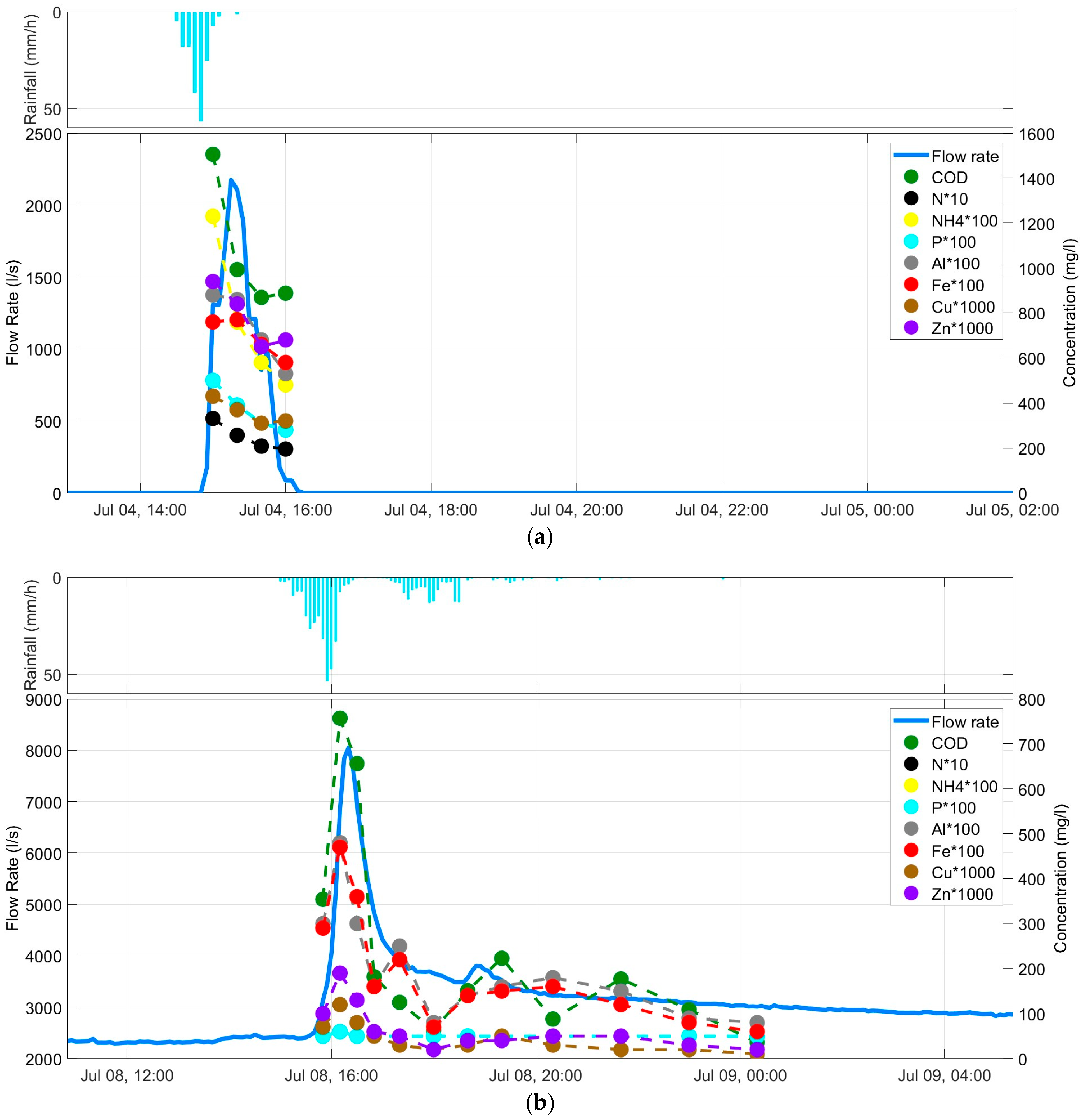
Figure 3a,b show an example of what happened during a typical CSO event in Basins 1 and 2 through a visual inspection of the hyetograph, hydrograph, and pollutograph elements (the latter subdivided among different chemical parameters), respectively. All CSOs had relatively sharp hydrographs, as expected for urban systems. In general, the CSOs were triggered after a time lag, which depended on the catchment, the urban drainage network, the rainfall characteristics, and the antecedent conditions before the rainfall. The hydrograph pattern gradually increases to a maximum flow rate and then decreases. Traditional first-flush paradigms result in decreasing contaminant concentrations along the hydrograph due to dilution and/or source mass depletion across the catchments [46]. This was observed in all events in both Basin 1 and 2.

3.2. Identification of First Flush Occurrence in Overflow Events

3.2.1. First Flush Occurrence in Basin 1

Variations in normalized mass for each group of water quality parameters (COD, metals, and nutrients) for six rainfall events that occurred in Basin 1 are shown in Figure 4.

As can be seen, most of the points with normalized runoff volumes greater than 0.2 are below the 45° line in the load-graphs, while a few points are on or above the 45° line. Only the nutrient (and partly COD) pattern in Event 4 (8 July 2021) showed a strong deviation below the diagonal, probably due to a complete washing action of the basin surface after the preceding event, four days earlier (i.e., Event 3 on 4 July 2021). In addition, Figure 4 highlights that the transfer of pollutants of different quality groups follows quite similar patterns in Basin 1.

Although Figure 4 visually indicates that FF only occurred during a few rainfall events, it is still necessary to use mathematical calculations to identify the actual presence of FF. Therefore, the five FF indices (described in Section 2.4.2) were used to delineate the occurrence of FF events for each analysis group in Basin 1, while the corresponding results are presented in

Table 5. FF occurrence indices for stormwater events that occurred from February 2021 to November 2022 in Basin 1.

Event	Analytic	FFC	MFF20	${∆}_{\mathit{m}\mathit{a}\mathit{x}}$	Index 1	Index 2	Index 3	Index 4	Index 5
1	COD	1.612	0.72	−0.02	No	No	Lagging	No	No
	Nutrients	1.484	0.72	−0.02	No	No	Lagging	No	No
	Metals	1.477	0.85	0.00	No	No	Lagging	No	No
2	COD	0.967	1.42	0.08	No	Yes	Mixed	Yes	No
	Nutrients	1.177	1.25	0.05	No	No	Mixed	Yes	No
	Metals	1.122	1.27	0.05	No	No	Mixed	Yes	No
3	COD	2.156	0.14	−0.01	No	No	Lagging	No	No
	Nutrients	1.954	0.28	−0.01	No	No	Lagging	No	No
	Metals	2.013	0.24	−0.01	No	No	Lagging	No	No
4	COD	1.491	0.80	−0.01	No	No	Lagging	No	No
	Nutrients	1.837	0.89	0.01	No	No	Lagging	No	No
	Metals	1.266	0.96	0.01	No	No	Lagging	No	No
5	COD	0.932	1.34	0.07	No	Yes	Mixed	Yes	No
	Nutrients	1.034	1.18	0.04	No	No	Mixed	Yes	No
	Metals	1.018	1.20	0.04	No	No	Mixed	Yes	No
6	COD	0.920	1.23	0.05	No	Yes	Mixed	Yes	No
	Nutrients	0.868	1.37	0.08	No	Yes	Mixed	Yes	No
	Metals	0.803	1.46	0.10	No	Yes	Mixed	Yes	No

.

In general, all five indices give a similar result for the occurrence of FF events. However, there are nine cases where the FF indices disagree on whether an FF event has occurred. These cases are presented below:

(1) Event 2 for COD: The calculated FFC ($a$ = 0.967) is greater than 0.185 and less than 1, while ${∆}_{max}$ is less than 0.2. Thus, based on the first and fifth indices, it indicates no FF, while the second index shows that the FF occurred. The latter agrees with the result of the fourth index, since MFF₂₀ (i.e., 1.42) is higher than 1 in this case. The third index gives a qualitative result, which is a mixed type of load-graph.

(2) Event 2 for nutrients: Based on the FFC value (i.e., 1.177), the first and second indices indicate no FF, whereas MFF₂₀ (i.e., 1.25) indicates that an FF event occurred. The fifth index also indicates no FF, as ${∆}_{max}$ is less than 0.2 for all grouped analyses.

(3) Event 2 for metals: the same disagreement as for event 2 for nutrients was obtained for this case.

(4) Event 5 for COD: According to Table 5, the calculated FFC (i.e., 0.932) is higher than 0.185 but lower than 1.0, resulting in No and Yes for the occurrence of FF based on the first and second indices, respectively. Furthermore, the fourth index indicates the occurrence of an FF because MFF₂₀ (i.e., 1.34) is higher than 1.0.

(5) Event 5 for nutrients: the first, second and fifth indices do not indicate an FF because FFC (i.e., 1.034) is greater than 1 and ${∆}_{max}$ = 0.04 < 0.2, while the fourth index does indicate an FF because MFF₂₀ (i.e., 1.18) is greater than 1.0.

(6) Event 5 for metals: there is a similar disagreement as for event 5 for nutrients.

(7–9) Event 6 for COD, nutrients, and metals: in all three cases, the FFC values are greater than 0.185 but less than 1.0, resulting in neither FF based on the first index nor FF occurrence based on the second index.

Consistent with the second index, the fourth index also shows that FF occurred in the three cases, since MFF₂₀ is greater than 1.0, as shown in Table 5. Finally, the fifth index agrees with the results of the first index, as the corresponding ${∆}_{max}$ values are lower than 0.2.

In addition to examining the occurrence of FF for each pollutant macro group, it is useful to have a look at the average pollutant transfer during each rainfall event. In this regard,

Table 6. Variation of MFF_x and ${∆}_{max}$ averaged for stormwater events that occurred from February 2021 to November 2022 in Basin 1.

Events	MFF10	MFF20	MFF30	MFF40	MFF50	${∆}_{\mathit{m}\mathit{a}\mathit{x}}$
Event 1	0.83	0.76	0.72	0.69	0.69	−0.01
Event 2	1.50	1.31	1.16	1.05	0.96	0.06
Event 3	0.12	0.22	0.32	0.41	0.51	−0.01
Event 4	1.00	0.88	0.79	0.73	0.70	0.00
Event 5	1.37	1.24	1.13	1.04	0.98	0.05
Event 6	1.47	1.35	1.25	1.16	1.09	0.07
Average	1.05	0.96	0.89	0.85	0.82	0.03

shows the average MFF_x and ${∆}_{max}$ values for each event and all events in Basin 1. For example, the MFF₁₀ and ${∆}_{max}$ values for Event 1 were obtained by averaging the MFF₁₀ and ${∆}_{max}$ values obtained for each analytic group, respectively. According to Table 6, no FF is observed for events 1, 3 and 4, regardless of which MFF_x or ${∆}_{max}$ is considered, as all MFF_x are less than 1.0 and ${∆}_{max}$ is less than 0.2 for the corresponding events. For events 2 and 5, MFF_x when x = 10, 20, 30, and 40, as well as ${∆}_{max}$ values, show that FF occurred during these two events, whereas MFF₅₀ indicates that there was no FF. On the other hand, all MFF_x and ${∆}_{max}$ values calculated for event 6 show that FF occurred. Based on Table 6, the MFF₁₀ and ${∆}_{max}$ values averaged for all six events show that Basin 1 is susceptible to experiencing FF events, whereas MFF₂₀, MFF₃₀, MFF₄₀, and MFF₅₀ show an opposite trend regarding the occurrence of FF in Basin 1. Therefore, for all cases observed during the field campaign in Basin 1, MFF₂₀, MFF₃₀, and MFF₄₀ gave the same results regarding the occurrence of FF.

3.2.2. First Flush Occurrence in Basin 2

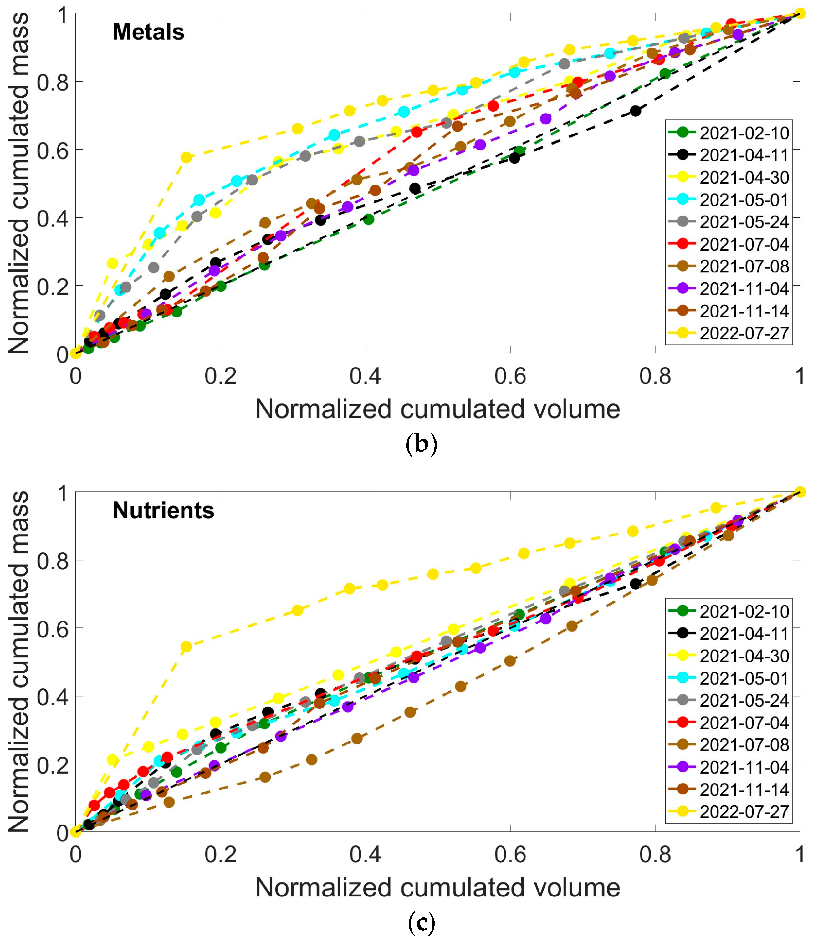
Figure 5 shows the variations of the normalized cumulative mass for each group of pollutants in relation to the normalized cumulative volume in Basin 2. As can be seen, in contrast to Figure 4, most of the points measured during stormwater events are above the 45° line. More specifically, the normalized mass for COD and metals is higher for most of the events observed in Basin 2. Furthermore, Figure 5 visually demonstrates that the occurrence of FF in Basin 2 is probable, and consequently, different indices were used to quantify the occurrence of FF.

Table 7. FF occurrence indices for stormwater events that occurred from February 2021 to July 2022 in Basin 2.

Event	Analytic	FFC	MFF20	${∆}_{\mathit{m}\mathit{a}\mathit{x}}$	Index 1	Index 2	Index 3	Index 4	Index 5
1	COD	1.118	0.80	0.00	No	No	Lagging	No	No
	Nutrients	0.883	1.23	0.05	No	Yes	Advanced	Yes	No
	Metals	1.024	0.96	0.00	No	No	Uniform	No	No
2	COD	0.826	1.58	0.12	No	Yes	Mixed	Yes	No
	Nutrients	0.844	1.43	0.09	No	Yes	Mixed	Yes	No
	Metals	0.899	1.34	0.07	No	Yes	Mixed	Yes	No
3	COD	0.423	2.53	0.31	No	Yes	Advanced	Yes	Yes
	Nutrients	0.698	1.62	0.13	No	Yes	Advanced	Yes	No
	Metals	0.498	2.24	0.25	No	Yes	Advanced	Yes	Yes
4	COD	0.406	2.60	0.32	No	Yes	Advanced	Yes	Yes
	Nutrients	0.884	1.33	0.07	No	Yes	Advanced	Yes	No
	Metals	0.465	2.36	0.31	No	Yes	Advanced	Yes	Yes
5	COD	0.494	2.28	0.31	No	Yes	Advanced	Yes	Yes
	Nutrients	0.844	1.29	0.06	No	Yes	Advanced	Yes	No
	Metals	0.538	2.13	0.26	No	Yes	Advanced	Yes	Yes
6	COD	0.614	1.79	0.22	No	Yes	Advanced	Yes	Yes
	Nutrients	0.643	1.74	0.12	No	Yes	Advanced	Yes	No
	Metals	0.641	1.72	0.14	No	Yes	Advanced	Yes	No
7	COD	0.576	1.98	0.20	No	Yes	Advanced	Yes	No
	Nutrients	1.342	0.59	0.00	No	No	Lagging	No	No
	Metals	0.726	1.55	0.12	No	Yes	Advanced	Yes	No
8	COD	0.636	1.63	0.19	No	Yes	Mixed	Yes	No
	Nutrients	1.016	0.99	0.01	No	No	Mixed	No	No
	Metals	0.836	1.25	0.21	No	Yes	Advanced	Yes	Yes
9	COD	0.920	1.07	0.05	No	Yes	Mixed	Yes	No
	Nutrients	0.952	1.05	0.03	No	Yes	Mixed	Yes	No
	Metals	0.850	1.15	0.10	No	Yes	Mixed	Yes	No
10	COD	0.301	3.08	0.42	No	Yes	Advanced	Yes	Yes
	Nutrients	0.363	2.79	0.36	No	Yes	Advanced	Yes	Yes
	Metals	0.331	2.93	0.39	No	Yes	Advanced	Yes	Yes

summarizes the results of each index for detecting the occurrence of FF in Basin 2 for each type of grouped pollutant. As can be seen, there is an inconsistency in many cases. Specifically, the first and fifth indices did not detect FF in 26 and 15 cases, respectively, where FF was detected using the second and fourth indices. Therefore, the second and fourth indices have quite the same threshold for the occurrence of FF, while the first and fifth indices yield quite the same results. However, the first one has a very limited threshold, which is the reason why it did not detect FF for all the cases listed in Table 7, whereas the second and fourth indices confirm the presence of FF in 26 cases. The third index, which is qualitative, agrees with the second and fourth indices in 22 out of 30 cases. In addition, FF did not occur at least once for each type of water quality analysis. Furthermore, the results of the second, third and fourth indices show that Basin 2 is susceptible to FF, as they reveal the occurrence of FF in many of the ten events during the field campaign.

Table 8. Variation of MFF_x and ${∆}_{max}$ averaged for stormwater events that occurred from February 2021 to July 2022 in Basin 2.

Events	MFF10	MFF20	MFF30	MFF40	MFF50	${∆}_{\mathit{m}\mathit{a}\mathit{x}}$
Event 1	1.00	1.00	1.00	1.00	1.00	0.02
Event 2	1.65	1.45	1.28	1.15	1.04	0.09
Event 3	2.98	2.13	1.76	1.53	1.38	0.23
Event 4	2.70	2.10	1.77	1.54	1.37	0.23
Event 5	2.14	1.90	1.70	1.53	1.38	0.21
Event 6	1.65	1.54	1.44	1.36	1.28	0.16
Event 7	1.68	1.37	1.24	1.16	1.11	0.11
Event 8	1.32	1.29	1.26	1.23	1.20	0.13
Event 9	1.07	1.09	1.10	1.11	1.11	0.06
Event 10	4.67	2.93	2.24	1.84	1.59	0.39
Average	2.09	1.68	1.48	1.34	1.25	0.16

presents MFF_x and ${∆}_{max}$ values averaged for the ten stormwater events monitored in Basin 2. According to the results of Event 1 in Table 7, FF occurs for nutrients and not for COD and metals (based on the second and fourth indexes), while Table 8 shows no FF, based on averaged MFF_x (x = 10, 20, 30, 40, and 50) and ${∆}_{max}$. This shows that FF can occur based on specific groups of pollutants, while it may not be detected when all analyses are considered. Furthermore, in events 2, 6, 7, 8 and 9, FF occurred based on averaged MFF_x (x = 10, 20, 30, 40, and 50), whereas ${∆}_{max}$ confirms no FF for the same events. This discrepancy between MFF_x (x = 10, 20, 30, 40, and 50) and ${∆}_{max}$ for Basin 2 shows that the latter is a more restrictive limit than the former. Furthermore, both the averaged MFF_x (x = 10, 20, 30, 40, and 50) and ${∆}_{max}$ resulted in the occurrence of FF for events 3, 4, 5, and 10. In addition, Table 8 shows that FF is observed for all events based on averaged MFF_x (x = 10, 20, 30, 40, and 50), whereas the value of ${∆}_{max}$ averaged for all 10 events in Basin 2 is less than 0.2, indicating no FF. Thus, there is another inconsistency between MFF_x (x = 10, 20, 30, 40, and 50) and ${∆}_{max}$ regarding the occurrence of FF when considering an average value for all 10 events.

3.3. Insights about First Flush Occurrence Drivers

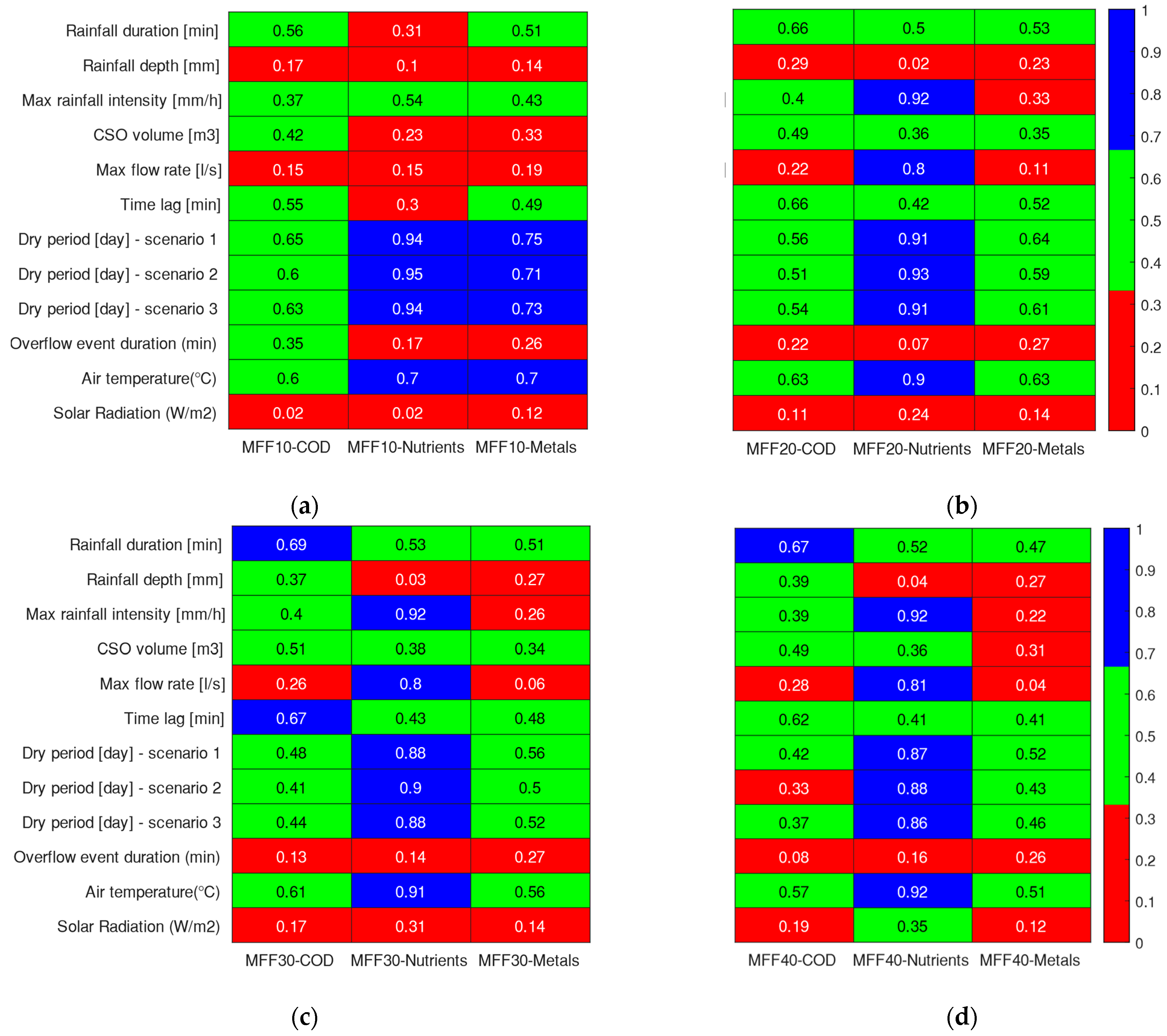
As mentioned in the introduction, the environmental factors that can influence the occurrence of FF are typically the type of pollutant, the size of the catchment, the impervious area contributing to the runoff, the characteristics of the runoff (i.e., maximum discharge), the characteristics of the rainfall event (rainfall duration, maximum rainfall intensity, and antecedent dry period), and meteorological parameters (i.e., air temperature and solar radiation). To investigate the causes of FF events, the Pearson correlation coefficient ($R$) between MFF_x (x = 10, 20, 30, 40 and 50) and ${∆}_{max}$ was calculated for the events identified as FF. Since most of the events in Basin 1 are associated with MFF_x less than 1.0 and ${∆}_{max}$ less than 0.2, no events from Basin 1 were used to calculate R. Figure 6 illustrates the $R$ obtained for MFF_x (x = 10, 20, 30, 40, and 50) and ${∆}_{max}$, considering only the data from Basin 2.

Before delving into the specific outcomes of the correlation matrix, it is important to emphasize that some environmental variables could be, in turn, correlated with each other. For instance, the climate in Northern Italy, marked by wet winters and dry summers, suggests a potential correlation between the air temperature and the antecedent dry period. Likewise, and more obviously due to the hydrological process, there exists a correlation between, e.g., the peak flow rate and the maximum rainfall intensity.

As shown in Figure 6a, there is a positive correlation between the antecedent dry period ($0.60\le R\le 0.95$) and air temperature ($0.6\le R\le 0.7$) and MFF₁₀ obtained for all grouped pollutants, as their correlation coefficients are higher than 0.5. More specifically, there is a strong correlation ($0.94\le R\le 0.95$) between the MFF₁₀ calculated for nutrients and the antecedent dry period, regardless of the scenario based on which it was calculated. Furthermore, Figure 6a shows that the MFF₁₀ calculated for nutrients is also correlated ($R=0.54$) with the maximum rainfall intensity.

According to Figure 6b, MFF₂₀ for nutrients has a strong positive correlation with maximum rainfall intensity ($R=0.92$), maximum discharge ($R=0.8$), antecedent dry period ($0.91\le R\le 0.93$), and air temperature ($R=0.9$). In addition, the calculated $R$ values show that MFF₂₀ for COD and metals, such as MFF₁₀, has a positive correlation with the antecedent dry period and air temperature. Similar positive correlations can be observed between MFF₃₀, MFF₄₀, and MFF₅₀ calculated for nutrients and maximum rainfall intensity ($0.9\le R\le 0.92$), maximum discharge ($0.8\le R\le 0.82$), antecedent dry period ($0.84\le R\le 0.90$) and air temperature ($0.91\le R\le 0.92$). In addition, MFF₃₀ has a moderate positive correlation with the antecedent dry period ($0.41\le R\le 0.48$ for COD and $0.50\le R\le 0.56$ for metals) and air temperature ($R=0.61$ for COD and $R=56$ for metals). MFF₄₀ also has a moderate positive correlation with air temperature ($R=0.57$ for COD and $R=51$ for metals), while a moderate positive correlation was found between MFF₅₀ and air temperature ($R=0.53$ for COD).

Comparing the correlation coefficients between MFF_x and the antecedent dry period, increasing x from 10 to 50 reduces the $R$ calculated between MFF_x for each group of pollutants and the antecedent dry period, regardless of the scenario used to calculate the antecedent dry period. MFF₂₀, MFF₃₀, MFF₄₀, and MFF₅₀ for nutrients have a strong positive correlation ($0.8\le R\le 0.82$), with maximum flow rate, while $R$ between MFF₁₀ for nutrients and maximum flow rate is 0.15. A similar pattern can be seen for maximum rainfall intensity. More precisely, MFF₂₀, MFF₃₀, MFF₄₀, and MFF₅₀ for nutrients have a strong positive correlation ($0.9\le R\le 0.92$), with maximum rainfall intensity, whereas a moderate correlation ($R=0.54$) was obtained between MFF₁₀ for nutrients and maximum rainfall intensity. Since Figure 6 presents correlation matrices with absolute values for comparison purposes, negative correlations, such as the one between MFF_x for each analysis and rainfall duration ($-0.69\le R\le -0.31$), are shown with absolute values.

Figure 6f shows that ${∆}_{max}$ is strongly correlated with the antecedent dry period ($0.73\le R\le 0.75$ for COD and $0.83\le R\le 0.84$ for metals). Furthermore, ${∆}_{max}$ for metals is strongly correlated with rainfall depth ($R=0.8$), maximum rainfall intensity ($R=0.85$), maximum flow rate ($R=0.81$) and air temperature ($R=0.91$), whereas it has a moderate correlation with the duration of the overflow event ($R=0.57$). On the other hand, a correlation between ${∆}_{max}$ for nutrients and other parameters could not be calculated, as there was only one event where an FF was observed based on ${∆}_{max}$.

4. Discussion

In Basin 1, six CSO events were monitored from February 2021 to July 2022, and FF was observed in three out of six cases based on MFF₂₀, while no FF was identified with respect to ${∆}_{max}$, as shown in Table 6. In the same period, ten CSO events were monitored in Basin 2, and FF was observed much more often (nine out of ten events based on MFF₂₀) than in Basin 1. In general, most of the load-graph plots obtained for the events that occurred in Basin 1 have a small deviation below the diagonal, while a few of them have a small deviation above the diagonal, as shown in Figure 4. On the contrary, most of the stormwater events in Basin 2 have load-graph plots with a significant deviation above the diagonal, as shown in Figure 5. This finding seems to be consistent with the results of previous studies, regarding the presence of FF in small basins compared to larger ones [11,17]. Moreover, it is noteworthy that Event 6 in Basin 1 and Event 8 in Basin 2, despite being characterized by the absence of an antecedent dry period, still exhibit FF (considering MFF₂₀). Hence, the antecedent dry period seems not to be decisive in determining whether a rainfall event exhibits an FF or not, but rather in amplifying its effects.

Examining the five indices utilized to discern the occurrence of an FF, a 50% consensus was observed for Basin 1, while a mere 10% agreement was noted for Basin 2. It is also interesting to note how the agreement between all indices occurs only in indicating that an FF has not occurred. Indeed, index 1 (i.e., FFC < 0.185 [16,20]) never indicated the presence of an FF for any rainfall event or water quality analytics (COD, nutrients, and metals). This outcome aligns with prior studies, indicating that index 1 is notably restrictive (e.g., Lee et al. [47] found that only 1% of the events satisfy this condition). Considering the other indices, index 5 (i.e., ${∆}_{max}$ > 0.2 [16]) is the second most restrictive in indicating the presence of an FF, followed by index 3 (i.e., advanced load-graph [17]), and, finally, by indices 2 (i.e., FFC < 1 [39]) and 4 (i.e., MFF₂₀ > 1 [11,38]). The latter two indices appear to be almost equivalent giving similar results.

Considering the macro water quality analytic groups, the FF shows a general tendency wherein its relative strength follows the order COD ≳ metals > nutrients. This trend is in accordance with other case studies present in the literature (e.g., [11,26,47]).

The correlation matrices shown in Figure 6 indicate that MFF_x (when x = 20%, 30%, 40%, and 50%) generally have a good correlation with the following environmental factors, i.e., rainfall duration, rainfall intensity, antecedent dry period, and air temperature. More specifically, a negative correlation was found with rainfall duration and a positive correlation with rainfall intensity. The increased energy from heavy rainfall may result in the transport of a substantial amount of material deposited on surfaces during dry days and the resuspension of settled particulate matter. Regarding the correlation between air temperature and the occurrence of FF, the results (i.e., positive correlations, shown in Figure 6) are consistent with those found by Zhang [45]. Indeed, he found that an increase in air temperature leads to an increase in nutrient solubility, indicating that air temperature is associated with nutrient release from the watershed [45].

Table 9. Comparison of different studies regarding the reported correlation between the occurrence of FF and hydrological and hydraulic variables. The “-” symbol indicates that the variable has not been analyzed.

Author		Maximum Rainfall Intensity	Maximum Flow Rate	Rainfall Duration	Antecedent Dry Weather Period
Gupta and Saul [10]		Yes	Yes	Yes	Yes
Bertrand-Krajewski et al. [16]		No	No	No	No
Lee and Bang [49]		Slight correlation	-	-	No
Lee et al. [39]		-	-	-	No
Athanasiadis et al. [48]		No	No	No	No
Our study (based on MFFx)	COD	Moderate ($0.37\le R\le 0.40$)	Weak ($0.15\le R\le 0.28$)	Negative correlation ($-0.69\le R\le -0.31$)	Weak and moderate ($0.26\le R\le 0.65$)
	Nutrients	Moderate and strong ($0.54\le R\le 0.92$)	Weak and strong ($0.15\le R\le 0.82$)		Strong ($0.84\le R\le 0.95$)
	Metals	Weak and moderate ($0.20\le R\le 0.43$)	Weak ($0.03\le R\le 0.19$)		Moderate ($0.38\le R\le 0.75$)

compares the outcome of different studies regarding the correlation between the FF occurrence and various factors that may trigger the occurrence of FF events. As shown, Gupta and Saul [10] reported a correlation between the FF occurrence and the maximum rainfall intensity, maximum flow rate, rainfall duration, and antecedent dry weather period. However, Bertrand-Krajewski et al. [16] and Athanasiadis et al. [48] did not find such correlations. Furthermore, Lee and Bang [49] and Lee et al. [39] concluded that there was no correlation between FF occurrence and antecedent dry periods. However, they reported a slight correlation between the maximum rainfall intensity and the occurrence of the FF phenomenon. In addition, this study explores the existence of correlations between FF occurrences and other parameters involved, based on each group of pollutants, as illustrated in Figure 6. Indeed, the type of pollutant may have an impact on MFF_x, as indicated by both previous studies [30,49] and our results, presented in Table 5, Table 6, Table 7 and Table 8. According to Barone et al. [29], the occurrence of FF for nutrients has a strong correlation with the antecedent dry period. Furthermore, Table 9 indicates that the occurrence of FF events has a negative correlation with rainfall duration, regardless of the type of pollutant. Moreover, the correlation between the maximum flow rate and maximum rainfall intensity with the occurrence of FF for COD and metals is weak to moderate, as indicated by the MFF_x values shown in Figure 6. Similarly, the correlation between the antecedent dry period with the occurrence of FF for COD and metals is also weak to moderate.

Considering the limitations of this study, the primary challenge lies in the fact that, despite the nearly two-year duration of the measurement campaign, only sixteen rainfall events were accurately sampled. Unfortunately, some measurements were lost due to nocturnal occurrences, making it impractical for the personnel to promptly transport samples to the laboratory for chemical analysis. Another shortcoming of our analysis is the oversight of the bacterial load released by the CSOs [50]. Moving forward, the information gathered with this experimental campaign will be pivotal for investigating, from an engineering standpoint, the most effective solutions for managing the flows from CSOs that present a not-so-pronounced FF. In such instances, the pollutant load is not mainly concentrated in the initial phase of the overflow, thereby making the management of these waters more challenging and the use of traditional FFTs questionable [4,13].

5. Conclusions

This study reports the results of an almost two-year field campaign conducted in two agro-urban basins located in Northern Italy, focusing on the occurrence of FF. Overall, sixteen combined sewer overflow events were monitored and studied. The results appear consistent with that part of the literature that considers the presence of the FF somewhat contentious. The presence of FF has never been confirmed contemporaneously by all the indices used in this work, neither in Basin 1 nor in Basin 2. Furthermore, there are contrasting results between the indices calculated for the same rainfall events across the different macro-groups of pollutants considered in this study (i.e., COD, nutrients, and metals). This highlights how the occurrence of FF correlates with the type of pollutant. The correlations between FF occurrence and hydro-meteorological variables also reflect the variability of results reported in the literature, again highlighting different levels of correlation between the macro group of pollutants and the same hydro-meteorological variable.

In conclusion, the results suggest that the occurrence of FF in real-case sites could not be defined a priori but should be carefully evaluated through accurate field measurement campaigns. Only based on these results could effective prevention strategies be found for the management and removal of FF [5,12,51]. This is especially true in the context of climate change adaptation, where innovative strategies (such as nature-based solutions and urban greening) show a much higher benefit/cost ratio compared to traditional gray solutions [52].

References

- Ercolani, G.; Chiaradia, E.A.; Gandolfi, C.; Castelli, F.; Masseroni, D. Evaluating performances of green roofs for stormwater runoff mitigation in a high flood risk urban catchment. J. Hydrol. 2018, 566, 830–845. [Google Scholar] [CrossRef]
- Quaranta, E.; Fuchs, S.; Liefting, H.J.; Schellart, A.; Pistocchi, A. A hydrological model to estimate pollution from combined sewer overflows at the regional scale: Application to Europe. J. Hydrol. Reg. Stud. 2022, 41, 101080. [Google Scholar] [CrossRef]
- ISPRA. Consumo di Suolo, Dinamiche Territoriali e Servizi Ecosistemici. Edizione 2023; Report SNPA 37/23; ISPRA: Rome, Italy, 2023. (In Italian) [Google Scholar]
- Masseroni, D.; Ercolani, G.; Chiaradia, E.A.; Maglionico, M.; Toscano, A.; Gandolfi, C.; Bischetti, G.B. Exploring the performances of a new integrated approach of grey, green and blue infrastructures for combined sewer overflows remediation in high-density urban areas. J. Agric. Eng. 2018, 49, 233–241. [Google Scholar] [CrossRef]
- Rizzo, A.; Tondera, K.; Pálfy, T.G.; Dittmer, U.; Meyer, D.; Schreiber, C.; Zacharias, N.; Ruppelt, J.P.; Esser, D.; Molle, P.; et al. Constructed wetlands for combined sewer overflow treatment: A state-of-the-art review. Sci. Total Environ. 2020, 727, 138618. [Google Scholar] [CrossRef] [PubMed]
- Ferrario, C.; Tesauro, M.; Consonni, M.; Tanzi, E.; Galli, A.; Peruzzi, C.; Beltrame, L.; Gandolfi, C.; Masseroni, D. Impact of combined sewer overflows on water quality of rural canals in agro-urban environments. In Proceedings of the 18th Annual Meeting of the Asia Oceania Geosciences Society (AOGS 2021), Singapore, 1–6 August 2021. [Google Scholar]
- Masood, A.; Niazkar, M.; Zakwan, M.; Piraei, R. A Machine Learning-Based Framework for Water Quality Index Estimation in the Southern Bug River. Water 2023, 15, 3543. [Google Scholar] [CrossRef]
- Gasperi, J.; Zgheib, S.; Cladière, M.; Rocher, V.; Moilleron, R.; Chebbo, G. Priority pollutants in urban stormwater: Part 2—Case of combined sewers. Water Res. 2012, 46, 6693–6703. [Google Scholar] [CrossRef] [PubMed]
- Launay, M.A.; Dittmer, U.; Steinmetz, H. Organic micropollutants discharged by combined sewer overflows–characterisation of pollutant sources and stormwater-related processes. Water Res. 2016, 104, 82–92. [Google Scholar] [CrossRef] [PubMed]
- Gupta, K.; Saul, A.J. Specific relationships for the first flush load in combined sewer flows. Water Res. 1996, 30, 1244–1252. [Google Scholar] [CrossRef]
- Barco, J.; Papiri, S.; Stenstrom, M.K. First flush in a combined sewer system. Chemosphere 2008, 71, 827–833. [Google Scholar] [CrossRef] [PubMed]
- Gao, Z.; Zhang, Q.; Li, J.; Wang, Y.; Dzakpasu, M.; Wang, X.C. First flush stormwater pollution in urban catchments: A review of its characterization and quantification towards optimization of control measures. J. Environ. Manag. 2023, 340, 117976. [Google Scholar] [CrossRef]
- Albizzati Mantegazza, S.; Gallina, A.; Mambretti, S.; Lewis, C. Designing CSO storage tanks in Italy: A comparison between normative criteria and dynamic modelling methods. Urban Water J. 2010, 7, 211–216. [Google Scholar] [CrossRef]
- Todeschini, S.; Papiri, S.; Ciaponi, C. Performance of stormwater detention tanks for urban drainage systems in northern Italy. J. Environ. Manag. 2012, 101, 33–45. [Google Scholar] [CrossRef]
- Thornton, R.C.; Saul, A.J. Temporal variation of pollutants in two combined sewer systems. In Proceedings of the 4th International Conference on Urban Storm Drainage, Lausanne, Switzerland, 31 August–4 September 1987; pp. 51–52. [Google Scholar]
- Bertrand-Krajewski, J.L.; Chebbo, G.; Saget, A. Distribution of pollutant mass vs volume in stormwater discharges and the first flush phenomenon. Water Res. 1998, 32, 2341–2356. [Google Scholar] [CrossRef]
- Al Mamun, A.; Shams, S.; Nuruzzaman, M. Review on uncertainty of the first-flush phenomenon in diffuse pollution control. Appl. Water Sci. 2020, 10, 53. [Google Scholar] [CrossRef]
- Geiger, W. Flushing effects in combined sewer systems. In Proceedings of the 4th International Conference on Urban Storm Drainage, Lausanne, Switzerland, 31 August–4 September 1987; pp. 40–46. [Google Scholar]
- Vorreiter, L.; Hickey, C. Incidence of the first flush phenomenon in catchments of the Sydney region. In Water Down Under 94: Surface Hydrology and Water Resources Papers; Preprints of Papers; Institution of Engineers: Canberra, Australia, 1994; pp. 359–364. [Google Scholar]
- Saget, A.; Chebbo, G.; Bertrand-Krajewski, J.L. The first flush in sewer systems. Water Sci. Technol. 1996, 33, 101–108. [Google Scholar] [CrossRef]
- Sansalone, J.J.; Buchberger, S.G. Partitioning and first flush of metals in urban roadway storm water. J. Environ. Eng. 1997, 123, 134–143. [Google Scholar] [CrossRef]
- Larsen, T.; Broch, K.; Andersen, M.R. First flush effects in an urban catchment area in Aalborg. Water Sci. Technol. 1998, 37, 251–257. [Google Scholar] [CrossRef]
- Sansalone, J.J.; Koran, J.M.; Smithson, J.A.; Buchberger, S.G. Physical characteristics of urban roadway solids transported during rain events. J. Environ. Eng. 1998, 124, 427–440. [Google Scholar] [CrossRef]
- Deletic, A. The first flush load of urban surface runoff. Water Res. 1998, 32, 2462–2470. [Google Scholar] [CrossRef]
- Christian, L.; Epps, T.; Diab, G.; Hathaway, J. Pollutant concentration patterns of in-stream urban stormwater runoff. Water 2020, 12, 2534. [Google Scholar] [CrossRef]
- Li, Y.; Zhou, Y.; Wang, H.; Jiang, H.; Yue, Z.; Zheng, K.; Wu, B.; Banahene, P. Characterization and sources apportionment of overflow pollution in urban separate stormwater systems inappropriately connected with sewage. J. Environ. Manag. 2022, 303, 114231. [Google Scholar] [CrossRef] [PubMed]
- Bach, P.M.; McCarthy, D.T.; Deletic, A. Redefining the stormwater first flush phenomenon. Water Res. 2010, 44, 2487–2498. [Google Scholar] [CrossRef] [PubMed]
- Todeschini, S.; Manenti, S.; Creaco, E. Testing an innovative first flush identification methodology against field data from an Italian catchment. J. Environ. Manag. 2019, 246, 418–425. [Google Scholar] [CrossRef] [PubMed]
- Barone, L.; Pilotti, M.; Valerio, G.; Balistrocchi, M.; Milanesi, L.; Chapra, S.C.; Nizzoli, D. Analysis of the residual nutrient load from a combined sewer system in a watershed of a deep Italian lake. J. Hydrol. 2019, 571, 202–213. [Google Scholar] [CrossRef]
- Silvagni, G.; Volpi, F.; Celestini, R. Sediment Transport in Sewers: The Cesarina Combined Sewer Network. WIT Trans. Ecol. Environ. 2014, 182, 283–295. [Google Scholar]
- Todeschini, S. Trends in long daily rainfall series of Lombardia (Northern Italy) affecting urban stormwater control. Int. J. Climatol. 2012, 32, 900–919. [Google Scholar] [CrossRef]
- Brzezińska, A.; Zawilski, M.; Sakson, G. Assessment of pollutant load emission from combined sewer overflows based on the online monitoring. Environ. Monit. Assess. 2016, 188, 502. [Google Scholar] [CrossRef]
- Peel, M.C.; Finlayson, B.L.; McMahon, T.A. Updated world map of the Köppen-Geiger climate classification. Hydrol. Earth Syst. Sci. 2007, 11, 1633–1644. [Google Scholar] [CrossRef]
- Ranzi, R.; Michailidi, E.M.; Tomirotti, M.; Crespi, A.; Brunetti, M.; Maugeri, M. A multi-century meteo-hydrological analysis for the Adda river basin (Central Alps). Part II: Daily runoff (1845–2016) at different scales. Int. J. Climatol. 2021, 41, 181–199. [Google Scholar] [CrossRef]
- Peruzzi, C.; Galli, A.; Chiaradia, E.A.; Masseroni, D. Evaluating longitudinal dispersion of scalars in rural channels of agro-urban environments. Environ. Fluid Mech. 2021, 21, 925–954. [Google Scholar] [CrossRef]
- Ma, J.S.; Khan, S.; Li, Y.X.; Kim, L.H.; Ha, S.; Lau, S.L.; Stenstrom, M.K. First Flush Phenomena for Highways: How it can be meaningfully defined. Cent. Environ. Water Resour. Eng. 2002, 90095, 1593. [Google Scholar]
- Kang, J.H.; Kayhanian, M.; Stenstrom, M.K. Implications of a kinematic wave model for first flush treatment design. Water Res. 2006, 40, 3820–3830. [Google Scholar] [CrossRef]
- Kayhanian, M.; Stenstrom, M.K. First Flush Phenomenon and Its Application for Stormwater Runoff Management. J. Water Wastewater 2021, 31, 12–26. [Google Scholar]
- Lee, J.H.; Bang, K.W.; Ketchum Jr, L.H.; Choe, J.S.; Yu, M.J. First flush analysis of urban storm runoff. Sci. Total Environ. 2002, 293, 163–175. [Google Scholar] [CrossRef] [PubMed]
- Han, Y.H.; Lau, S.L.; Kayhanian, M.; Stenstrom, M.K. Correlation analysis among highway stormwater pollutants and characteristics. Water Sci. Technol. 2006, 53, 235–243. [Google Scholar] [CrossRef]
- Zakwan, M.; Niazkar, M. A comparative analysis of data-driven empirical and artificial intelligence models for estimating infiltration rates. Complexity 2021, 2021, 9945218. [Google Scholar] [CrossRef]
- Goodarzi, M.R.; Sabaghzadeh, M.; Niazkar, M. Evaluation of winter snow properties effects on spring soil moisture using satellite images in the Northwest of Iran. Acta Geophys. 2023. [Google Scholar] [CrossRef]
- Schultz, I.; Sailor, D.J.; Starry, O. Effects of substrate depth and precipitation characteristics on stormwater retention by two green roofs in Portland OR. J. Hydrol. Reg. Stud. 2018, 18, 110–118. [Google Scholar] [CrossRef]
- Voyde, E.; Fassman, E.; Simcock, R. Hydrology of an extensive living roof under sub-tropical climate conditions in Auckland, New Zealand. J. Hydrol. 2010, 394, 384–395. [Google Scholar] [CrossRef]
- Zhang, C. Control of Rainfall Runoff and its Pollution by Typical Grassed Swale. Master’s Thesis, Huazhong University of Science and Technology, Wuhan, China, 2019. [Google Scholar]
- Peter, K.T.; Hou, F.; Tian, Z.; Wu, C.; Goehring, M.; Liu, F.; Kolodziej, E.P. More than a first flush: Urban creek storm hydrographs demonstrate broad contaminant pollutographs. Environ. Sci. Technol. 2020, 54, 6152–6165. [Google Scholar] [CrossRef] [PubMed]
- Lee, J.H.; Yu, M.J.; Bang, K.W.; Choe, J.S. Evaluation of the methods for first flush analysis in urban watersheds. Water Sci. Technol. 2003, 48, 167–176. [Google Scholar] [CrossRef] [PubMed]
- Athanasiadis, K.; Horn, H.; Helmreich, B. A field study on the first flush effect of copper roof runoff. Corros. Sci. 2010, 52, 21–29. [Google Scholar] [CrossRef]
- Lee, J.H.; Bang, K.W. Characterization of urban stormwater runoff. Water Res. 2000, 34, 1773–1780. [Google Scholar] [CrossRef]
- Al Aukidy, M.; Verlicchi, P. Contributions of combined sewer overflows and treated effluents to the bacterial load released into a coastal area. Sci. Total Environ. 2017, 607, 483–496. [Google Scholar] [CrossRef]
- Baek, S.S.; Choi, D.H.; Jung, J.W.; Lee, H.J.; Lee, H.; Yoon, K.S.; Cho, K.H. Optimizing low impact development (LID) for stormwater runoff treatment in urban area, Korea: Experimental and modeling approach. Water Res. 2015, 86, 122–131. [Google Scholar] [CrossRef] [PubMed]
- Quaranta, E.; Fuchs, S.; Liefting, H.J.; Schellart, A.; Pistocchi, A. Costs and benefits of combined sewer overflow management strategies at the European scale. J. Environ. Manag. 2022, 318, 115629. [Google Scholar] [CrossRef] [PubMed]
- Saul, A.J.; Thornton, R.C. Hydraulic performance and control of pollutants discharged from a combined sewer storage overflow. In Urban Discharges and Receiving Water Quality Impacts; Pergamon: Oxford, UK, 1989; pp. 113–122. [Google Scholar]
- Saget, A.; Chebbo, G. Analysis of Pollutant Mass Distribution in Stormwater Discharges; CERGRENE/Lyonnaise des Eaux Report; 1994; 96p. (In French) [Google Scholar]
- Lee, H.; Lau, S.L.; Kayhanian, M.; Stenstrom, M.K. Seasonal first flush phenomenon of urban stormwater discharges. Water Res. 2004, 38, 4153–4163. [Google Scholar] [CrossRef] [PubMed]
- Soller, J.; Stephenson, J.; Olivieri, K.; Downing, J.; Olivieri, A.W. Evaluation of seasonal scale first flush pollutant loading and implications for urban runoff management. J. Environ. Manag. 2005, 76, 309–318. [Google Scholar] [CrossRef]
- Kim, L.H.; Kayhanian, M.; Zoh, K.D.; Stenstrom, M.K. Modeling of highway stormwater runoff. Sci. Total Environ. 2005, 348, 1–18. [Google Scholar] [CrossRef]
- Zushi, Y.; Masunaga, S. First-flush loads of perfluorinated compounds in stormwater runoff from Hayabuchi River basin, Japan served by separated sewerage system. Chemosphere 2009, 76, 833–840. [Google Scholar] [CrossRef]
- Obermann, M.; Rosenwinkel, K.H.; Tournoud, M.G. Investigation of first flushes in a medium-sized mediterranean catchment. J. Hydrol. 2009, 373, 405–415. [Google Scholar] [CrossRef]
- Perera, T.; McGree, J.; Egodawatta, P.; Jinadasa, K.B.S.N.; Goonetilleke, A. Catchment based estimation of pollutant event mean concentration (EMC) and implications for first flush assessment. J. Environ. Manag. 2021, 279, 111737. [Google Scholar] [CrossRef] [PubMed]
- Perera, T.; McGree, J.; Egodawatta, P.; Jinadasa, K.B.S.N.; Goonetilleke, A. New conceptualisation of first flush phenomena in urban catchments. J. Environ. Manag. 2021, 281, 111820. [Google Scholar] [CrossRef] [PubMed]
Figure 1.
Study domains and urban drainage areas. On the left: position of the case studies within the Italian territory (subdivided according to the Classification of Territorial Units for Statistics used by the European Union). Center and right: the study domain of Sedriano (Basin 1) and Gaggiano (Basin 2), respectively, with their urban drainage network systems.
Figure 2.
(a) Automatic sampler installation within the outlet of Basin 1. (b) Automatic sampler and water level installation within the Roggia Gamberina in Basin 2.
Figure 3.
Hydrograph, hyetograph, and pollutograph of (a) Event 3 on 4 July 2021, in Basin 1 and (b) Event 7 on 8 July 2021, in Basin 2.
Figure 4.
Load-graphs for (a) COD, (b) metals, and (c) nutrients for stormwater events in Basin 1.
Figure 5.
Load-graphs for (a) COD, (b) metals, and (c) nutrients for stormwater events in Basin 2.
Figure 6.
Correlation matrices (with absolute correlation values) between the grouped analytics and (a) MFF10, (b) MFF20, (c) MFF30, (d) MFF40, (e) MFF50, and (f) .