
Analysis of Land Use Change and Hydrogeological Parameters in the Andean Semiarid Region of Ecuador
by
 ,
,
Holger Manuel Benavides-Muñoz
1,* ,
,
Verónica Correa-Escudero
2,
Darwin Pucha-Cofrep
3 and
Franz Pucha-Cofrep
4,5 1
Research Group R&D for the Sustainability of the Urban and Rural Water Cycle, Civil Engineering Department, Universidad Técnica Particular de Loja, Loja 110107, Ecuador
2
Master’s Program in Water Resources, Universidad Técnica Particular de Loja, Loja 110107, Ecuador
3
Carrera de Ingeniería Forestal, Facultad Agropecuaria y de Recursos Naturales Renovables, Universidad Nacional de Loja, Loja 110111, Ecuador
4
Chair of Atmospheric Processes, Brandenburg University of Technology (BTU) Cottbus-Senftenberg, 03046 Cottbus, Germany
5
Grupo de Investigación Hidrología y Climatología, Universidad Técnica Particular de Loja, Loja 110107, Ecuador
*
Author to whom correspondence should be addressed.
Water 2024, 16(6), 892; https://doi.org/10.3390/w16060892
Submission received: 15 February 2024
/
Revised: 5 March 2024
/
Accepted: 18 March 2024
/
Published: 20 March 2024
(This article belongs to the Section Soil and Water)
Abstract
:Access to freshwater in developing regions remains a significant concern, particularly in arid and semiarid areas with limited annual precipitation. Groundwater, a vital resource in these regions, faces dual threats—climate change and unsustainable exploitation. This study analyzes changes in land use, vegetation cover, and hydrogeological parameters in Catacocha parish, situated in the southern Ecuadorian Andes region. The methodology incorporates the integration of data from the Paltas Municipality, Ministerio del Ambiente, Agua y Transición Ecológica—MAATE—and Instituto Geográfico Militar—IGM. Utilizing GIS tools, vegetation analysis is combined with a comparative assessment of discharge data spanning from 2000 to 2022. The data from the MAATE and IGM play an instrumental role in evaluating alterations in vegetation cover across the years. The study also examines the characteristic curves of the wells and their coefficient of storage. Additionally, it assesses the role of vegetation in facilitating infiltration and explores the potential relationship with precipitation patterns in the study area. In semiarid regions, prioritizing the management of natural vegetation is essential, either through conservation projects or reforestation plans throughout the year. Moreover, population emigration has revitalized land use, reserving specific areas for conservation. The transformation observed in the wells supplying the parish of Catacocha and its vegetation cover from 2000 to 2022 serves as a demonstration of this change. Discharge data remain essential for monitoring variations in well discharge and ensuring a consistent daily supply of potable water.
1. Introduction
Groundwater is a vital resource sustaining human populations and ecological habitats globally, yet aquifer sustainability faces increasing threats from depletion and contamination [1]. These groundwater stresses are especially acute in arid and semiarid regions where it comprises the sole freshwater source for domestic, agricultural, and industrial uses [2]. In such water-scarce environments, groundwater recharge and its sustainability critically depend on diffuse processes influenced by climate, soil, topography, and land cover changes [3,4,5].
Quantifying groundwater recharge remains challenging due to complex, spatially variable processes occurring from plot to regional scales. Environmental tracers offer insight into recharge rates and timing, with chloride deposition balances and unsaturated zone profiling providing local estimates [6,7]. Basin water budgets and hydrological models incorporate more landscape factors but rely on scarce data in ungauged semiarid catchments [8,9]. Remote sensing now facilitates synoptic vegetation monitoring to complement ground observations, for example, using multispectral indices like the Normalized Difference Vegetation Index (NDVI) calculated from satellite imagery [10,11].
Vegetation cover plays a vital role in replenishing aquifers by enhancing rainfall infiltration and soil moisture while reducing evapotranspirative losses [12]. However, native vegetation and rainfall are naturally constrained in arid zones, limiting recharge potentials [13]. Widespread removal of deep-rooted plants for crops or grazing can also mobilize salts stored in the vadose zone, progressively degrading groundwater quality [14].
Global environmental changes, especially urbanization, agricultural expansion, and climate shifts, are altering water balances across agro-urban ecosystems [15]. In particular, vegetation removal and soil sealing modify rainfall partitioning into surface runoff and groundwater recharge [16]. Targeted management strategies balancing groundwater extraction and recharge are needed, but quantitative evidence linking vegetation dynamics to aquifer recovery remains limited in data-poor developing regions [17].
This study aimed to analyze land cover changes, vegetation cover, and hydrogeological parameters in the semiarid parish of Catacocha in southern Ecuador. The study linked vegetation changes derived from satellite data to pumping tests between 2004 and 2016. The results provide insights into reforestation and land use impacts on aquifer recovery across agro-urban ecosystems threatened by groundwater depletion. Findings can guide integrated land and water management strategies that optimize the processes of recharge within regions challenged by water scarcity, development, and shifting climate patterns.
2. Materials and Methods
The study employs a robust methodology designed to comprehend the complex connections between precipitation, land use, and groundwater dynamics. Key stages encompass data collection, processing, statistical analysis, interpretation, and discussion, all contributing to the conclusions. The systematic application of this methodological framework allows the exploration of satellite information (Landsat 7, Landsat 8, and Sentinel-2) and precipitation data. Additionally, historical pumping test information and discharge conditions for the four wells under investigation are gathered. Subsequently, an interpretative combination of foundational principles, practical theories, and stratigraphic structures ensures a methodically sound investigation into the complexities of the study area. Figure 1 shows the representation of the workflow outlining the investigative steps.
2.1. Study Area
The study was conducted in Catacocha parish, located in the mountainous semiarid region of Loja province in southern Ecuador [18] (see Figure 2). According to census data, Catacocha has a total population of 23,801, with 17,184 inhabitants residing in rural areas outside the main town [19]. The major economic activity is agriculture, with the cultivation of maize, beans, peanuts, coffee, and bananas occupying 16.21% of the parish area [20].
The climate is classified as tropical semiarid with pronounced wet and dry seasons [21]. Average annual precipitation ranges from 500 mm in the low-lying western parts to 1000 mm at higher elevations above 2000 m altitude [22]. The wet season occurs between November and April, while the dry season spans from July to September with little or no rainfall [23].
The study focused on the aquifer supplying potable water to Catacocha town via a network of four deep production wells located at elevations of 1600 m a.s.l. to 1800 m a.s.l. (above sea level) near the town center [24] (Table 1).
The unconfined aquifer comprises fractured volcanic rocks overlain by residual clay-rich soils [25]. Groundwater recharge depends on rainfall infiltration during the wet season. However, recharge mechanisms have not been well characterized, and water supply infrastructure remains limited in the region [26]. The selection of wells for this investigation was guided by the best available information from GAD-Paltas and HCPL [26], taking into account the limited data availability in the managing office.
2.2. Field Methods
Historical pumping tests from 2004 and 2016 were compiled to compare groundwater flows between the two periods. In 2016, governmental agencies conducted step-drawdown tests on four production wells to determine optimal pumping rates and safe yields [27]. Flows were measured at standard intervals of 0, 5, 10, 15, 30, 45, and 60 min until stabilized drawdown, following recommended protocols [28]. Concurrent field surveys characterized land cover surrounding each well using ground-based observation and aerial photo interpretation, providing critical data on vegetation patterns not discernible from satellite imagery alone [29].
Historical pumping test data were compiled from 2004 and 2016 to assess groundwater flow changes between these periods. In 2016, step-drawdown tests were conducted on four production wells by governmental agencies to determine optimal pumping rates and safe yields for each well [30]. During step-drawdown tests, the well discharge is varied in incremental steps, with water level measurements taken at regular intervals until stabilized drawdown is achieved at each step [31]. For this study, flows were measured at 0, 5, 10, 15, 30, 45, and 60 min during each discharge step, following standard recommended protocols [32].
These tests determine the well performance over a range of pumping rates and provide data to construct flow-drawdown relationships used in predicting aquifer responses to pumping [33]. The step-drawdown data also enable estimation of well efficiency and specific capacity for optimizing the well design and operating conditions [27], as shown in Table 2 and Figure 3. Concurrent field surveys in 2016 provided ground-truthing of land cover surrounding each well using in situ observation and aerial photo interpretation. These surveys characterized on-the-ground vegetation patterns not always discernible from satellite imagery alone, giving critical data on the land use changes influencing recharge [29].
The specific capacity (in m3/d/m) represents discharge per unit of drawdown, providing a measure of the aquifer’s relative transmissibility. It serves to assess a well’s ability to yield water concerning the water level elevation. Therefore, if one well exhibits a higher specific capacity than another, it can be inferred that the former possesses superior transmissibility.
The fact that well loss exceeds aquifer loss implies that the well screen spacing is very small or obstructed. Interpreting Table 2 and Figure 3, it can be observed that this occurs when the specific yield is less than 50%. The situation of Well 5 (Santa Marianita), as depicted in Figure 3c, becomes more critical in this scenario.
2.3. Satellite Data Analysis
Landsat 5 and Landsat 8 satellite images from 2004 to 2016 were processed to map vegetation cover change surrounding the wells [35]. After radiometric calibration, the Normalized Difference Vegetation Index (NDVI) was calculated to distinguish photosynthetic vegetation from bare soil and impervious surfaces [29]. An unsupervised classification then delineated major land cover types including shrubland, cropland, built-up areas, and reforestation [36,37]. Gridded rainfall data from the CHIRPS satellite product were also retrieved to compare precipitation patterns between 2000 and 2022 [38].
Landsat 5 and Landsat 8 satellite images from 2004 to 2016 were processed to map land cover changes surrounding the wells [39]. Landsat data provide continuous multispectral coverage at 30 m resolution, enabling vegetation monitoring over decadal scales [40,41]. All images underwent radiometric calibration and atmospheric correction to standardize multi-date imagery [42]. The Normalized Difference Vegetation Index (NDVI) was then calculated as a proxy for vegetation greenness and photosynthetic activity [43,44].
An unsupervised ISO Cluster classification based on the NDVI data delineated major land cover categories including shrubland, cropland, built-up areas, and reforestation across the study area [45]. This provided insights into land use changes influencing groundwater recharge processes [46,47]. Gridded precipitation data from the CHIRPS satellite product (0.05° resolution) were also retrieved to characterize and compare rainfall patterns between 2004 and 2016 [48]. CHIRPS incorporates satellite imagery and station data to map rainfall variability across data-sparse regions [49,50].
2.4. Calculation of Vegetation Index
The Normalized Difference Vegetation Index (NDVI) stands as one of the most frequently employed spectral indices for estimating vegetative coverage and its phenological status from satellite imagery [51]. The NDVI capitalizes on the distinctive spectral signatures of green vegetation within the red and near-infrared bands of the electromagnetic spectrum [52,53].
Equation (1) mathematically computes the NDVI [54].
Here, NIR (Landsat Band 4) and RED (Band 3, visible red) represent the reflectance measured in the near-infrared (NIR) and red (RED) spectral bands, respectively [55]. NDVI values typically range from −1 to 1, with thriving vegetation yielding high NDVI values due to their pronounced absorption in the red spectrum by photosynthetic pigments and substantial reflectance in the near-infrared band, owing to the cellular structure of the leaves [56].
The NDVI facilitates the differentiation of photosynthetically active vegetation from bare soil and artificial surfaces. Derived from multiple spectral bands, the NDVI mitigates the effects of lighting, shadows, and viewing angles that impact spectral responses [57]. As such, it stands as one of the most widely utilized indices in studies focused on detecting changes in vegetative cover.
2.5. Statistical Analysis
Linear regression analysis was employed to assess the relationship between changes in vegetation cover derived from satellite imagery and groundwater flow rates measured in wells.
Linear regression models the relationship between a dependent variable Y and one or more independent variables Xi as described by Equation (2).
where is the intercept, are the regression coefficients, and ε is the random error [58]. In this study, Y corresponds to the groundwater flow measured in each well, and X represents the change in the NDVI.
The regression coefficient indicates the slope of the linear relationship, i.e., the average change in Y for each unit increase in X. A significant model (p < 0.05) suggests a linear association between the analyzed variables [59].
All statistical analyses were conducted using R software version 4.0, chosen for its extensive capabilities in spatial and temporal data modeling and analysis [60]. The combined use of linear regression and geographic information systems enabled the quantification of the intricate spatial-temporal interplay between vegetation and aquifer recharge in the study area.
2.6. Groundwater Recharge
The estimation of groundwater recharge (R) is commonly estimated by water budget methods [61,62] at the catchment scale using the general water balance Equation (3).
where P represents precipitation, Q is surface runoff, E signifies evapotranspiration, and is the rate of change in the unsaturated zone water storage volume (the change in water storage). The complexity associated with quantifying each of these components and their high spatiotemporal variability introduces large uncertainties in recharge estimation, especially in arid and semiarid regions [3].
Physically based hydrological models partition precipitation into flow components based on water movement mechanisms. Richards’s equation describes variably saturated flow in porous media [63], as shown in Equation (4).
where θ represents volumetric water content, t signifies time, K(θ) denotes hydraulic conductivity [64], ψ stands for pressure head, and z reflects the elevation above the datum. Coupled with a land surface scheme, these models can estimate distributed recharge but require extensive parameterization and calibration.
2.6.1. Theis and Hantush Solution for a Pumping Test in a Confined Aquifer
The pumping test was employed to generate drawdown curves using the Theis [65] and Hantush [66] method for a confined aquifer. This method is designed for single-well tests, where drawdown is measured solely in the pumped well. See Equation (5).
where Q is pumping rate; T is transmissivity; s is drawdown; S is storativity (dimensionless); and t is time.
The drawdown equation incorporates the Theis well function, denoted as w(u), as represented by Equation (6) in its compact notation form.
The original Theis [65] solution addresses unsteady flow to a fully penetrating well in a confined aquifer, assuming a line source for the pumped well and disregarding wellbore storage. Hantush [66] later expanded this method to accommodate partially penetrating wells in confined aquifers. See Equation (7).
where b is the aquifer thickness; l is the depth to the bottom of the pumping well screen; d is the depth to the top of the pumping well screen; z is the depth to the piezometer opening; w(u,Û) is the Hantush-Jacob well function for leaky confined aquifers; r is the radial distance; and Kz/Kr is the vertical to horizontal hydraulic conductivity anisotropy [dimensionless].
2.6.2. Solution Method of Butler
Butler [67] expanded the solution, originally for a single-well slug test in a homogeneous, anisotropic confined aquifer, to incorporate inertial effects in the test well. This extension addresses oscillatory water-level responses often seen in aquifers with high hydraulic conductivity. In a subsequent refinement (Butler [68]), the method included frictional well loss, especially in small-diameter wells. The resulting Butler solution predicts theoretical changes in water level during a pump test, considering both inertial effects and frictional losses. Equation (8) in the solution accommodates underdamped (oscillatory) water-level responses commonly observed in aquifers with high hydraulic conductivity.
where ; ; ; ; ; ; ; ν is kinematic viscosity; g is gravitational acceleration; H0 is initial displacement; Kr is radial hydraulic conductivity; Kz is vertical hydraulic conductivity; L is screen length; Le is effective water column length; l is length of water column above top of well screen; rc is casing radius; rw is well radius; s is displacement; and t is time.
3. Results
3.1. Land Cover Changes
Catacocha parish originally had 15 native vegetation units, with grasses being the most extensive, covering 41.71% of the area [20]. The study area comprises two ecological zones—submontane dry forest and premontane dry forest. Current major land covers are eroded areas, eucalyptus plantations, agroforestry, shrublands, urban build-up, natural pasture, and annual crops without erosion [18].
The unsupervised classification quantified changes in these land cover types between 2004 and 2016, with total reforestation and natural vegetation regeneration amounting to 72.4 ha or 3.65% of the study area surrounding the wells.
The unsupervised classification of Landsat 5 and Landsat 8 multispectral imagery revealed considerable land cover changes between 2004 and 2016 surrounding the groundwater wells. In the recharge zone of Well 1, bare soil and cropland decreased notably from 96.4 ha to 56.6 ha as natural shrubland vegetation expanded from 20.7 ha to 65.0 ha. Reforestation, primarily of pine species, additionally occupied 49.1 ha of previously bare or degraded land by 2016 (see Table 3).
In the entire study watershed, however, in 2000 and 2008, vegetation near the wells comprised mainly shrubland, crops, urban build-up, and limited natural vegetation without any reforestation (Figure 4). By 2016 and 2022, reforestation, natural vegetation, and shrublands had expanded while croplands and urban areas had declined (Figure 5).
Figure 6 depicts the change in the percentage of forest area over time from 2000 to 2022. A quadratic trendline models an initial expansion and subsequent decline. This indicates that afforestation programs may have successfully increased forest area earlier on, but factors like deforestation and expansion of urban areas are now reversing this trend.
The temporal NDVI series from 2000 to 2022, illustrated in Figure 7 through Landsat 7, Landsat 8, and Sentinel-2 sensors, showcases significant variations in vegetation.
The descriptive statistics for the Normalized Difference Vegetation Index (NDVI) from three different sensors (Landsat 7, Landsat 8, and Sentinel-2) reveal variations in vegetation over the data period. The NDVI of Landsat 7 has a mean of 0.4278 and a standard deviation of 0.1382, indicating moderate variability in the surrounding vegetation. NDVI Landsat 7 values range from a minimum of 0.0850 to a maximum of 0.7470, reflecting a broad range of vegetation conditions.
The NDVI of Landsat 8 shows a mean of 0.4925, along with a standard deviation of 0.1525. The NDVI Landsat 8 values range from a minimum of 0.0400 to a maximum of 0.7750. This suggests somewhat more restricted variability compared to Landsat 7, though it is still significant. Regarding the NDVI Sentinel-2, it records a mean of 0.3320 and a standard deviation of 0.1401. The NDVI Sentinel-2 values vary from a minimum of 0.0180 to a maximum of 0.6510. These statistics indicate substantial variability in the vegetation captured by Sentinel-2, with values spanning a significant range.
Figure 8 illustrates the temporal series of the NDVI from 2000 to 2022, featuring data obtained from sensors: Landsat 7 (depicted in Figure 8a,b), Landsat 8 (shown in Figure 8c,d), and Sentinel-2 (represented in Figure 8e,f) [71].
Figure 8a presents the fitted line plot illustrating the relationship between the NDVI and the year for the Landsat 7 sensor during the period 2000–2021. The equation of the fitted line indicates a slightly ascending trend (positive slope), although the low coefficient of determination (R-Sq = 0.2%) suggests that only a minimal fraction of the variability in the NDVI is explained by the linear relationship with time. In Figure 8b, the residual plots for the Landsat 7 NDVI are depicted. The normal probability plot of the residuals shows a reasonably normal distribution of residuals (N = 170, Anderson-Darling AD = 2.783, p –value < 0.005). The relationship between residual vs. the fitted values, assessing homoscedasticity (equal variance of residuals), reveals no evident patterns. The histogram of the residuals supports a normal distribution, as does the relationship between residuals vs. the order of the data, where no specific patterns are observed.
Figure 8c portrays the NDVI vs. year relationship for the Landsat 8 sensor during the period 2013 to 2021, exhibiting a slightly ascending trend. Although the coefficient of determination (R-Sq = 1.6%) indicates a low correlation, the assessment of the residual plots (Figure 8d), including the normal probability plot of the residuals (N = 68, AD = 1.637, p-value < 0.005), residual vs. the fitted values, histogram of the residuals, and residuals vs. the order of the data, reveals patterns similar to those of Landsat 7.
Figure 8e displays the NDVI vs. year relationship for the Sentinel-2 sensor during the period 2018–2022, showing a more pronounced descending trend (negative slope). The coefficient of determination (R-Sq = 15.9%) indicates a slightly stronger correlation than the two previous cases. The residuals plots (Figure 8f) for N = 189, AD = 1.926, and p-value < 0.005 confirm a higher correlation and slightly better model fit.
The variability in the NDVI (Normalized Difference Vegetation Index) can be attributed to various factors, including climatic conditions, seasonality, the life cycle of vegetation, changes in land cover, processes of deforestation and urbanization, and agricultural practices, as well as disruptive events such as forest fires.
Figure 9 presents the distribution of the Normalized Difference Vegetation Index (NDVI) from 2000 to 2022, indicating relative ecosystem stability until 2021 with a slight increase in vegetation [71]. In 2022, a sudden change is observed, attributable to human activities impacting vegetation cover. This alteration aligns with processes of vegetation removal due to anthropogenic actions, as also supported by observations in Figure 4b.
The marked decrease in the NDVI indicates significant changes in the local landscape and ecology, accentuated by the Sentinel-2 sensor with a stronger correlation. Its higher spatial and spectral resolution facilitates change detection. Alongside field evidence, it suggests that the vegetation loss in 2022 is primarily due to non-natural activities, with these changes attributable to the influence of human activities such as deforestation, urbanization, or intensive agriculture [72].
3.2. Vegetation Changes
Vegetation changes between 2000 and 2022 are summarized by the areal coverage percentages in the recharge zone of each well. In 2004, natural vegetation remained below 20% of the area for all wells, while croplands occupied important percentages ranging from 17% to 49% [26]. In Figure 10, the dynamics relationship between forest area percentage and climatic variables is presented.
Figure 10a illustrates the relationship between forest area percentage and mean annual precipitation over the study period. Figure 10b presents residual plots assessing the fitted quadratic model’s effectiveness in predicting forest area percentage based on mean annual precipitation. Figure 10c examines the regression of forest area percentage against maximum 24 h precipitation, highlighting the impact of extreme rainfall events on forest distribution. The parabolic trend suggests vulnerability to excessively high acute rainfall, potentially causing damage and reducing forest cover. In Figure 10d, residual plots evaluate the quadratic regression model’s performance in predicting forest area percentage based on maximal 24 h precipitation. Simultaneously, Figure 10e,f explore the correlation between the percentage of shrub and herbaceous cover and maximal daily precipitation, providing insights into the response of non-forest vegetation to extreme precipitation events.
Figure 10a illustrates an increase in the percentage of forest area with higher rainfall, reaching an optimal level, in accordance with the National Reforestation Plan report [73]. This reveals precipitation as a key driver of forest cover. The normal probability plot reveals residuals generally conforming to a normal distribution, satisfying regression assumptions. The residuals vs. fitted values plot (Figure 10b) displays no discernible patterns, indicating consistent variance across the prediction range. The histogram also exhibits an approximately normal distribution shape. The residuals vs. order plot demonstrates no clear trend, confirming independence.
In Figure 10d, the residuals plots evaluate the quadratic regression model fitting forest area percentage against maximal 24 h precipitation. The normal probability plot, residuals vs. fitted values, histogram, and residuals vs. order are consistent with a normal, homoscedastic (indicating constant variance of the error conditional on the explanatory variables across observations), and independent error distribution. This supports the suitability of the parabolic model for capturing this relationship. The absence of residual patterns confirms extreme precipitation as the primary explanatory factor, without the need for additional terms.
In Figure 10f, for the percentage shrub/herbaceous cover vs. maximal daily precipitation regression, these diagnostic residual plots confirm appropriate model specification. Normality, consistency of spread, symmetric distribution shape, and lack of order effects are all evident. The model has effectively accounted for the impact of extreme rainfall on this non-forest vegetation cover as the main influencing variable. No modulation by additional factors is indicated.
In a broader context, the following matrix plot, Figure 11, provides a visualization of the relationships among key variables (mean annual precipitation, extreme 24 h precipitation, and year) contrasted with the coverage percentages for various land uses.
The matrix plot in Figure 11 delineates the influence of precipitation on shaping land cover changes throughout the study period, offering valuable insights into their dynamic interactions with human activity. It was noted that the percentage of forested areas significantly fluctuates with the annual mean precipitation, while the percentage of land covered by shrubs and herbaceous vegetation exhibits a more marked increase annually. Conversely, the maximum 24 h precipitation did not have a significant influence on land cover changes. The precipitation patterns, in terms of annual mean precipitation and maximal or extreme precipitation events, have a significant impact on groundwater recharge rates and, by extension, on land cover changes due to the altered moisture availability for vegetation [74]. In addition, Zhang et al. [74] also demonstrated that the correlation between extreme precipitation and recharge at dry sites is much lower than the correlation with wet sites. Likewise, the lack of significant influence from maximum 24 h precipitation events on land cover changes could be attributed to the rapid runoff and limited infiltration associated with such events, which reduce their contribution to groundwater recharge [75]. The increase in shrubs and herbaceous land cover could be driven by a combination of climatic and biotic factors and human land management practices [76]. The alterations in precipitation patterns and increased temperature in drylands can significantly influence shrub and grass dynamics, potentially favoring shrub encroachment in certain conditions [77]. On the other hand, it must be taken into account that urban build-up and bare soils also ranged widely between 30 and 40% across the wells. By 2016, natural vegetation increased above 20% coverage for all four wells, with 12–25% comprising new reforestation. Urban build-up and bare soils declined markedly compared to 2004 [26]. The trends reflect rural-urban migration and the 2008 constitutional rights of nature spurring reforestation efforts in the region [19,24].
3.3. Groundwater Level Changes
3.3.1. Stratigraphic Description of the Project Coverage Zone
The Precambrian-Lower Paleozoic Tahuín Series (KT)—named after the Tahuín Range—is a general term applied to the highest elevations in the western part of the El Oro Province, south of the Naranjo-Arenillas River. It forms an E-W trending belt, up to 25 km wide, traceable continuously for almost 80 km. It consists of two units that vary from low-grade metamorphism and folding to high-grade metamorphism, from south to north, respectively. Based on this, it has been divided into two: San Roque gneisses, which are fine-grained gneisses that gradually transition from medium-to-coarse-grained gneisses with local development of migmatites, also found in metasomatic granite. These include quartzites and quartz, feldspar, and biotite schists; and Capiro schists, consisting of different lithological units, ranging from nearly unmetamorphosed rocks to low-to-medium-grade metamorphic rocks. They are slightly metamorphosed rocks composed of dark to black limonites and shales, interbedded with fine-grained to conglomeratic medium to light-colored sandstones. Their sedimentary texture is well-preserved. They are characterized by fine grain and the prominence of muscovite and sericite, with certain areas showing a siliceous character [78].
The main structure in the study area is the “Catacocha-Cariamanga Graben,” delineated by faults forming a block system sinking to the west, with an eastward inclination. This graben is covered by volcanic rocks of the Sacapalca Formation, forming erosive tectonic relief, such as sharp-topped mountainous reliefs, irregular slopes, and sparse vegetation cover. The rocks of the Sacapalca Formation are primarily composed of low-hardness pyroclasts.
3.3.2. The Lithological Well Profiles
The lithological well logs reveal a heterogeneous subsurface geology across the study area, with distinct hydrogeological layers intersected during drilling operations. Based on the recorded formations, variabilities in aquifer properties, groundwater yields, and vulnerability can be inferred between sites [78,79]. Figure 12 presents the lithological profiles of the four wells studied in this work.
Consacola Well 1 exhibits a varied lithological profile, providing insights into the geological composition at different depths. The sequence unfolds as follows:
In the uppermost section, the well encounters a fill of light brown clayey material, extending up to a depth of 4 m. As we delve deeper, the profile reveals light brown weathered andesite between 4 and 6 m, showcasing the impact of weathering processes on the andesitic composition. A transition occurs at 12 m, where light gray andesitic basalt takes precedence. This layer signifies a shift towards basaltic formations within the well. Between 12 and 14 m, weathered strata make an appearance, highlighting the effects of weathering on the geological structure.
A significant portion of the profile, from 14 to 50 m, is dominated by dark gray andesitic basalt, representing a substantial basaltic layer within the well. At 50 to 52 m, a distinctive layer emerges with greenish-gray brecciated andesite, suggesting potential variations in lithological characteristics. The subsequent section, spanning from 52 to 66 m, features coarse-grained dark gray andesitic basalt, indicating variations in grain size within the geological composition. From 66 to 100 m, fine-grained dark gray andesitic basalt prevails, introducing further changes in mineral composition.
Between 100 and 120 m, the profile displays light to greenish-gray porphyritic andesite, signifying the presence of porphyritic textures. Continuing deeper, from 120 to 200 m, greenish-gray porphyritic andesite persists. These lithological variations may suggest the presence of diverse aquifer systems, with potential aquitards and aquifers influencing groundwater flow at different depths.
Chapango Well 2, exhibits a diverse lithological profile. The upper section, extending to a depth of 4 m, comprises light brown, slightly clayey fill. Below this, from 4 to 6 m depth, there is a transition into light brown, highly weathered breccia. Continuing deeper, from 6 to 12 m, the lithology shifts to light gray basalt with notable carbonate content.
Further down, between 12 and 50 m, the profile consists of light gray basalt with alternating brown layers, suggesting variations in mineral composition. From 50 to 52 m, light gray basalt with carbonate presence is observed, indicating a continued influence of carbonate minerals. Between 52 and 66 m, the basalt exhibits an increased carbonate content, indicative of changing geological conditions. Finally, the profile culminates in dark gray basalt with a significant presence of carbonates at a depth of 120 m.
The upper section may represent an unconfined aquifer, potentially recharged by local precipitation. The transition into basalt layers with carbonate content suggests the potential for aquifer formations. The alternating layers and increased carbonate content in the deeper sections may signify complex hydrogeological conditions, possibly indicating confined aquifers or the influence of fracture networks.
Santa Marianita Well 5 presents a diverse lithological sequence. The profile unfolds as follows: The topsoil layer, extending to a depth of 2 m, exhibits a composition that is very clayey with a high carbonate content. Following this, the fill material, spanning from 2 to 10 m, is characterized by a light brown hue and a highly clayey texture.
As the well depth progresses, we encounter highly weathered basalt at 12 m, transitioning into greenish-gray basalt at 30 m. This stratum is predominantly composed of plagioclase and olivine, with discernible feldspars and evidence of iron oxidations. Continuing down the profile, a zone with a multitude of fractures becomes apparent at 50 m. Dark gray basalt follows at 55 m, featuring small fissures filled with feldspar and an elevated content of feldspars. The subsequent layer, extending from 76 to 84 m, presents a dark gray basalt with abundant plagioclase and olivine. The distinctive coloration of this section is attributed to oxides.
Further into the well, at 90 m, the presence of carbonates is noted, adding an additional layer of complexity to the lithological composition. As we descend to 124 m, dark gray basalt prevails, showcasing a significant proportion of plagioclase feldspars ranging from 50% to 70%. The profile continues with a greenish-gray basalt at 128 m, characterized by a medium-grained texture. Subsequent strata, from 132 to 170 m, feature basalt with varying mineralogical compositions, including a notable presence of phenocrysts such as olivine. The lithological variations suggest the existence of diverse aquifer systems. The shallower sections likely host unconfined aquifers, with the water table close to the surface, influenced by weathered basement rocks and alluvium gravels. Deeper sections, characterized by fractures and varying mineral content, introduce complexities to groundwater dynamics.
San Pedro Mártir Well 7 features a stratigraphic sequence, initiating at 2 m with a fill of light brown clayey material, followed by andesitic tuff with feldspar phenocrysts extending to 6 m. The lithological profile continues with andesitic tuff persisting until 12 m, succeeded by tuff with oxidations at 58 m. An andesitic tuff layer with conglomeratic alternations of volcanic material unfolds at 63 m.
Further down, a fine-grained brown tuff with alternations of dark gray basaltic material appears at 66 m. Notably, a volcanic conglomerate dominates the strata from 92 to 99 m, displaying a mix of fine- and coarse-grained tuffs and basalt. Subsequently, a green andesitic tuff with brown oxidized strata is observed at 103 m. The profile continues with a volcanic conglomerate mainly composed of light green tuff at 117 m, followed by alternations of tuff transitioning from light green to dark at 134 m. The sequence concludes with greenish-brown andesitic tuff featuring clayey characteristics at 142 m.
Interpreting the aquifer configuration, the upper layers, characterized by clayey material and andesitic tuff, suggest potential aquifer and aquitard formations. As the profile progresses, the prevalence of conglomerates indicates heterogeneous aquifer structures, influencing groundwater dynamics. The identification of lignites and claystone transitioning into fractured marls and limestones implies a varied lithological influence on groundwater flow. The upper coal-bearing sequence and interbedded aquitards likely contribute to the development of a multi-layered leaky confined system.
Despite the potential for lateral concentration of groundwater flow within confined layers. Extreme weather conditions could further disrupt semiconfining beds, affecting the aquifer dynamics. In confined layers, lateral groundwater concentration is notable. Extreme weather can affect semiconfining beds, adding a dynamic factor to aquifer behavior. The increasing interbedded clays may act as barriers, potentially compartmentalizing flows and influencing the formation of layered semiconfined reservoirs.
Groundwater flows increased slightly from 2004 to 2016 in three of the four wells tested (Table 4) [26]. The exception was Chapango Well, which correlated with minimal vegetation change in its recharge area, and its discharge decreased by 0.11 L/s. The other wells exhibited average flow increases of 0.26 L/s, possibly corresponding to their greater reforestation.
Examining the data in Table 3 alongside Table 4 reveals a noteworthy trend. The three wells exhibiting a marginal uptick in average discharge over the 12-year study period could be linked, in part, to the expanding reforested area. The influence of vegetative plantations might have contributed to this increase. It is acknowledged that the natural impact of vegetation is not immediate, and not all planted individuals may have thrived in the local environment, necessitating re-planting, phytosanitary care, and preventive measures against forest fires. Furthermore, the modest reduction in Chapango’s discharge might be connected to the considerable rise in urban areas and bare soil, where the most significant decrease in natural vegetation is also evident.
The slight change in the pumped flow from the wells could be attributed to various factors beyond the increase in soil coverage. Variations in climatology, such as changes in precipitation or temperature, may impact aquifer recharge and, consequently, well responses. Moreover, pump system management events, such as adjustments in extraction rates or the introduction of new technologies, could influence well efficiency. Changes in well structure resulting from maintenance or cleaning actions may also play a role in hydrogeological behavior. The variability in well operation and maintenance, along with local water management practices, are decisive aspects to fully grasp the reasons behind the slight modification in well performance.
Despite reforestation efforts, average rainfall remains around 400 mm annually in this semiarid environment. Minor groundwater flow increases of 0.26 L/s on average between 2004 and 2016 construction/testing of the wells relate partly to the limited reforestation achieved so far, along with interannual precipitation variability. Further expanding reforestation and optimizing pumping systems could help boost productivity to meet growing demands.
3.4. Groundwater Depletion and Recovery Dynamics
The upper part of Figure 13 illustrates the relationship between drawdown (in meters) and time (in minutes), while the lower part shows the derivative ds/d(log(t)) (in meters) plotted against time (in minutes). Subplots (a–d) represent the data for the wells Consacola (1), Chapango (2), Santa Marianita (5), and San Pedro Mártir (7), respectively.
Derivative analysis is a technique that provides a valuable diagnostic tool for aquifer test analysis. When performing derivative analysis, it is common practice to plot drawdown and derivative data on the same graph.
The graphical interpretation for these four wells is provided for the displacement curve (m) vs. time (min) at the top, and at the bottom, the derivative (ds/d(log(t))) vs. time (min) relationship is shown. The curve solution type is determined by applying the Butler nonuniform aquifer method.
Based on the shape of the plot of drawdown and derivative data on the same graph, wells Consacola (1) (Figure 13a), Chapango (2) (Figure 13b), and San Pedro Mártir (7) (Figure 13d) resemble the characteristic curve type of a pumping test in a leaky confined aquifer. The curve-type solution is given according to the Theis/Hantush method on log axes.
Well Santa Marianita (5) represented in Figure 13c depicts the displacement–time relationship using the Cooper–Jacob solution on log–linear axes. Well 5, Figure 13c, due to its characteristic curve type, resembles the pumping test in a leaky confined aquifer.
The interpretation of Table 5 reveals that, in the year 2004, Wells 1 (Consacola), 2 (Chapango), and 5 (Santa Marianita) had a coefficient of losses in the well (C) less than 0.00187, suggesting that these wells were well-constructed and developed. However, Well 7 (San Pedro Mártir) in 2004 exhibited characteristics indicative of a well with the initiation of encrustations on wellbore screens. In contrast, for the year 2016, all 4 wells under study experienced an increase in the values of the C coefficient of losses in the well, ranging between 0.00187 and 0.03732, interpreted as wells with the initiation of encrustations on wellbore screens [34].
4. Discussion
Analyzing the data from Table 3 and Table 4, it is evident that the marginal increase in average discharge observed in three wells could be associated, among various factors, with the expansion of the reforested area over the 12-year study period. The impact of vegetative plantations likely played a role and contributed to these discharges. The gradual nature of the vegetation’s effect and the challenges faced by planted individuals in adapting to the local environment also need to be acknowledged, necessitating re-planting, phytosanitary care, and preventive measures against forest fires, consistent with other studies [80,81]. Vegetation exerts an important control on the water balance of terrestrial ecosystems, influencing runoff, transpiration, and direct soil evaporation. In 2004, extensive vegetation changes occurred, with a loss of natural cover. That year also had low rainfall, collectively limiting recharge and aquifer flow increases [3].
In semiarid regions like Catacocha, most rainfall is lost to evapotranspiration, often exceeding 95% of precipitation while deep drainage is negligible [12,80]. With sparse vegetation, aquifer flows showed minimal response to 2004 precipitation. But new constitutional rights enacted in 2008 have since supported reforestation efforts, helping maintain flows with a slight increase by 2016 [20].
Reforestation was limited around Well 2 where discharge declined slightly. Ongoing land use change is driven by socioeconomic factors including population growth, agricultural expansion, and water policy [81]. Sustainable aquifer management should balance natural recharge processes with community water security through science-based allocation rules and pumping optimization [82].
Both gradual climate warming and intensification of extreme precipitation events have emerged as major determinants shaping vegetation distributions over the last two decades. Although initially counterintuitive, rising background rainfall shows an inverse U-shaped correlation with forest area, indicating moisture surplus can exceed preferred tolerance thresholds. By contrast, extreme acute precipitation demonstrates unambiguously detrimental impacts on tree cover beyond modest maxima. Yet for lower herb/shrub species, adaptations allow exploitation of these flooded niches unavailable to forests.
Similar to what Wang et al. [83] suggest, the annual average Normalized Difference Vegetation Index (NDVI) values exhibited an increasing trend over time in the study area. Targeted reforestation aids sustainable groundwater management by controlling extraction rates. However, pumping and recharge should be better balanced using allocation rules grounded in hydrological science. Local authorities currently lack trained staff for proper water system operation, limiting service hours and causing public dissatisfaction. Upgrading infrastructure could improve productivity to meet growing demands if matched by recharge management.
The unsupervised classification efficiently assessed vegetation changes using satellite data. Integrating precipitation and land cover analyses with subsurface hydrogeological data has critical implications for groundwater sustainability. Well flow measurements indicate increased extraction rates for three monitored wells between 2004 and 2016. Concurrently, vegetation shifts suggest decreasing forest area and escalating extremes of drought and intensive rainfall over this period [84]. Extending the timeseries analysis could enhance the separation of climate variability from anthropogenic impacts over decadal scales [85].
Variability in aquifer properties and vulnerability is discernible among sites based on recorded formations. Wells 1 and 2 showcase a prevalence of coarse-grained sands and gravels in a highly permeable shallow section. Contamination risks arise from surface activities. Deeper layers feature finer silts and clays, forming an aquitard unit that segregates shallower aquifers from potential confined reservoirs within the fractured bedrock. Tailoring water management to the hydrostructural context of each wellfield is essential. The subsurface architecture defines resilience and guides aquifer-specific interventions.
Building upon the comprehension of the subsurface architecture, the term hydrostructure encapsulates the physical organization of hydrogeological and geological elements in a region, including aquifers, aquitards, permeable layers, fractures, and other factors influencing groundwater. This understanding is essential for efficient water resource management, impacting processes such as recharge, discharge, and groundwater movement. Each hydrostructure is defined by well lithology, fracture locations, and water level evolution, serving as the foundation for water management strategies tailored to each environment.
Variability in aquifer properties and vulnerability is evident among sites based on recorded formations. Some wells exhibit a prevalence of coarse-grained sands and gravels in a highly permeable shallow section, posing contamination risks. At greater depths, finer sediments like silts and clays form an aquitard unit, acting as a barrier separating shallower aquifers from potential confined reservoirs. Water management must adapt to this unique hydrostructural context, as subsurface architecture defines resilience and guides specific interventions for each aquifer.
When a well shows a prevalence of coarse-grained sands and gravels in the shallow section, water management for this well could include implementing control measures and restrictions on surface activities that may increase the risk of contamination. This may involve regulations for the use of pesticides or fertilizers in surrounding areas, establishing a continuous water quality monitoring program for early detection of contaminants, and considering controlled injection of sealants into permeable layers to reduce the possibility of contaminant infiltration.
When a well exhibits an aquitard unit at deeper layers, water management could focus on adjusting extraction rates to prevent overexploitation, maintaining adequate pressure in the aquifer without inducing contaminant entry from upper layers. This may include implementing pressure monitoring systems to ensure extraction does not cause excessive subsidence or changes in groundwater flow direction. Additionally, considering artificial recharge programs to offset extractions, especially during periods of high demand, can help maintain hydraulic balance in the aquifer.
According to Table 5, it is revealed that in 2004, Wells 1 (Consacola), 2 (Chapango), and 5 (Santa Marianita) had a coefficient C of losses in the well below 0.00187, indicating that they were well-constructed and developed. However, Well 7 (San Pedro Mártir) showed signs of encrustations on wellbore screens in 2004, indicating potential issues in its construction or initial operating procedures.
In 2016, a significant change in the values of coefficient C was determined. All four wells experienced an increase, ranging between 0.00187 and 0.03732, suggesting the initiation of encrustations on wellbore screens. This change may be attributed to various factors, such as events in the management of the pumping system, or even a possible over-exploitation of the wells. It is relevant to include timely maintenance management to ensure the long-term efficiency of the wells in the region before reaching screen clogging or, worse yet, strong encrustations with no possibility of rehabilitation, which would occur for C values exceeding 0.1493.
The current trajectory indicates potential aquifer depletion, well collapse, contamination risks, and irreversible damage to freshwater reserves. Prompt adaptation of extraction patterns and forest restoration is necessary to prevent reaching critical climate-vegetation-groundwater tipping points. The future habitability of ecosystems and communities relies on swiftly implementing integrated land and water policies informed by climate considerations.
5. Conclusions
This study examines changes in land use, vegetation cover, and hydrogeological parameters in the Catacocha parish, located in the semiarid Andean region of southern Ecuador. The results reveal a complex relationship between precipitation, land use, and groundwater dynamics.
Monitoring the Normalized Difference Vegetation Index (NDVI) between 2000 and 2022 revealed relative ecosystem stability until 2021, followed by an abrupt change in 2022, attributed to anthropogenic activities impacting vegetation cover. This disturbance, evidenced by field observations and high-resolution Sentinel-2 sensor data, suggests vegetation loss caused by human actions such as deforestation, urbanization, or intensive agriculture. On the other hand, it was observed that forested areas fluctuate based on the annual mean precipitation, while shrubs and herbaceous vegetation show a continuous increase. However, 24 h maximum precipitation events did not significantly influence changes in vegetation cover. This is because aquifer recharge and moisture availability for vegetation are primarily affected by annual mean precipitation patterns rather than isolated maximum events that generate surface runoff and limited infiltration. The increase in shrubs and herbs could be driven by a combination of climatic factors, biotic influences, and land management practices.
The analysis of underground hydrogeological architecture demonstrates variability in aquifer properties and vulnerability between sites. Some wells exhibit a more permeable superficial section, increasing the risk of contamination. In deeper layers, finer sediments form an aquitard unit separating shallow aquifers from potential confined reservoirs. Discharge data from monitored wells indicate an increase in extraction rates for three of them between 2004 and 2016. Simultaneously, changes in vegetation suggest a decline in forested areas and an increase in drought and intense precipitation extremes during this period.
Regarding well conditions, the coefficient C values show a significant increase between 2004 and 2016 for the four analyzed wells, suggesting the initiation of incrustations on well screens. This change could be attributed to factors such as pump system management events or even potential overexploitation of the wells. Timely maintenance is crucial to ensure long-term efficiency before reaching screen clogging or severe incrustations without the possibility of rehabilitation.
The analysis of derivative curves from pumping tests provides valuable information about aquifer characteristics. The displacement and derivative curves of the Consacola (1), Chapango (2), and San Pedro Mártir (7) wells exhibit a characteristic pattern of confined aquifers with leaks, according to the Theis/Hantush method. On the other hand, the Santa Marianita (5) well shows a displacement-time relationship fitting the Cooper–Jacob solution for confined aquifers with leaks. This diversity in well behavior highlights the variability of hydrogeological properties in the study area. Understanding these peculiarities is fundamental for optimizing the management and exploitation of each aquifer, thereby avoiding deterioration or depletion.
The integration of vegetation cover analysis, precipitation, and underground hydrogeological data has critical implications for groundwater sustainability. A strategic adaptation of extraction patterns, analysis of well screen obstruction status, and forest restoration are required to prevent reaching critical points of imbalance between climate, vegetation, and groundwater. Sustainable management of groundwater resources must balance natural recharge processes with community water security through allocation rules based on extraction optimization. Targeted reforestation can contribute to watershed management.
6. Limitations
This study acknowledges several limitations. Firstly, a broader monitoring scope of production wells across diverse land cover settings would enhance the study’s overall comprehensiveness. The reliance on satellite precipitation data, while the sole available information, may not be optimal. Furthermore, to bolster confidence in recharge estimates, additional validation through hydrochemical tracers and water table measurements is imperative.
7. Future Work
Follow-up studies should incorporate hydrogeological modeling to quantify recharge volumes and routing to the aquifer. Expanding the spatial analysis using satellite data across the watershed could identify priority areas for reforestation to optimize recharge benefits. Assessment of water quality trends is also needed, as land use changes can mobilize salts and agrochemicals to groundwater. Stable isotope techniques offer potential to fingerprint recharge sources and dynamics.
Author Contributions
Conceptualization, H.M.B.-M. and V.C.-E.; data curation, H.M.B.-M., V.C.-E. and D.P.-C.; methodology, H.M.B.-M., V.C.-E. and F.P.-C.; validation, H.M.B.-M., V.C.-E., D.P.-C. and F.P.-C.; writing—original draft, H.M.B.-M. and V.C.-E.; writing—review and editing, H.M.B.-M., V.C.-E. and D.P.-C. All authors have read and agreed to the published version of the manuscript.
Funding
The authors express their deep gratitude to the Universidad Técnica Particular de Loja (UTPL, RUC: 1190068729001, St. Marcelino Champagnat, San Cayetano Alto) for funding the acquisition of the equipment through the Hydraulics Laboratory of the Department of Civil Engineering.
Data Availability Statement
The data presented in this study are available on request from the corresponding author.
Acknowledgments
The authors thank Universidad Técnica Particular de Loja and the “R+D research group for the sustainability of the urban and rural water cycle” of the Civil Engineering Department for supporting field data collection. We appreciate the collaboration of the GAD-Paltas government and community partners in conducting this study. Additionally, the authors express their sincere gratitude to Johan Vinicio Muñoz-Vidal for his timely and effective support in successfully completing this research.
Conflicts of Interest
The authors declare no conflicts of interest.
References
- Foster, S.; Hirata, R.; Gomes, D.; Delia, M.; Paris, M. Groundwater Quality Protection: A Guide for Water Utilities, Municipal Authorities, and Environment Agencies; The World Bank: Washington, DC, USA, 2003. [Google Scholar]
- Pastore, N.; Cherubini, C.; Giasi, C.I. Integrated Hydrogeological Modelling for Sustainable Management of the Brindisi Plain Aquifer (Southern Italy). Water 2023, 15, 2943. [Google Scholar] [CrossRef]
- Meixner, T.; Manning, A.H.; Stonestrom, D.A.; Allen, D.M.; Ajami, H.; Blasch, K.W.; Brookfield, A.E.; Castro, C.L.; Clark, J.F.; Gochis, D.J.; et al. Implications of projected climate change for groundwater recharge in the western United States. J. Hydrol. 2016, 534, 124–138. [Google Scholar] [CrossRef]
- Scanlon, B.R.; Healy, R.W.; Cook, P.G. Choosing Appropriate Techniques for Quantifying Groundwater Recharge. Hydrogeol. J. 2002, 10, 18–39. [Google Scholar] [CrossRef]
- López, G.C.; Stigter, T.Y.; de Melo, M.T.C.; Werner, M. Análisis de los procesos de recarga y las interacciones agua superficial-subterránea en la cuenca Bolo del río Cauca, Colombia. Boletín Geológico Y Min. 2021, 132, 115–125. [Google Scholar]
- Hendrickx, J.M.; Walker, G.R. Recharge from Precipitation. In Recharge of Phreatic Aquifers in (Semi-) Arid Areas; Routledge: London, UK, 2017; pp. 19–111. [Google Scholar]
- Cook, P.G.; Favreau, G.; Dighton, J.C.; Tickell, S. Determining Natural Groundwater Influx to a Tropical River Using Radon, Chlorofluorocarbons, and Ionic Environmental Tracers. J. Hydrol. 2003, 277, 74–88. [Google Scholar] [CrossRef]
- De Vries, J.J.; Simmers, I. Groundwater Recharge: An Overview of Processes and Challenges. Hydrogeol. J. 2002, 10, 5–17. [Google Scholar] [CrossRef]
- Crosbie, R.S.; McCallum, J.L.; Walker, G.R.; Chiew, F.H. Modelling Climate-Change Impacts on Groundwater Recharge in the Murray-Darling Basin, Australia. Hydrogeol. J. 2010, 18, 1639–1656. [Google Scholar] [CrossRef]
- Glenn, E.P.; Nagler, P.L.; Huete, A.R. Vegetation Index Methods for Estimating Evapotranspiration by Remote Sensing. Surv. Geophys. 2010, 31, 531–555. [Google Scholar] [CrossRef]
- Chen, J.; Jönsson, P.; Tamura, M.; Gu, Z.; Matsushita, B.; Eklundh, L. A Simple Method for Reconstructing a High-Quality NDVI Time-Series Dataset Based on the Savitzky-Golay Filter. Remote Sens. Environ. 2004, 91, 332–344. [Google Scholar] [CrossRef]
- Santoni, C.S.; Jobbágy, E.G.; Contreras, S. Vadose Zone Transport in Dry Forests of Central Argentina: Role of Land Use. Water Resour. Res. 2010, 46, 1–12. [Google Scholar] [CrossRef]
- Kizito, F.; Dragila, M.; Sene, M.; Lufafa, A.; Diedhiou, I.; Dick, R.P.; Selker, J.S.; Dossa, E.; Badiane, A.; Ndiaye, S. Seasonal Soil Water Variation and Root Patterns Between Two Semi-Arid Shrubs Co-existing with Pearl Millet in Senegal, West Africa. J. Arid. Environ. 2006, 67, 436–455. [Google Scholar] [CrossRef]
- Leaney, F.W.; Herczeg, A.L.; Walker, G.R. Salinization of a Fresh Palaeo-groundwater Resource by Enhanced Recharge. Groundwater 2011, 49, 84–92. [Google Scholar]
- Gücker, B.; Brauns, M.; Pusch, M.T. Effects of Wastewater Treatment Plant Discharge on Ecosystem Structure and Function of Lowland Streams. J. N. Am. Benthol. Soc. 2009, 28, 313–329. [Google Scholar] [CrossRef]
- Scalenghe, R.; Marsan, F.A. The Anthropogenic Sealing of Soils in Urban Areas. Landsc. Urban Plan. 2009, 90, 1–10. [Google Scholar] [CrossRef]
- Pyne, R.D.G. Groundwater Recharge and Wells: A Guide to Aquifer Storage Recovery; CRC Press: Boca Raton, FL, USA, 2017. [Google Scholar]
- Solano, A.; Correa, V. Study of the Main Water Supply Sources for Human Consumption in the Main Towns of Paltas Canton; Universidad Técnica Particular de Loja: Loja, Ecuador, 2013. [Google Scholar]
- INEC. Population and Housing Census 2010; Instituto Nacional de Estadística y Censos: Quito, Ecuador, 2010. [Google Scholar]
- Ortiz, J.; Chalan, L. Vegetation Cover and Current Land Use in Loja Province; Amazonas Graphs: Loja, Ecuador, 2010. [Google Scholar]
- Salas, J. Hydrology of Arid and Semi-Arid Regions. Ing. Agua 2000, 7, 409–429. [Google Scholar] [CrossRef]
- Alvarado, L. Understanding the Architectural Work Represented by the Houses that Make Up the Cultural Heritage of the City of Catacocha, Paltas Canton, Loja Province, as a Path to Establish Regional Architecture; (Technical Report, Architecture); Universidad Técnica Particular de Loja: Loja, Ecuador, 2008. [Google Scholar]
- INAMHI. Ecuador Meteorological Yearbook. Anuario Meteorológico del Ecuador; Instituto Nacional de Meteorología e Hidrología: Quito, Ecuador, 2019. [Google Scholar]
- Criollo, W. Municipal Development and Land-Use Planning Plan of the Paltas Municipal Government. In Plan de Desarrollo y Ordenamiento Territorial del GAD Municipal de Paltas; GADM Paltas: Loja, Ecuador, 2015. [Google Scholar]
- Burbano, M. The Hydrogeology of Ecuador; Instituto Nacional de Meteorología e Hidrología: Quito, Ecuador, 2011. [Google Scholar]
- HCPL. Evaluation and Operational Testing of the Potable Water System in the City of Catacocha; H. Provincial Council of Loja, Groundwater Development Project for the Province of Loja: Catacocha, Ecuador, 2017. [Google Scholar]
- Kruseman, G.P.; de Ridder, N.A. Analysis and Evaluation of Pumping Test Data; International Institute for Land Reclamation and Improvement: Wageningen, The Netherlands, 1990. [Google Scholar]
- Zhao, Z.; Illman, W.A.; Zha, Y.; Yeh, T.C.J.; Mok, C.M.B.; Berg, S.J.; Han, D. Transient Hydraulic Tomography Analysis of Fourteen Pumping Tests at a Highly Heterogeneous Multiple Aquifer–Aquitard System. Water 2019, 11, 1864. [Google Scholar] [CrossRef]
- Matsushita, B.; Yang, W.; Chen, J.; Onda, Y.; Qiu, G. Sensitivity of the Enhanced Vegetation Index (EVI) and Normalized Difference Vegetation Index (NDVI) to topographic effects: A case study in high-density cypress forest. Sensors 2007, 7, 2636–2651. [Google Scholar] [CrossRef]
- Kruseman, G.P.; de Ridder, N.A. Analysis and Evaluation of Pumping Test Data, 2nd ed.; International Institute for Land Reclamation and Improvement: Wageningen, The Netherlands, 1994. [Google Scholar]
- Karami, G.H.; Younger, P.L. Analysing step-drawdown tests in heterogeneous aquifers. Q. J. Eng. Geol. Hydrogeol. 2002, 35, 295–303. [Google Scholar] [CrossRef]
- Olson, P.R. Novel Remediation Schemes for Groundwater and Urban Runoff. Ph.D. Dissertation, Ohio University, Athens, OH, USA, June 2011. [Google Scholar]
- Misstear, B.; Banks, D.; Clark, L. Water Wells and Boreholes; John Wiley & Sons: Hoboken, NJ, USA, 2017. [Google Scholar]
- Custodio, E.; Llamas, M.R. Hidrología Subterránea, 2nd ed.; Tomo, I., Ed.; Ediciones Omega, S.A.: Barcelona, Spain, 2001; pp. 826–835, 1138. [Google Scholar]
- Schultz, M.; Clevers, J.G.; Carter, S.; Verbesselt, J.; Avitabile, V.; Quang, H.V.; Herold, M. Performance of Vegetation Indices from Landsat Time Series in Deforestation Monitoring. Int. J. Appl. Earth Obs. Geoinf. 2016, 52, 318–327. [Google Scholar] [CrossRef]
- Yeneneh, N.; Elias, E.; Feyisa, G.L. Detection of Land Use/Land Cover and Land Surface Temperature Change in the Suha Watershed, North-Western Highlands of Ethiopia. Environ. Chall. 2022, 7, 100523. [Google Scholar] [CrossRef]
- Belay, T.; Melese, T.; Senamaw, A. Impacts of Land Use and Land Cover Change on Ecosystem Service Values in the Afroalpine Area of Guna Mountain, Northwest Ethiopia. Heliyon 2022, 8, e12246. [Google Scholar] [CrossRef] [PubMed]
- Funk, C.; Peterson, P.; Landsfeld, M.; Pedreros, D.; Verdin, J.; Shukla, S.; Husak, G.; Rowland, J.; Harrison, L.; Hoell, A.; et al. The Climate Hazards Infrared Precipitation with Stations—A New Environmental Record for Monitoring Extremes. Sci. Data 2015, 2, 1–21. [Google Scholar] [CrossRef] [PubMed]
- Zhou, M.; Li, D.; Liao, K.; Lu, D. Integration of Landsat Time-Series Vegetation Indices Improves Consistency of Change Detection. Int. J. Digit. Earth 2023, 16, 1276–1299. [Google Scholar] [CrossRef]
- Perez, M.; Vitale, M. Landsat-7 ETM+, Landsat-8 OLI, and Sentinel-2 MSI Surface Reflectance Cross-Comparison and Harmonization over the Mediterranean Basin Area. Remote Sens. 2023, 15, 4008. [Google Scholar] [CrossRef]
- Li, P.; Jiang, L.; Feng, Z. Cross-Comparison of Vegetation Indices Derived from Landsat-7 Enhanced Thematic Mapper Plus (ETM+) and Landsat-8 Operational Land Imager (OLI) Sensors. Remote Sens. 2014, 6, 310–329. [Google Scholar] [CrossRef]
- Song, C.; Woodcock, C.E.; Seto, K.C.; Lenney, M.P.; Macomber, S.A. Classification and Change Detection Using Landsat TM Data: When and How to Correct Atmospheric Effects? Remote Sens. Environ. 2001, 75, 230–244. [Google Scholar] [CrossRef]
- Wang, Q.; Moreno-Martínez, Á.; Muñoz-Marí, J.; Campos-Taberner, M.; Camps-Valls, G. Estimation of Vegetation Traits with Kernel NDVI. ISPRS J. Photogramm. Remote Sens. 2023, 195, 408–417. [Google Scholar] [CrossRef]
- Donovan, G.H.; Gatziolis, D.; Derrien, M.; Michael, Y.L.; Prestemon, J.P.; Douwes, J. Shortcomings of the Normalized Difference Vegetation Index as an Exposure Metric. Nat. Plants 2022, 8, 617–622. [Google Scholar] [CrossRef]
- Kiptala, J.; Mohamed, Y.; Mul, M.; Cheema, M.; Van der Zaag, P. Land Use and Land Cover Classification Using Phenological Variability from MODIS Vegetation in the Upper Pangani River Basin, Eastern Africa. Phys. Chem. Earth, Parts A/B/C 2013, 66, 112–122. [Google Scholar] [CrossRef]
- Andualem, Z.A.; Meshesha, D.T.; Hassen, E.E. Impacts of Watershed Management on Land Use/Cover Changes and Landscape Greenness in Yezat Watershed, North West, Ethiopia. Environ. Sci. Pollut. Res. 2023, 30, 64377–64398. [Google Scholar] [CrossRef] [PubMed]
- Mendonça dos Santos, F.; Proença de Oliveira, R.; Augusto Di Lollo, J. Effects of Land Use Changes on Streamflow and Sediment Yield in Atibaia River Basin—SP, Brazil. Water 2020, 12, 1711. [Google Scholar] [CrossRef]
- Souza, V.A.S.D.; Moreira, D.M.; Rotunno Filho, O.C.; Rudke, A.P.; Andrade, C.D.; Araujo, L.M.N.D. Spatio-temporal Analysis of Remotely Sensed Rainfall Datasets Retrieved for the Transboundary Basin of the Madeira River in Amazonia. Atmósfera 2022, 35, 39–66. [Google Scholar] [CrossRef]
- de Andrade, J.M.; Neto, A.R.; Bezerra, U.A.; Moraes, A.C.C.; Montenegro, S.M.G.L. A Comprehensive Assessment of Precipitation Products: Temporal and Spatial Analyses over Terrestrial Biomes in Northeastern Brazil. Remote Sens. Appl. Soc. Environ. 2022, 28, 100842. [Google Scholar] [CrossRef]
- Duan, Z.; Bastiaanssen, W.G.M. First Results from Version 7 TRMM 3B43 Precipitation Product in Combination with a New Downscaling–Calibration Procedure. Remote Sens. Environ. 2013, 131, 1–13. [Google Scholar] [CrossRef]
- Xue, J.; Su, B. Significant Remote Sensing Vegetation Indices: A Review of Developments and Applications. J. Sens. 2017, 2017, 1353691. [Google Scholar] [CrossRef]
- Richards, J.A.; Richards, J.A. Remote Sensing Digital Image Analysis; Springer: Berlin/Heidelberg, Germany, 2022; Volume 5. [Google Scholar]
- de Lange, N. Remote Sensing and Digital Image Processing. In Geoinformatics in Theory and Practice: An Integrated Approach to Geoinformation Systems, Remote Sensing and Digital Image Processing; Springer: Berlin/Heidelberg, Germany, 2023; pp. 435–510. [Google Scholar]
- Key, C.H.; Benson, N.C. Landscape Assessment (LA). In FIREMON: Fire Effects Monitoring and Inventory System; Lutes, D.C., Keane, R.E., Caratti, J.F., Key, C.H., Benson, N.C., Sutherland, S., Gangi, L.J., Eds.; U.S. Department of Agriculture, Forest Service, Rocky Mountain Research Station: Fort Collins, CO, USA, 2006; pp. LA-1–LA-55. Available online: https://www.fs.usda.gov/research/treesearch/24066 (accessed on 11 November 2023)Gen. Tech. Rep. RMRS-GTR-164-CD.
- Rouse, J., Jr.; Haas, R.H.; Schell, J.A.; Deering, D.W. Monitoring vegetation systems in the Great Plains with ERTS. NASA Spec. Publ. 1974, 351, 309. [Google Scholar]
- Lillesand, T.; Kiefer, R.W.; Chipman, J. Remote Sensing and Image Interpretation; John Wiley & Sons: Hoboken, NJ, USA, 2015. [Google Scholar]
- Huete, A.R. Vegetation Indices, Remote Sensing and Forest Monitoring. Geogr. Compass 2012, 6, 513–532. [Google Scholar] [CrossRef]
- Lee-Rodgers, J.; Nicewander, W.A. Thirteen Ways to Look at the Correlation Coefficient. Am. Stat. 1988, 42, 59–66. [Google Scholar] [CrossRef]
- Kutner, M.H.; Nachtsheim, C.J.; Neter, J.; Li, W. Applied Linear Statistical Models; McGraw-Hill Irwin: New York, NY, USA, 2005; Volume 5. [Google Scholar]
- Bivand, R.S.; Pebesma, E.; Gómez-Rubio, V. Applied Spatial Data Analysis with R, 2nd ed.; Springer: New York, NY, USA, 2013; pp. 263–318. [Google Scholar] [CrossRef]
- Yun, S.M.; Jeon, H.T.; Cheong, J.Y.; Kim, J.; Hamm, S.Y. Combined Analysis of Net Groundwater Recharge Using Water Budget and Climate Change Scenarios. Water 2023, 15, 571. [Google Scholar] [CrossRef]
- Giglou, A.N.; Nazari, R.R.; Jazaei, F.; Karimi, M. Numerical Analysis of Surface Hydrogeological Water Budget to Estimate Unconfined Aquifers Recharge. J. Environ. Manag. 2023, 346, 118892. [Google Scholar] [CrossRef]
- Suk, H.; Park, E. Numerical Solution of the Kirchhoff-Transformed Richards Equation for Simulating Variably Saturated Flow in Heterogeneous Layered Porous Media. J. Hydrol. 2019, 579, 124213. [Google Scholar] [CrossRef]
- Rabinovich, A.; Guy, D. Equivalent Hydraulic Conductivity of Heterogeneous Aquifers Estimated by Multi-Frequency Oscillatory Pumping. Sustainability 2023, 15, 13124. [Google Scholar] [CrossRef]
- Theis, C.V. The Relation Between the Lowering of the Piezometric Surface and the Rate and Duration of Discharge of a Well Using Groundwater Storage. Am. Geophys. Union Trans. 1935, 16, 519–524. [Google Scholar] [CrossRef]
- Hantush, M.S. Drawdown around a partially penetrating well. J. Hydraul. Div. Proc. Am. Soc. Civ. Eng. 1961, 87, 83–98. [Google Scholar] [CrossRef]
- Butler, J.J., Jr. The Design, Performance, and Analysis of Slug Tests; Lewis Publishers: Boca Raton, FL, USA, 1998; 252p. [Google Scholar]
- Butler, J.J., Jr. A Simple Correction for Slug Tests in Small-Diameter Wells. Ground Water 2002, 40, 303–307. [Google Scholar] [CrossRef]
- IGM Instituto Geográfico Militar—IGM. Geographic Information Basic Layers from IGM Freely Accessible; (UTF-8 Encoding); Spatial Data Infrastructure for Military Geographic Institute: Quito, Ecuador, 2017; Available online: http://www.geoportaligm.gob.ec/portal/index.php/descargas (accessed on 20 November 2023).
- MAATE. Ministerio del Ambiente, Agua y Transición Ecológica. Apache Tomcat/9.0.79. Available online: http://ide.ambiente.gob.ec:8080/mapainteractivo/ (accessed on 5 January 2024).
- Google, L.L.C. Google Earth Engine Platform. [Data Processing Platform: Landsat 7, Landsat 8, Sentinel-2]. Available online: https://earthengine.google.com/ (accessed on 5 February 2024).
- Lambin, E.F.; Meyfroidt, P. Land use transitions: Socio-ecological feedback versus socio-economic change. Land Use Policy 2010, 27, 108–118. [Google Scholar] [CrossRef]
- MAE. National Forest Restoration Plan 2014–2017; Ministerio del Ambiente: Quito, Ecuador, 2014. [Google Scholar]
- Zhang, J.; Felzer, B.S.; Troy, T.J. Extreme precipitation drives groundwater recharge: The northern high plains aquifer, central United States, 1950–2010. Hydrol. Process. 2016, 30, 2533–2545. [Google Scholar] [CrossRef]
- Owor, M.; Taylor, R.G.; Tindimugaya, C.; Mwesigwa, D. Rainfall intensity and groundwater recharge: Empirical evidence from the Upper Nile Basin. Environ. Res. Lett. 2009, 4, 035009. [Google Scholar] [CrossRef]
- Throop, H.L.; Archer, S.R.; McClaran, M.P. Soil organic carbon in drylands: Shrub encroachment and vegetation management effects dwarf those of livestock grazing. Ecol. Appl. 2020, 30, 7. [Google Scholar] [CrossRef]
- Tietjen, B.; Jeltsch, F.; Zehe, E.; Classen, N.; Groengroeft, A.; Schiffers, K.; Oldeland, J. Effects of climate change on the coupled dynamics of water and vegetation in drylands. Ecohydrol. Ecosyst. Land Water Process Interact. Ecohydrogeomorphol. 2010, 3, 226–237. [Google Scholar] [CrossRef]
- GAD Paltas. Final Studies and Designs of the Regional Drinking Water Master Plan for the City of Catacocha-Paltas. Consulting Study for GAD-Paltas; First Phase Report: Evaluation and Diagnosis; GAD Paltas: Catacocha, Loja, Ecuador, 2016. [Google Scholar]
- Gonzaga, S.L.; Serrano, J.A.; Benavides-Muñoz, H.M. University Research and Outreach. Groundwater Management in the Catacocha Community. Investigación y Extensión Universitaria. Gestión de Aguas Subterráneas en la Comunidad de Catacocha, Ecuador. Rev. De Extensión Univ. + E 2017, 7, 280–289. [Google Scholar]
- Gómez, J.; López, J. Joint Use and Artificial Recharge Initiatives Aimed at Improving Environmental Management and Sustainable Use of Aquifers Connected to the Transversal Artery of Mallorca Island; Instituto Geológico y Minero de España: Madrid, Spain, 2007. [Google Scholar]
- Kopec, D.; Michalska-Hejduk, D.; Krogulec, E. The Relationship Between Vegetation and Groundwater Levels as an Indicator of Spontaneous Wetland Restoration. Ecol. Eng. 2013, 57, 242–251. [Google Scholar] [CrossRef]
- Jasechko, S.; Kirchner, J.W.; Welker, J.M.; McDonnell, J.J. Substantial Proportion of Global Streamflow Less Than Three Months Old. Nat. Geosci. 2014, 9, 126–129. [Google Scholar] [CrossRef]
- Wang, W.; Chen, Y.; Wang, W.; Chen, Y.; Hou, Y. Groundwater Level Dynamics Impacted by Land-Cover Change in the Desert Regions of Tarim Basin, Central Asia. Water 2023, 15, 3601. [Google Scholar] [CrossRef]
- SENAGUA & UTPL. Technical Report: Socio-Economic and Environmental Survey for the Drinking Water System of Catacocha; Secretaría Nacional del Agua, Universidad Técnica Particular de Loja: Loja, Ecuador, 2016. [Google Scholar]
- Chen, Z.; Grasby, S.; Osadetz, K. Relation between Climate Variability and Groundwater Levels in the Upper Carbonate Aquifer, Southern Manitoba, Canada. J. Hydrol. 2004, 290, 43–62. [Google Scholar] [CrossRef]
Figure 1.
Methodological workflow outlining the investigative steps.

Figure 2.
Location map of the study area.

Figure 3.
Well efficiency diagram: hydrogeological parameters vs. discharge in wells. (a) Well 1—Consacola, (b) Well 2—Chapango, (c) Well 5—Santa Marianita, and (d) Well 7—San Pedro Mártir.
Figure 3.
Well efficiency diagram: hydrogeological parameters vs. discharge in wells. (a) Well 1—Consacola, (b) Well 2—Chapango, (c) Well 5—Santa Marianita, and (d) Well 7—San Pedro Mártir.

Figure 4.
Map of vegetation classification: (a) year 2000; (b) year 2008. Data from the Military Geographical Institute [69] and Ministerio del Ambiente, Agua y Transición Ecológica—MAATE [70]. Each point represents the analysis wells located in the study area.

Figure 5.
Map of vegetation classification: (a) year 2016; (b) year 2022. Data from the Military Geographical Institute [69] and Ministerio del Ambiente, Agua y Transición Ecológica—MAATE [70]. Each point represents the analysis wells located in the study area.

Figure 6.
Fitted line plot—forest area percentage vs. year. The fitted line plot illustrates the correlation between the percentage of forest area and the passage of years. A substantial R-squared value (R2 = 93.9%) reflects a strong association, confirming the appropriateness of the regression line. (a) presents a scatter plot with a regression line representing the relationship between the percentage of forest area and the year. The regression line shows a decreasing trend in the percentage of forest area as time increases. The coefficient of determination (R-Sq) is 93.9%, indicating that approximately 93.9% of the variability in the percentage of forest area can be explained by the variable year. This suggests a strong negative correlation between these two variables. The adequacy of the regression model is presented in (b). The normal probability plot of the residuals assesses whether residuals (differences between observed and model-predicted values) follow a normal distribution. Since the points on the plot roughly follow a straight line, it suggests that the residuals are normally distributed, indicating a reasonable fit in this case. The residual vs. fitted values plot checks for homoscedasticity (equal variance of residuals across all levels of the independent variable), displaying a lack of discernible pattern, affirming consistent variability across fitted values. The histogram of residuals implies a normal distribution, while the residuals vs. order of data plot suggests plausible independence of residuals. The residual plots suggest that the model assumptions are reasonable.

Figure 7.
Temporal series of NDVI (2000–2022) using Landsat 7, Landsat 8, and Sentinel-2 Sensors [71].
Figure 7.
Temporal series of NDVI (2000–2022) using Landsat 7, Landsat 8, and Sentinel-2 Sensors [71].

Figure 8.
Temporal series of NDVI (2000–2022) [71]. Sensors: Landsat 7 (a,b), Landsat 8 (c,d), and Sentinel-2 (e,f).
Figure 8.
Temporal series of NDVI (2000–2022) [71]. Sensors: Landsat 7 (a,b), Landsat 8 (c,d), and Sentinel-2 (e,f).

Figure 9.
NDVI classification area percentage per year.

Figure 10.
Relationships between vegetation cover and precipitation: fitted line plots and residual analysis. (a,b) Fitted line plot: % forest area vs. annual mean precipitation. (c,d) Fitted line plot: % forest area vs. maximum 24 h precipitation (mm/h). Residual plots for % forest area. (e,f) Fitted line plot: % shrub and herbaceous area vs. maximum 24 h precipitation (mm/h). Residual plots for % shrub and herbaceous area. (a) The relationship is illustrated with a quadratic regression line, showcasing a strong correlation as indicated by high R-squared values (R2 = 0.999). (b) The plot displays residuals versus fitted values. (c) Similarly, the relationship is depicted using a quadratic regression line, where high R-squared values (R2 = 0.997) signify a robust correlation. (d) The plot displays residuals versus fitted values for maximum 24 h precipitation. (e) shows an opposite relationship for the percentage of shrub and herbaceous area against maximal daily precipitation. Here, the proportion of these lower, non-woody plants increases with more intense rainfall up to an optimum, decreasing again at the highest extremes. This reveals differences in flood tolerance across vegetation types. (f) The plot displays residuals versus fitted values for the relationship between % shrub and herbaceous area and maximum 24 h precipitation.

Figure 11.
Matrix plot of annual mean precipitation (mm/y), max 24 h precipitation (mm/h), and year vs. % forest area, % shrub and herbaceous area, % agricultural land, and % anthropogenic area. The numerical values within each box represent the correlation coefficient (r), while an asterisk (*) denotes values that have a p-value less than 0.1.

Figure 12.
Lithological profiles of studied wells [26]. (a) Consacola (Well 1), (b) Chapango (Well 2), (c) San Pedro Mártir (Well 7), and (d) Santa Marianita (Well 5).
Figure 12.
Lithological profiles of studied wells [26]. (a) Consacola (Well 1), (b) Chapango (Well 2), (c) San Pedro Mártir (Well 7), and (d) Santa Marianita (Well 5).


Figure 13.
Groundwater depletion. (a) Consacola (1) Well: solution: Theis and Hantush. T = 160 m2/day. Coefficient of storage, S = 2.135 × 10⁻⁷. (b) Chapango (2) Well: solution: Butler. T1 = 3.06 m2/day. Coefficient of storage, S1 = 0.05775. (c) Santa Marianita (5) Well: solution: Butler. T1 = 0.71 m2/day. Coefficient of storage, S1 = 0.1634. (d) San Pedro Mártir (7) Well: solution: Butler. T1 = 1.15 m2/day. Coefficient of storage, S1 = 0.1459. In groundwater depletion using the Butler method [67], assigned values of T2 = 1440 m2/day and S2 = 0.001 reflect characteristics adapted to the aquifer matrix zone’s transmissibility and inherent storativity, indicating consistent storage and transmission of water over an extended period. The derivative ds/d(log(t)) (in meters) plotted against time (in minutes) quantifies the rate of drawdown change with the logarithm of time. It captures dynamic drawdown behavior, helping identify trends, anomalies, and potential deviations from the norm within the groundwater system.


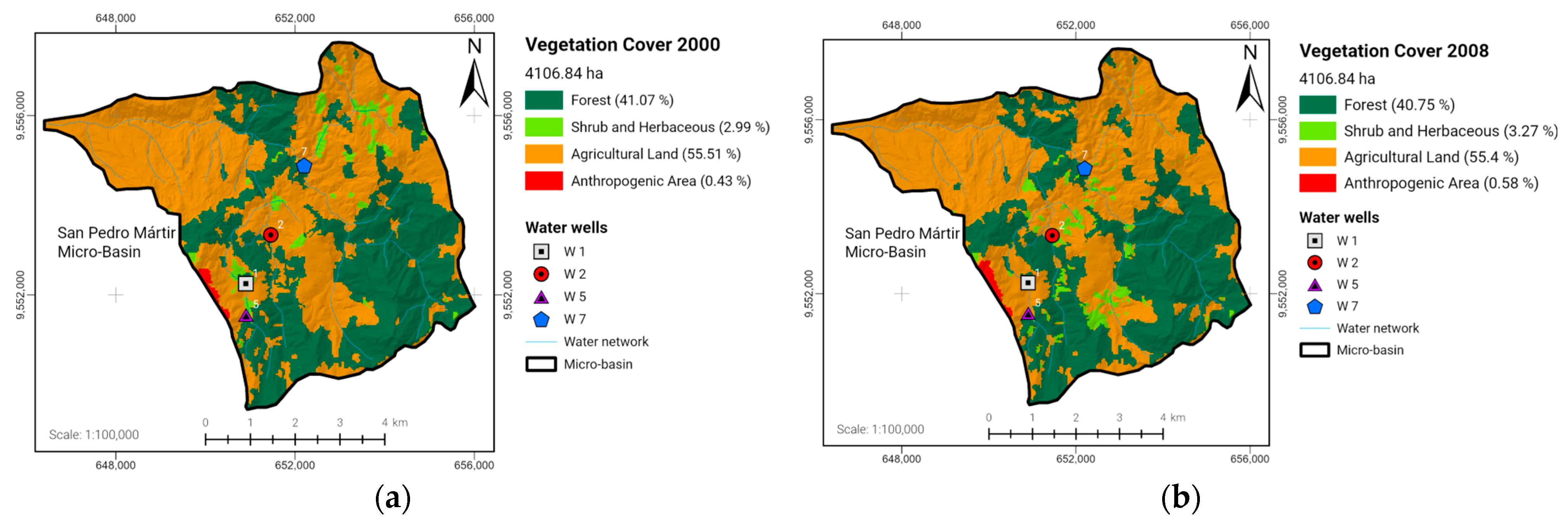
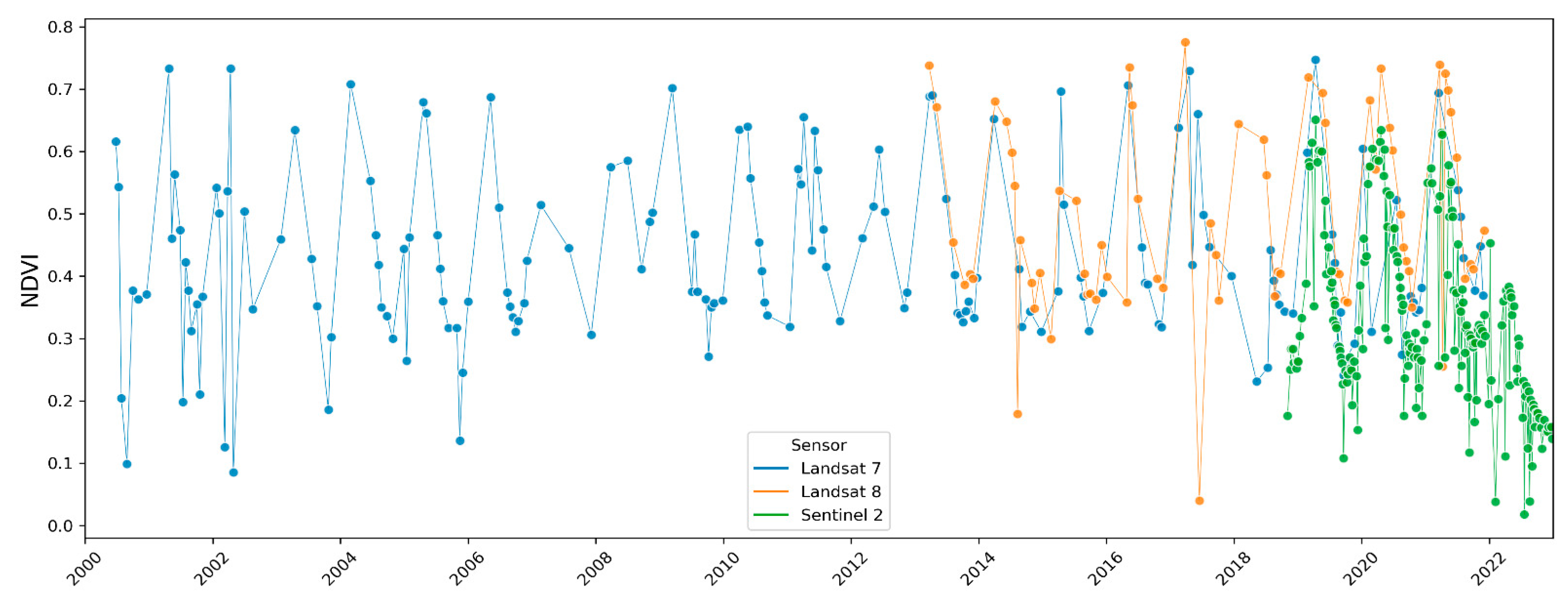
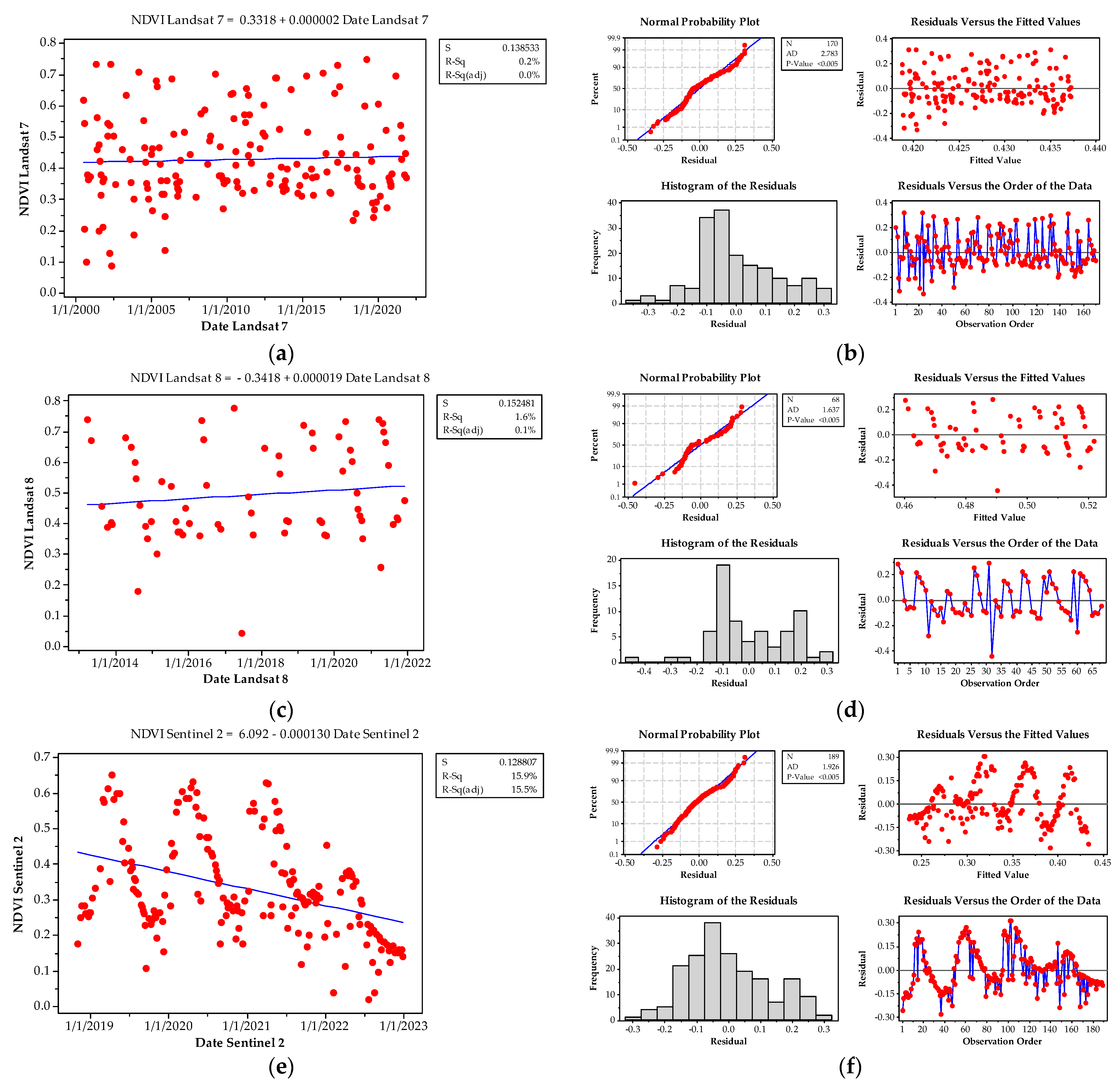
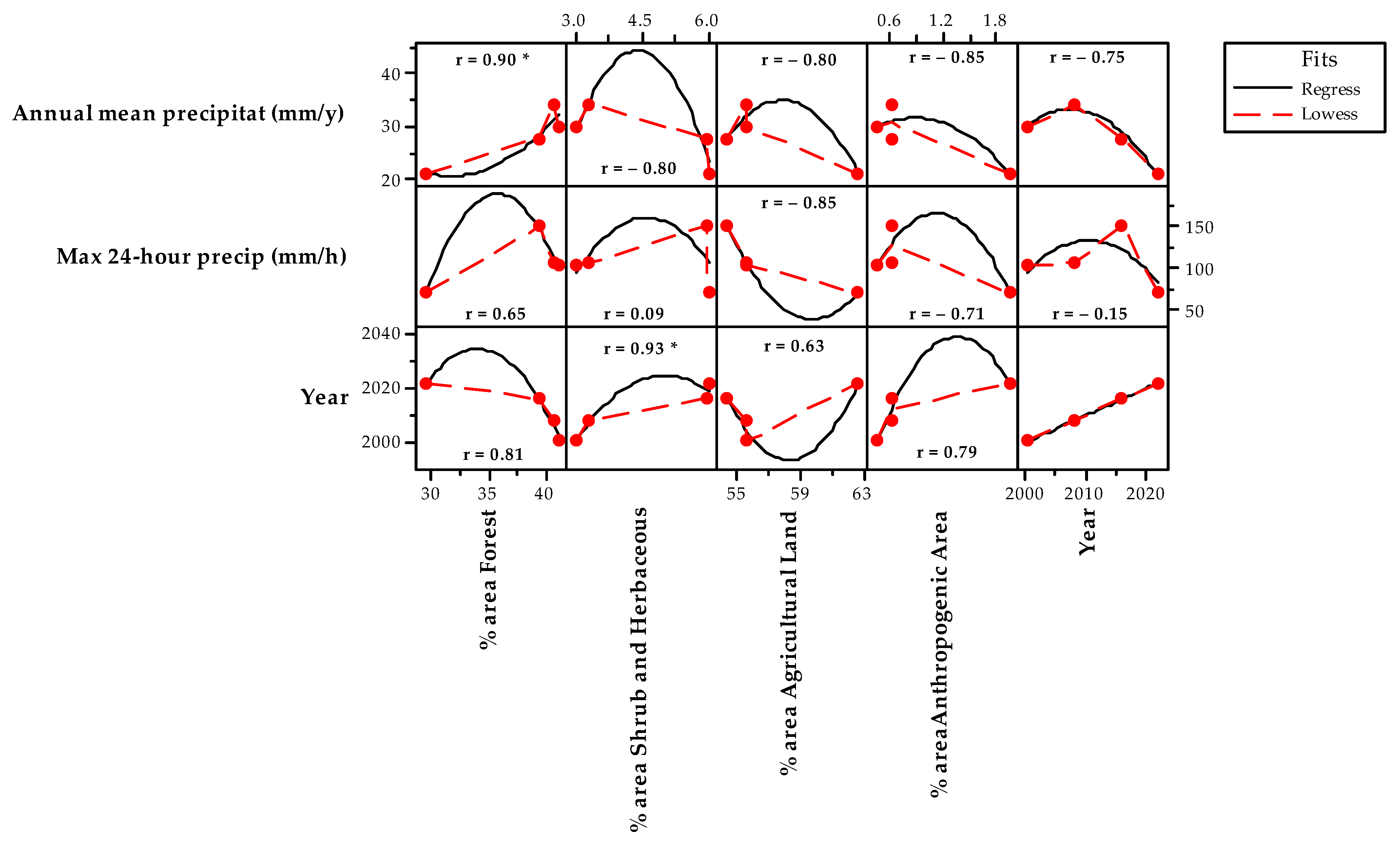
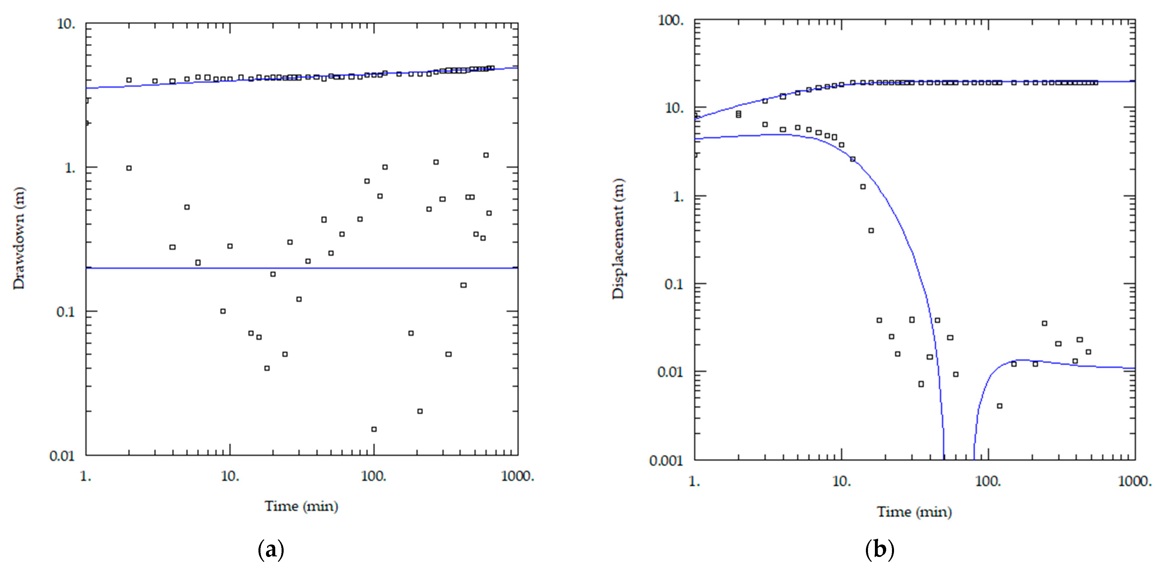
Table 1.
Location of underground wells.
| Well Number | Coordinates | Altitude | Drill Depth | Specific Yield | |
|---|---|---|---|---|---|
| Longitude | Latitude | m a.s.l. | m | (Discharge L/s) % | |
| Well 1 Consacola | −79.64222 | −4.04675 | 1776 | 200 | (2.00 L/s) 32.67% |
| Well 2 Chapango | −79.63567 | −4.03995 | 1691 | 130 | (2.00 L/s) 59.29% |
| Well 5 Santa Marianita | −79.64060 | −4.05577 | 1795 | 170 | (1.08 L/s) 32.67% |
| Well 7 San Pedro Mártir | −79.62659 | −4.01992 | 1640 | 142 | (2.00 L/s) 34.93% |
Table 2.
Aquifer and well performance metrics for the wells in the studio (2004).
| Well | Discharge [L/s] | Aquifer Loss (BQ) [m] | Well Loss (CQ²) [m] | Drawdown (BQ + CQ²) [m] | Specific Yield [%] | Specific Capacity [m³/d/m] |
|---|---|---|---|---|---|---|
| 1 | 0.75 | 5.53 | 4.28 | 9.81 | 56.41 | 6.60 |
| Consacola | 1.00 | 7.38 | 7.60 | 14.98 | 49.25 | 5.77 |
| B = 8.54 × 10⁻² | 1.50 | 11.07 | 17.11 | 28.18 | 39.28 | 4.60 |
| C = 1.02 × 10⁻³ | 2.00 | 14.76 | 30.42 | 45.18 | 32.67 | 3.83 |
| 2 | 1.00 | 3.51 | 1.20 | 4.71 | 74.44 | 18.33 |
| Chapango | 1.50 | 5.26 | 2.71 | 7.97 | 66.01 | 16.25 |
| 2.00 | 7.02 | 4.82 | 11.84 | 59.29 | 14.60 | |
| B = 4.06 × 10⁻² | 2.75 | 9.65 | 9.11 | 18.76 | 51.44 | 12.66 |
| C = 1.61 × 10⁻⁴ | 3.50 | 12.28 | 14.76 | 27.04 | 45.42 | 11.18 |
| 5 | 0.50 | 0.20 | 1.88 | 2.08 | 9.41 | 20.79 |
| Sta. Marianita | 0.67 | 0.26 | 3.38 | 3.64 | 7.20 | 15.89 |
| 0.83 | 0.32 | 5.19 | 5.51 | 5.89 | 13.01 | |
| B = 4.53 × 10⁻³ | 1.08 | 0.42 | 8.78 | 9.21 | 4.59 | 10.14 |
| C = 1.01 × 10⁻³ | 1.33 | 0.52 | 13.32 | 13.84 | 3.76 | 8.30 |
| 7 | 1.00 | 2.90 | 2.71 | 5.61 | 51.78 | 15.40 |
| San Pedro | 1.50 | 4.36 | 6.09 | 10.44 | 41.72 | 12.41 |
| Mártir | 2.00 | 5.81 | 10.82 | 16.63 | 34.93 | 10.39 |
| 2.50 | 7.26 | 16.91 | 24.17 | 30.04 | 8.94 | |
| B = 3.36 × 10⁻² | 3.00 | 8.71 | 24.35 | 33.06 | 26.36 | 7.84 |
| C = 3.62 × 10⁻⁴ | 4.00 | 11.62 | 43.29 | 54.91 | 21.16 | 6.29 |
Note(s): B denotes the circulation loss coefficient within the formation, signifying losses in the aquifer. Its magnitude relies on wellbore diameter, variations in penetration, the presence of heterogeneities, and nearby barriers, primarily. B exhibits variability over the course of pumping. C represents the well loss coefficient, contingent on the type of filter zone, the percentage and arrangement of openings, the extent of aquifer development, and water flow within the wellbore tube until it reaches the pump. C functions as an indicator of the effectiveness of well development [34]. As a guideline for well construction conditions: Values of C ≤ 1.87 × 10⁻³ indicate a well that is well-constructed and developed. Values between 1.87 × 10⁻³ and 3.73 × 10⁻² suggest the onset of encrustations on the well screen. For values ranging from 3.73 × 10⁻² to 1.49 × 10⁻¹, deep well rehabilitation is required due to encrustations or blockage of the well screen. Finally, C values > 1.49 × 10⁻¹ indicate that well rehabilitation is considered very difficult or impossible due to severe encrustations on the well screen.
Table 3.
Classification of vegetation types for the periods 2004 and 2016, according to the reforestation plan [26].
Table 3.
Classification of vegetation types for the periods 2004 and 2016, according to the reforestation plan [26].
| Well | Vegetation Type | 2004 | 2016 | Change over the Period (%) |
|---|---|---|---|---|
| Area (ha) | Area (ha) | |||
| Well 1 | Shrubland | 15.21 | 8.85 | −41.81 |
| Consacola | Urban area and bare soil | 8.23 | 68.40 | 731.11 |
| Cropland | 56.59 | 96.36 | 70.28 | |
| Natural vegetation | 65.00 | 20.72 | −68.12 | |
| Reforestation | 98.43 | 49.13 | −50.09 | |
| Well 2 | Shrubland | 58.27 | 70.12 | 20.34 |
| Chapango | Urban area and bare soil | 9.26 | 121.80 | 1215.33 |
| Cropland | 108.64 | 109.20 | 0.52 | |
| Natural vegetation | 96.91 | 7.90 | −91.85 | |
| Reforestation | 71.90 | 35.96 | −49.99 | |
| Well 5 | Shrubland | 14.85 | 4.15 | −72.05 |
| Santa Marianita | Urban area and bare soil | 6.46 | 54.77 | 747.83 |
| Cropland | 52.35 | 72.21 | 37.94 | |
| Natural vegetation | 46.74 | 20.32 | −56.53 | |
| Reforestation | 61.94 | 30.89 | −50.13 | |
| Well 7 | Shrubland | 398.97 | 558.19 | 39.91 |
| San Pedro Mártir | Urban area and bare soil | 71.05 | 468.80 | 559.82 |
| Cropland | 365.15 | 222.61 | −39.04 | |
| Natural vegetation | 275.24 | 27.61 | −89.97 | |
| Reforestation | 333.65 | 166.85 | −50.00 |
Note(s): Table 3 shows the changes in the extent of different vegetation types in the study area between 2004 and 2016 [26]. According to the data from this reforestation plan report, on average for the study area, shrubland decreased by −10.72%, while urban area and bare soil increased significantly by 650.82%. Cropland rose moderately by 13.94%, and natural vegetation notably declined by −61.29%. In 2016, reforestation and replanting of individuals covered, on average, only 50% of the designated area for this activity, 282.83 ha. These findings suggest that the study area has undergone significant changes in land cover, with a decrease in scrub and cropland and an increase in urban area, bare soil, natural vegetation, and reforestation. Urban development and deforestation are identified as the main drivers of these changes.
Table 4.
Comparison of well flow rates.
| Well | Number | Time (minutes) | Period | Flow (L/s) |
|---|---|---|---|---|
| Consacola | 1 | 16 | 2004 | 4.50 |
| 2016 | 4.57 | |||
| Chapango | 2 | 90 | 2004 | 2.42 |
| 2016 | 2.31 | |||
| Santa Marianita | 5 | 90 | 2004 | 1.50 |
| 2016 | 1.96 | |||
| San Pedro Mártir | 7 | 90 | 2004 | 2.50 |
| 2016 | 2.76 |
Note(s): Table 4 shows the variations in the flow of wells within the designated study area in the years 2004 and 2016. The most remarkable modification observed was the enhancement in the flow rate of the well situated in San Pedro Mártir, which encountered a rise of 12%. In contrast, the well in Chapango experienced a reduction in its flow rate of 4%. Conversely, the flow rates of the wells in Consacola and Santa Marianita exhibited increments of 1.5% and 30%, respectively.
Table 5.
Interpretation of coefficient C in well performance for the years 2004 and 2016.
| Well | Year | Coefficient of Losses in the Well C | Interpretation of Coefficient C |
|---|---|---|---|
| 1 | 2004 | 0.0010 | Well properly constructed and developed |
| Consacola | 2016 | 0.0100 | Initiation of encrustations on wellbore screens |
| 2 | 2004 | 0.0002 | Well properly constructed and developed |
| Chapango | 2016 | 0.0022 | Initiation of encrustations on wellbore screens |
| 5 | 2004 | 0.0010 | Well properly constructed and developed |
| Sta Marianita | 2016 | 0.0052 | Initiation of encrustations on wellbore screens |
| 7 | 2004 | 0.0034 | Initiation of encrustations on wellbore screens |
| San Pedro Mártir | 2016 | 0.0170 | Initiation of encrustations on wellbore screens |
Disclaimer/Publisher’s Note: The statements, opinions and data contained in all publications are solely those of the individual author(s) and contributor(s) and not of MDPI and/or the editor(s). MDPI and/or the editor(s) disclaim responsibility for any injury to people or property resulting from any ideas, methods, instructions or products referred to in the content. |
© 2024 by the authors. Licensee MDPI, Basel, Switzerland. This article is an open access article distributed under the terms and conditions of the Creative Commons Attribution (CC BY) license (https://creativecommons.org/licenses/by/4.0/).
Share and Cite
MDPI and ACS Style
Benavides-Muñoz, H.M.; Correa-Escudero, V.; Pucha-Cofrep, D.; Pucha-Cofrep, F. Analysis of Land Use Change and Hydrogeological Parameters in the Andean Semiarid Region of Ecuador. Water 2024, 16, 892. https://doi.org/10.3390/w16060892
AMA Style
Benavides-Muñoz HM, Correa-Escudero V, Pucha-Cofrep D, Pucha-Cofrep F. Analysis of Land Use Change and Hydrogeological Parameters in the Andean Semiarid Region of Ecuador. Water. 2024; 16(6):892. https://doi.org/10.3390/w16060892
Chicago/Turabian StyleBenavides-Muñoz, Holger Manuel, Verónica Correa-Escudero, Darwin Pucha-Cofrep, and Franz Pucha-Cofrep. 2024. "Analysis of Land Use Change and Hydrogeological Parameters in the Andean Semiarid Region of Ecuador" Water 16, no. 6: 892. https://doi.org/10.3390/w16060892
Note that from the first issue of 2016, this journal uses article numbers instead of page numbers. See further details here.