Monitoring and Early Warning Method of Debris Flow Expansion Behavior Based on Improved Genetic Algorithm and Bayesian Network

Abstract

Based on an improved genetic algorithm and debris flow disaster monitoring network, this study examines the monitoring and early warning method of debris flow expansion behavior, divides the risk of debris flow disaster, and provides a scientific basis for emergency rescue and post-disaster recovery. The function of the debris flow disaster monitoring network of the spreading behavior disaster chain is constructed. According to the causal reasoning of debris flow disaster monitoring information, the influence factors of debris flow, such as rainfall intensity and duration, are selected as the inputs of the Bayesian network, and the probability of a debris flow disaster is obtained. The probability is compared with the historical data threshold to complete the monitoring and early warning of debris flow spreading behavior. Innovatively, by introducing niche technology to improve traditional genetic algorithms by learning Bayesian networks, the optimization efficiency and convergence speed of genetic algorithms are improved, and the robustness of debris flow monitoring and warning is enhanced. The experimental results show that this method divides debris flow disasters into the following five categories based on their danger: low-risk area, medium-risk area, high-risk area, higher-risk area, and Very high-risk area. It accurately monitors the expansion of debris flows and completes early warning. The disaster management department can develop emergency rescue and post-disaster recovery strategies based on early warning results, thus providing a scientific basis for debris flow disasters. The improved genetic algorithm has a higher learning efficiency, a higher accuracy, a faster convergence speed, and higher advantages in learning time and accuracy of the Bayesian network structure.

1. Introduction

A debris flow disaster is destructive and sudden and can seriously damage property, facilities, and the natural environment in flowing areas [1], pose a significant threat to the life and safety of residents, and cause a lot of economic losses [2]. Therefore, it is urgent to study the risk of debris flow disasters in depth and reduce the disaster risk [3]. Bernard M. et al. [4] predicted an occurrence of debris flows through rain gauge measurement and radar data, normalized the collected rainfall data, input it into the established debris flow early warning function, and generated early warning information according to the prediction result of the function. However, this method does not comprehensively collect data on debris flows, which leads to low prediction accuracy. Savi M. et al. [5] used the delayed acceptance algorithm to predict the debris flow based on historical data and statistical functions to predict the occurrence probability and influence the range of debris flow expansion behavior. However, this method is not effective in learning the structure of debris flow disaster monitoring networks, and it is prone to the phenomenon of edge loss and multilateralism, resulting in inaccurate prediction results. Nagl et al. [6] monitored the protection structure of debris flow, determined the objective function of prediction, and then used a hill climbing algorithm to complete the monitoring of debris flow expansion behavior. However, the global search ability of this method is poor, and the iteration speed is slow; thus, the solution effect of the complex problem of debris flow expansion behavior is not ideal. Coviello V. et al. [7] monitored the spreading behavior of debris flow through the combination of the Gale–Shapley algorithm and the debris flow disaster monitoring network, combined with high-resolution terrain and instruments. Although this method is simple and easy to operate, the number of wrong edges in the structure of the debris flow disaster monitoring network is large, and the learning effect is not decent. Rui et al. [8] used the minimum spanning tree method to calculate the weight of debris flow occurrence time and rainfall change to complete the prediction. However, this method takes a long time to calculate, and the learning effect of the debris flow disaster monitoring network structure is poor. Ya-Q J [9] used high-frequency pulse radar as a monitoring tool to detect layered land media, extracting important stimuli for debris flows and landslides. A layered land medium model with random scattering bodies embedded with random rough interfaces was constructed, and numerical simulations were conducted on the polarization radar distance profiles of underground structures under different conditions to early monitor and warn of debris flow disasters. Wang X [10] proposed a debris flow warning method based on the infinite independence method and self-organizing feature mapping and applied it to Liaoning Province. The proposed model consists of three stages. Firstly, by analyzing the factors that affect the development of debris flows in the study area, eight geological environmental conditions and two rainfall-induced conditions were selected. The rainfall threshold for debris flow outbreaks was 150 mm, avoiding the blindness of parameter selection and conducting monitoring and early warning.

Because the network function of debris flow disaster monitoring has a strong ability to analyze uncertain problems, it can not only synthesize various factors to complete the assessment but can also visually show the logical relationship between factors in a graphic way, which has been widely used in disaster risk management. Therefore, this paper proposes a monitoring and early warning method for debris flow expansion behavior based on the improved genetic algorithm and debris flow disaster monitoring network.

2. Debris Flow Expansion Behavior Monitoring and Early Warning

2.1. Debris Flow Disaster Monitoring Network Node Variable Analysis

To construct the monitoring network function of the debris flow extended behavior disaster chain, first, it is necessary to establish the monitoring network diagram of the debris flow disaster and then realize the probability prediction of the debris flow disaster by causal reasoning.

Appropriate factors affecting debris flow spreading behavior were selected as parameters to optimize the performance of the function. According to the data reported by the national disaster reduction network, local government websites, Baidu Encyclopedia, and other authoritative websites, and combined with expert opinions, the node variables of common influencing factors of debris flow expansion behavior were selected, as shown in

Table 1. Variables of the debris flow disaster chain.

Variable Type	Variable
Input variables	Rainfall intensity
	Rainfall duration
State variable	Lithological structure
	Geological structure
	Loose soil
	Topographic features
	Original water system
Output variables	Debris flow

.

We searched the keywords of debris flow disaster nodes, obtained the relevant disaster literature, and obtained the influencing factors of debris flow disaster nodes.

2.2. Improved Early Warning Method of Genetic Algorithm Based on Niche Technology

2.2.1. Optimization of Variable Factors of Debris Flow Expansion Behavior

The relationship between factors influencing mudslide dispersal behavior and the choice of conditional probability distribution can easily influence monitoring networks. Therefore, it is necessary to find the best parameter set (variable factors of debris flow expansion behavior) to make the early warning function have the best performance.

For given monitoring information, let the objective function be [11,12]:

$$F=f(x,y,z),\hspace{1em}(x,y,z)\in \Omega ,\hspace{0.17em}F\in R$$

(1)

In order to make the objective function of formula (1) not lose generality, it can be assumed that the minimum value is sought; that is:

$$F^{\prime }=\underset{(x,y,z)\in \Omega }{\min }f(x,y,z)$$

(2)

In the formula, $x,y,z$ are independent variables, which can be quantities or symbols; Ω is the domain of $x,y,z$, which can also be regarded as the solution space composed of all possible solutions of the problem, which is a measure of the quality or fitness of the solution; $F^{\prime }$ is a real number; $f$ is a mapping from solution space $(x,y,z)\in \Omega$ to real number field $F\in R$.

Genetic algorithms can perform a parallel search by simultaneously processing multiple candidate solutions, thereby accelerating the search speed. With the help of parallel search, genetic algorithms can search for globally optimal or near optimal solutions in a relatively short amount of time. Genetic algorithms have a strong global search ability and can find the global optimal solution in complex, multi-modal, and nonlinear problems. Through continuous evolution and crossover operations, genetic algorithms can traverse the search space and gradually tend towards better solutions. In summary, using genetic algorithms to search for the optimal parameters can effectively find the complex optimization problem of the prior probability of the optimal parameter set for debris flow expansion behavior through parallel and global search capabilities. Therefore, using genetic algorithms to search for prior probabilities in the debris flow disaster monitoring network plays an important role in monitoring the debris flow expansion behavior of the debris flow disaster monitoring network, and it can adjust the parameters of the debris flow disaster monitoring network. However, it is prone to local optimization and unable to utilize feedback from debris flow monitoring networks in a timely manner. Based on this, niche technology was introduced to improve the traditional genetic algorithm and its optimization efficiency and convergence speed.

The steps of improving the genetic algorithm by combining dynamic niche sharing algorithm are as follows:

Step 1: Process the data of the training debris flow disaster nodes and construct the residual according to the constructed simulation equation format.

Step 2: Calculate the fitness values and arrange them in descending order.

Step 3: Niche selection: Take the first individual in descending order as the first niche center, respectively calculate the Euclidean distances between other individuals and the niche center, and if the distance is greater than a given value L and the existing niche center is less than a given value $K$, then the individual becomes a new niche center. If the distance between the individual and the niche center is less than the fixed value L, then the individual is regarded as the niche individual. If the distance between an individual and a niche is greater than L and the number of niche centers is greater than or equal to K, the individual becomes an independent individual.

Step 4: Niche mirror processing: If an individual is in a niche mirror, then its niche number is the number of individuals in its niche, and the niche center and the niche number of individuals are specified as 1.

Step 5: Calculate the fitness value after sharing.

Step 6: Carry out a population adaptive crossover operation.

Step 7: Perform a population adaptive mutation operation.

Step 8: If the termination judgment condition is met, output; if the termination condition is not met, skip to step 2 and perform loop operations until the algorithm is terminated.

Where the construction difference in step 1 is a defined polynomial after the random number $x,y$ of the simulation [13,14]:

$$y_i=a{x}^3+b{x}^2+cx+d$$

(3)

The simulated good random number $x$ is replaced into the $y$ of the simulation.

The structural difference is:

$$\min g\left(a,b,\dots \right)={\displaystyle \sum }_{i=0}^n{(f\left(x_i;a,b,\dots \right)-y_i)}^2$$

(4)

Among $g$ is the simulated function $f$, is the template of the simulation function, $a,b,\dots$ They are the coefficients of the simulation function, in which the Euclidean distance in step 3 is calculated as follows:

$$\Omega =\sqrt{{\displaystyle \sum }_{i=1}^n\min g\left(a,b,\dots \right){(x_i-y_i)}^2}$$

(5)

The formula for recalculating the fitness value in step 5 is as follows:

$$f(x)=\{\begin{array}{l}F(x)/S(x),\hspace{0.17em}\hspace{0.17em}\Omega (x_i)<L\\ F(x),\hspace{0.17em}\hspace{0.17em}\Omega (x_i)\ge L\end{array}$$

(6)

Among $F\left(x\right)$ is a function that describes the level of individual fitness. $S\left(x\right)$ is shared functions, and $\Omega \left(x_i\right)$ is the Euclidean distance between data, which is the niche number in this algorithm. Because many similar data affect the influencing factors of debris flow expansion behavior in the experiment, we can find similar data by calculating the Euclidean distance between the data. After recalculating the fitness value of the data, we can narrow the fitness value of similar data, which can reduce the similar data in the influencing factors of debris flow expansion behavior, thus increasing the diversity of data and avoiding it.

In step 6 and step 7, the traditional genetic algorithm is a fixed value, and the probability of crossover and mutation after the introduction of niche technology to improve the genetic algorithm in an innovative way is as follows [15]:

$$pc=\left\{\begin{array}{l}{k}_i\frac{f\max -f}{f\max -favg},\hspace{0.17em}f\ge favg\\ k_3,\hspace{0.17em}f<favg\end{array}\right\},\hspace{1em}pm=\left\{\begin{array}{l}{k}_2\frac{f\max -f^{\prime }}{f\max -favg},\hspace{0.17em}{f}^{\prime }\ge favg\\ k_4,\hspace{0.17em}{f}^{\prime }<favg\end{array}\right\}$$

(7)

Among $pc$, $pm$ are the probabilities of crossover and mutation operations; f_max is the largest fitness value in the population; $f$ is the fitness value of the individual to be crossover operated; $f\mathrm{avg}$ is the average fitness value of the population; $f^{\prime }$ is the fitness value for the mutation operation; $k_1,\hspace{0.17em}{k}_2,\hspace{0.17em}{k}_3,\hspace{0.17em}{k}_4$ are constants; in combination with $\mathrm{si}gmoid$, the probability of the crossover and mutation of the improved function is as follows:

$$\mathrm{pc}=k_1\frac{1}{1+e^{-\left(favg-f\right)}},\mathrm{pm}=k_2\frac{1}{1+e^{-\left(favg-f^{\prime }\right)}}$$

(8)

As an example, the crossover probability of the adaptive genetic algorithm is unchanged when the fitness value of the individual is smaller than the average fitness value of the population. In the improved adaptive genetic algorithm, the crossover probability of individual populations will vary with the fitness value of individual populations, and the smaller the fitness value of individual populations, the greater the crossover probability.

When the fitness value of individual populations is greater than the average fitness value:

$$\mathrm{pc}\left(AGA\right)=K\frac{f\max -f}{f\max -fa\nu g}=k\left(1+\frac{fa\nu g-f}{f\max -fa\nu g}\right)$$

(9)

$Suppose x=fa\nu g-f, u=f\max -fa\nu g\left(u\ge 0,x\le 0,u\ge -x\right)$, and:

$$pc\left(AGA\right)=K\left(1+\frac{x}{u}\right)$$

(10)

The probability of crossover of the improved algorithm is:

$${\mathrm{p}\mathrm{c}}^{\prime }=\frac{1}{1+e^{-\left(favg-f\right)}}$$

(11)

Make $x=fa\nu g-f\left(x\le 0\right)$; then $pc=k\frac{1}{1+e^{-x}}$, and there are:

$$F\left(x\right)=pc-pc\left(AGA\right)=k\left(\frac{1}{1+e^{-X}}-1-\frac{x}{u}\right)$$

(12)

In the improved genetic algorithm, when the fitness value of individuals is greater than the average fitness value, compared to the traditional genetic algorithm, the improved genetic algorithm can reduce the probability of cross mutation, thus preserving the integrity of individuals and making the fitness value of individuals more significant than the average fitness value, changing the mutation probability according to the fitness value changes and increasing the population convergence speed.

The traditional genetic algorithm has the characteristic of weak search ability, and it easily falls into local optimal solution; thus, innovation is achieved by using the $sigmoid$ function in the improved genetic algorithm, and the probability of crossover and mutation is calculated according to the fitness value of individuals, so that the probability of crossover and mutation has a high convergence speed, thus accelerating the ability of the global optimization of the algorithm.

2.2.2. Bayesian Network Learning under Global Optimization

In order to ensure the effectiveness and diversity of the initial population (Bayesian network structure) of the improved genetic algorithm when learning the Bayesian network, the initial population is divided into two parts according to the Bayesian network structure. In part, the maximum weight tree of the Bayesian network structure is obtained by mutual information calculation. The direction of the edges in the maximum weight tree is determined by the scoring function. The individuals in the neighborhood are generated by adding, deleting, and reversing edges to the maximum weight tree. At the same time, to ensure the diversity of the initial population and prevent it from falling into local optimum prematurely in the process of population search, the other part ensures the diversity of the population by randomly generating some individuals.

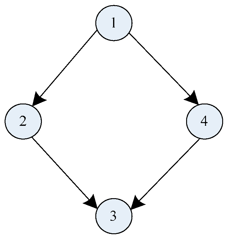
A Bayesian network is matrix coded by introducing Bayesian, and the form of the adjacency matrix is adopted [16]:

$$\begin{gathered} \mathrm{A}=\left[\begin{array}{cc}\begin{array}{cc}0& 1\\ 0& 0\end{array}& \begin{array}{cc}1& 0\\ 0& 1\end{array}\\ \begin{array}{cc}0& 0\\ 0& 0\end{array}& \begin{array}{cc}0& 1\\ 0& 0\end{array}\end{array}\right] \\ a\left(i,j\right)=\{\begin{array}{ll}1\hfill & i\mathrm{is}\mathrm{the}\mathrm{parent}\mathrm{node}\mathrm{of}\mathrm{j}\hfill \\ 0\hfill & \mathrm{Others}\hfill \end{array} \end{gathered}$$

(13)

The mutual information of the random variables $X$ and $Y$ in each node in the debris flow disaster monitoring network is defined as follows:

$$I\left(X;Y\right)=H\left(X\right)-H\left(X|Y\right)$$

(14)

In the formula, $H\left(X\right)$ and $H\left(Y\right)$, respectively, are the information entropy of $X$ and $Y$; $H\left(X|Y\right)$ is the conditional information entropy in a given $Y$ under $X$; and $H\left(X\right)$, $H\left(X|Y\right)$ are defined as follows:

$$H\left(X\right)=-{\displaystyle \sum }_{i=1}^n\mathrm{P}\left(F{\left(x\right)}_i\right)\log \left(P\left(X_i\right)\right)$$

(15)

$$H\left(X|Y\right)=-{\displaystyle \sum }_{i=1}^n{\displaystyle \sum }_{j=1}^{m}P\left(X=x_i,Y=y_i\right)\cdot \log (P(X=x_i|Y=y_i))$$

(16)

Formula $P\left(X_i\right)$ represents a probability function.

Because the mutual information value has the nature of commutative law (that is $I\left(X;Y\right)=I\left(Y;X\right)$, so it has $n$ structure of debris flow and the disaster monitoring network of nodes needs to be calculated $C_n^2$ times), the greater the mutual information value, the stronger the correlation between the two nodes, the stronger the correlation between the influencing factors of debris flow expansion behavior input in the nodes, and the greater the possibility that there is an edge between the nodes. However, the direction of the edge cannot be determined, and it is an undirected graph.

Randomly determining the direction of the edge is not conducive to the search efficiency of the algorithm. In order to determine the direction of the edge, the connected nodes in the maximum weight tree are used as parent nodes and child nodes once, respectively, through the scoring function $BIC$ to calculate the function values in turn, and they select the maximum value as the edge direction.

The scoring function $BIC$ is to comprehensively consider the complexity and matching degree of the Bayesian network, so that it can obtain more accurate early warning results of debris flow expansion behavior [17,18].

$$Q_{BIC}={\displaystyle \sum _{i=1}^n\log P(}B|D)I(X;Y)-1/2\mathrm{l}ogN\cdot Dim(B)$$

(17)

Formula $B$ represents the learned Bayesian network structure, and $D$ is the collected data set of debris flow expansion behavior. In order to homogenize, the node pairs are selected by chaotic mapping to add, delete, and reverse edges, resulting in the initial population.

Because chaotic thought has the characteristic of traversing all regions, compared with $Logistic$ mapping and $Tent$ mapping, the $Kent$ chaotic map has a more uniform distribution over the (0, 1.0) interval, and it will not fall into the periodic point. Therefore, this paper adopted the $Kent$ chaos mapping, which is used to select the nodes of the debris flow disaster monitoring network. The chaotic mapping formula of $Kent$ is as follows:

$$x\left(n+1\right)=\{\begin{array}{ll}\frac{Q_{BIC}x\left(n\right)}{\beta }\hfill & 0<x\left(n\right)\le \beta \hfill \\ \frac{\left(1.0-Q_{BIC}x\left(n\right)\right)}{\left(1.0-\beta \right)}\hfill & \beta <x\left(n\right)\le 1.0\hfill \end{array}$$

(18)

In the formula, $x$ is a chaotic sequence; $\beta$ is set a parameter. When $\beta =0.4$, then the index $Lyapunov$ is about 0.696, and the probability density function is uniformly distributed in interval (0,1.0), as shown in Figure 1.

The monitoring network of debris flow disaster has $n$ nodes, $Kent$ mapping generates random numbers ${\gamma }_{\mathrm{i}}\in (0,1)$, and the following formula is used to select nodes and add, delete, and reverse edges.

$$x_i(0)=ceil(r\ast n)x(n+1)\hspace{1em}i=1,2,\dots n$$

(19)

The additive operation in the $B$ of the encoding matrix of the Bayesian network is expressed as $B\left(i,j\right)=1$. The deleted edge is represented by $B\left(i,j\right)=0$; the reverse edge is represented by $B\left(i,j\right)=0$ and makes $B\left(j,i\right)=1$.

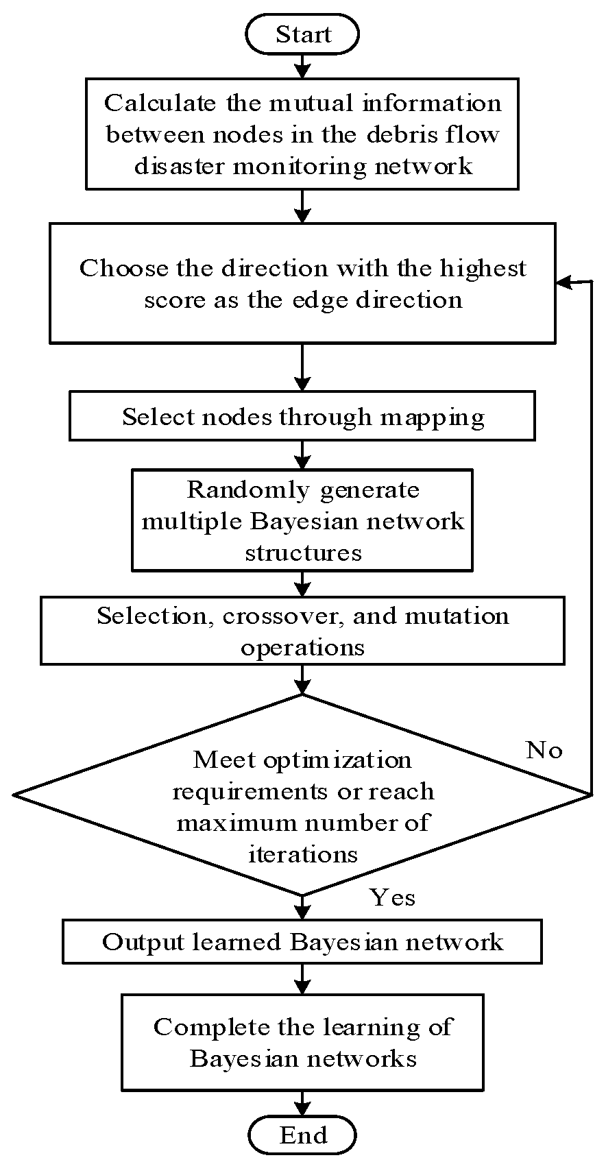
For the debris disaster monitoring network structure of $n$ nodes, the specific steps of learning the Bayesian network are as shown in Figure 2.

(1) By calculating the mutual information between the nodes of the debris flow disaster monitoring network [19], select the maximum (n − 1) side of the mutual information.

(2) Through the BIC scoring function, which takes two nodes of each edge as parent nodes and child nodes, respectively, for scoring calculation, select the direction with the largest score as the direction of the edge.

(3) Through the Kent chaotic mapping, select nodes i and j, such as B(i,j) = 1 ∪ B(j,i) = 1, reverse edges, and trim edges, such as B(i,j) = 0, and then add edges.

(4) Randomly generate a plurality of Bayesian network structures to join the initial population to form the latest population.

(5) Selection, crossover, and mutation operations: Select better individuals, select column vectors of the adjacency matrix by the Kent mapping, perform crossover operations, select individuals according to probability for mutation operations, increase population diversity, and correct illegal graphs generated by population individuals in the process of crossover and mutation to ensure the legalization of topological structure. When the population does not produce a new optimal solution for many times, the mutation intensity is increased to make it jump out of the local optimum.

(6) Repeat step (5) until the termination conditions are met (optimization requirements are met or the maximum number of iterations is reached).

(7) Output the learned Bayesian network and use the Bayesian network with optimal parameters and reasoning ability [20].

2.2.3. Hierarchical Early Warning Method Based on Bayesian Network Learning Results

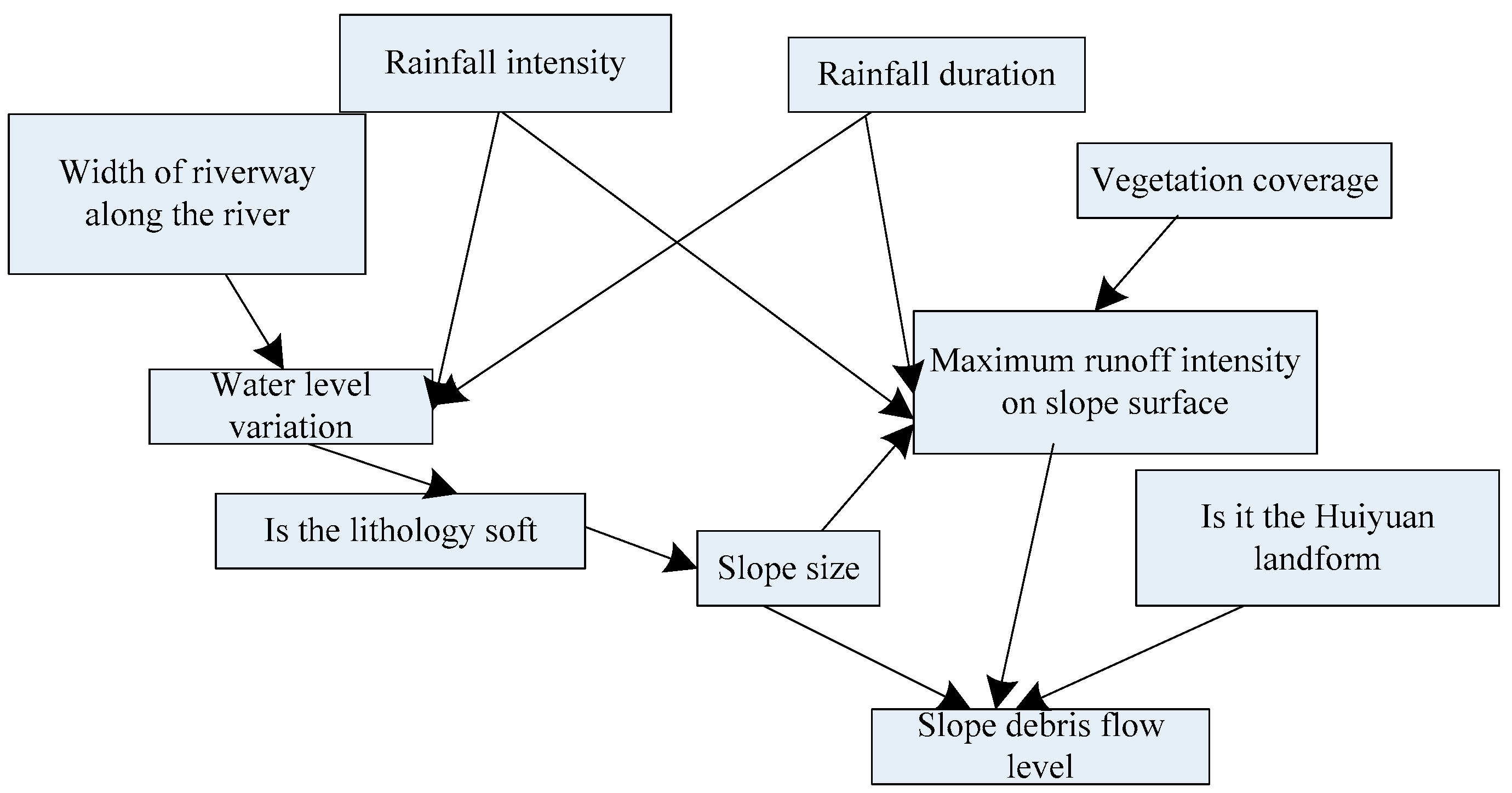
Based on this, the causal relationship of each node in the debris flow disaster monitoring network structure is constructed, and the Bayesian network topology structure of the debris flow disaster chain is obtained, as shown in Figure 3.

Causal reasoning of the monitoring and early warning of debris flow expansion behavior uses the forward causal reasoning technology of the Bayesian network to calculate the conditional probability of the occurrence of child nodes (debris flow disaster) when the state of the parent node (influencing factors of debris flow expansion behavior) is known, that is, to predict. Based on the constructed Bayesian network diagram, the conditional probability of child nodes of debris flow secondary disaster in different states is calculated when the parent node of the debris flow primary disaster is known, and the final risk level of debris flow expansion behavior is obtained. For example, in the process of the debris flow disaster chain reaction, the set of all the parent nodes S_i affecting the occurrence of the disaster node is the influencing factor S_a. In this case, the probability of the secondary disaster child node S_b being in the state₂ state is P(S_b = state₂|Sa), which is calculated as shown in Equation (1).

$$\begin{array}{l}P(S_b={\mathit{state}}_2|S_a)=F^{\prime }{x}_i\left(0\right)P(S_b=stat{e}_1,\dots S_1=stat{e}_1)=\\ \frac{F^{\prime }xi\left(0\right)P\left(S_b=stat{e}_2, S_1=stat{e}_1,\dots S_n=stat{e}_1\right)}{P(S_1=stat{e}_1,\dots ,S_n=stat{e}_1)}\\ S_i\in S_n, stat{e}_i \left(i\in \left[0–4\right]\right)\end{array}$$

(20)

In Formula (1), n is the number of debris flow expansion behavior disaster nodes; each debris flow disaster node has i states; P(S_b = state₂, S₁ = state₁, …, S_n = state₁) represents the probability of the simultaneous occurrence of all debris flow disasters’ parent state state₁ and secondary sub-nodes S_b state state₂; P(S₁ = state₁, …, S_n = state₁) represents the joint probability that the event has occurred and that all the parent node states are state₁.

By analyzing the state of debris flow disaster nodes, parent nodes, and child nodes, the joint probability is calculated by the Bayesian network constructed in this paper, and the possibility of debris flow expansion behavior is converted into specific values. Finally, it is compared with the threshold set by historical data to complete the monitoring and analysis of debris flow expansion behavior. Comparing the calculated joint probability value with the threshold set by historical data, the higher the joint probability, the greater the possibility of debris flow expansion. When the joint probability value is 80–100%, then the risk level is very high, and the Bayesian network function issues an alarm-level warning. When the joint probability value is 60–80%, then the risk level is higher, and an alarm-level warning is issued. When the joint probability value is 40–60%, then risk level is high, and a warning-level warning is issued. When the joint probability value is 20–40%, then the risk level is medium, and a warning-level warning is issued. When the joint probability value is 0–20%, then the risk level is low, and an attention-level warning is issued.

3. Experiment and Analysis

The debris flow disaster caused damage to houses, farmland, river banks, electricity, communications, and other facilities to varying degrees, and traffic, communications, and electricity were interrupted. The landforms in the L area are characterized by the easy occurrence of disasters such as soil erosion, desertification, rocky desertification, and debris flow [21,22,23]. In order to verify the effect of this method on the monitoring and early warning of debris flow spreading behavior, real debris flow samples in this area were collected, and the characteristics of each sample, such as rainfall, rainfall duration, material composition, occurrence time, and place, were recorded in detail. The monitoring and early warning results of this method were compared with the real debris flow in this area. The specific situations of debris flow disasters in this area in 2023 are as follows: (1) Low-risk areas: Three areas in this area are classified as low-risk areas. In these areas, there are few risks and safety problems, and daily life and activities can be basically guaranteed to be normal. (2) Medium-risk areas: Two areas in this area are classified as medium-risk areas. In these areas, there are certain risks and safety problems, but these problems have not seriously affected daily life and activities. (3) High-risk and higher-risk areas: each area in this area is divided into high-risk and higher-risk areas. In these areas, there are relatively many risks and safety problems, which may have a certain impact on daily life and activities. (4) Very high-risk areas: There are two areas in this area that are classified as very high-risk areas. In these areas, the risk and safety problems are extremely serious and may seriously affect normal daily life and activities.

In order to verify the validity of the monitoring and early warning function of debris flow expansion behavior in this paper, the relevant data on debris flow disasters in this area in 2021, such as time and place, were collected through field investigation and equipment. The related factors, such as rainfall and topography, were recorded.

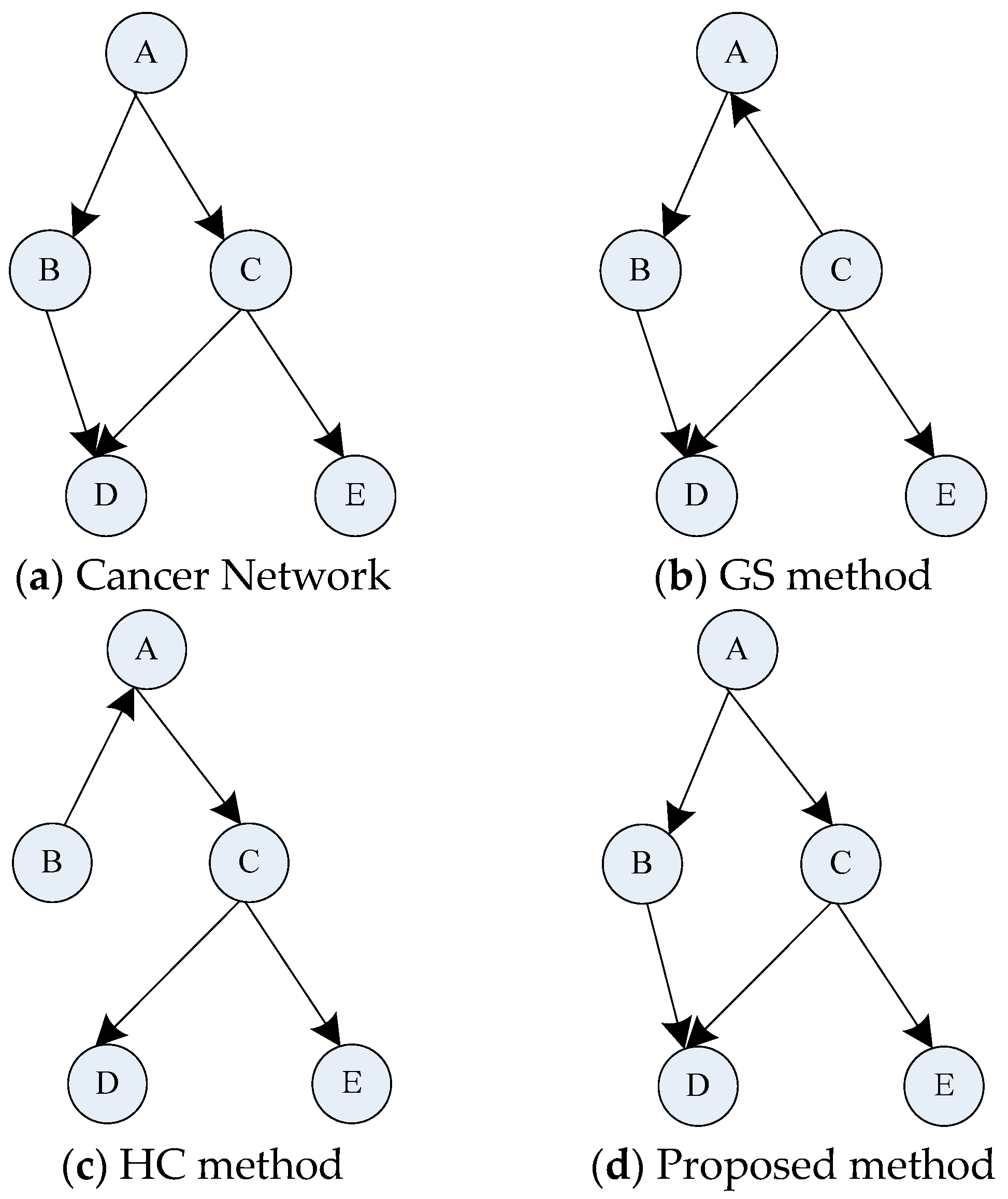
In order to verify the learning effect of the improved genetic algorithm on the Bayesian network structure, taking the Cancer Bayesian network as an example, the number of lost edges, reverse edges, and added edges in the Bayesian network after learning was used as the evaluation index of the Bayesian network structure learning effect. Because of the randomness of the genetic algorithm, this paper adopted 20 experimental results and obtained the average value. Let the population number of the improved genetic algorithms in this study be 50 and the maximum number of iterations be 100. The method in this study was compared with the delayed acceptance method (GS) and hill climbing method (HC). In order to ensure comparability, the experimental results under the same conditions are shown in Figure 4 and

Table 2. Cancer network testing.

Number of Data Groups		GS Method	HC Method	Proposed Method
500	Network Structure Rating	−919.325	−916.537	−912.716
	Missing Edges	0.2	0	0
	Redundant Edge	0	0.1	0
	Reverse Edge	1.6	1.1	0.7
1000	Network Structure Rating	−187.254	−187.254	−187.254
	Missing Edges	0	1	0
	Redundant Edge	0	0	0
	Reverse Edge	0.9	1.1	0.4

.

As can be seen from Figure 4, compared to the standard diagram of the Cancer Bayesian network, the final result of the GS method had a reverse edge, and the final learning result of the HC method had a lost edge and a reverse edge. However, the Bayesian network, after learning that this method does not have the phenomenon of lost edge, multilateral edge, or reverse edge, which shows that the improved genetic algorithm in this method has a good learning effect on the Bayesian network structure.

As seen from

Table 3. Comparison of genetic algorithms.

Index	Network Structure Rating	Average Number of Iterations
Improved Genetic Algorithm	−4966.1	30
Standard Genetic Algorithm	−4988.7	81

, the Bayesian network structure obtained from this method was the least in the cases of the missing edge, multilateral edge, and reverse edge, and the score of the Bayesian network structure was also the highest among the three methods. Moreover, under the same scoring function value, this method had the highest probability of finding the best Bayesian network structure.

In order to verify the effectiveness of the improved genetic algorithm, the improved genetic algorithm and the standard genetic algorithm learned the Bayesian network structure. The initial population size was 50, and the iteration was 100 times. Under the same conditions, 20 experiments were carried out. The score and average iteration times are shown in Table 3, and the iteration curve is shown in Figure 5.

In Table 3, it can be seen that the score of the Bayesian network structure and the average number of iterations were better than the standard genetic algorithm after using the improved genetic algorithm. As seen from the iteration curve comparison diagram in Figure 4, the improved genetic algorithm obtained the optimal result in about 26 iterations, and the standard genetic algorithm needed about 57 iterations to obtain the optimal result. Therefore, the Bayesian network learning method based on the improved genetic algorithm in this paper has the advantages of fewer iterations and faster convergence speed, and the Bayesian network optimized by the improved genetic algorithm was more efficient in the monitoring and early warning of debris flow expansion behavior.

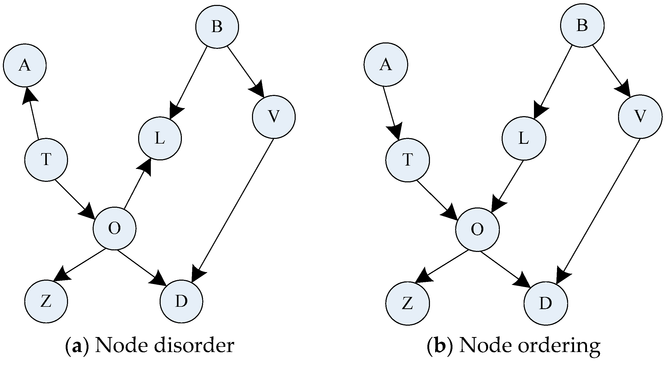
In order to verify the performance of the improved genetic algorithm, this study compared the time performance, accuracy, and the final score of the Bayesian network structure with various algorithms under the same sample conditions. Figure 6 shows the structure obtained by learning the Bayesian network structure with the improved genetic algorithm under the conditions of disorder and order.

The learning results of the improved genetic algorithm are compared with those of the Gale–Shapley algorithm (GA) and Minimum Spanning Tree algorithm (MWST) under the condition of disordered and ordered nodes. The experimental results are shown in

Table 4. Comparison of the learning results of multiple methods.

Learning Method	Learning Time	Wrong Number of Edges	Network Structure Scoring
The method proposed in this paper when nodes are out of order	0.66 s	2	−44,816
The method proposed in this paper when nodes are ordered	0.41 s	0	−44,816
GA method	107.28 s	7	−44,842
MWST method	0.94 s	4	−45,879

.

From Figure 4, it can be seen that the improved genetic algorithm in this paper had the highest Bayesian network structure score and the least number of wrong edges in both cases of ordered and disordered nodes. Regarding learning time, the improved genetic algorithm was better than GA and MWST. Therefore, this method was superior in terms of learning time and accuracy of the Bayesian network structure. The accuracy and efficiency of monitoring and the early warning of debris flow expansion behavior using this method have obvious advantages.

We input the collected data into this method, and the early warning result is shown in Figure 7.

As seen in Figure 7, there are three low-risk areas, two medium-risk areas, one high-risk area, and two very high-risk areas. Compared to the actual on-site data of the debris flow occurrence area in 2021, the monitoring and early warning results of the debris flow disaster in this research method were completely consistent with the debris flow occurrence area in 2021. The experiment verified the effectiveness of this method in the monitoring and early warning of debris flow expansion behavior.

The joint probability value and risk grade of debris flow disasters in counties and districts in this area obtained by this method are shown in

Table 5. Joint probability value and risk level of each county and district.

State and City	County and District	Joint Probability	Risk Level
State A	County 1	93.18	Very high
State A	County 2	92.02	Very high
City B	County 3	86.68	Higher
State C	County 4	83.73	Higher
State D	County 5	81.89	Higher
State C	County 6	81.66	Higher
State D	County 7	81.39	Higher
State C	County 8	76.83	Tall
State A	County 9	68.82	Tall
State A	County 10	60.29	Tall
State C	County 11	44.82	Center
State D	County 12	43.71	Center
State A	County 13	23.79	Low
State A	County 14	22.89	Low
State A	County 15	22.22	Low
City B	County 16	20.74	Low
City B	County 17	20.16	Low
State A	County 18	16.75	Normal
City B	County 19	12.62	Normal
State A	County 20	5.39	Normal
State A	County 21	2.24	Normal
State A	County 22	2.02	Normal
State A	County 23	1.39	Normal
City B	County 24	0.38	Normal

.

According to the calculation results in Table 5, the method in this paper can classify the risk levels of debris flow disasters in counties and districts in this area according to the joint probability of the Bayesian network, can obtain the detailed monitoring results of debris flow expansion behavior in counties and districts, and can timely issue the corresponding level of early warning according to the monitoring results. The focus was on managing debris flow disasters in areas such as County 1, County 2, City B, County 4, County 5, County 6, County 7, County 8, County 9, and County 10 of State A. Therefore, the method in this paper can be effectively used to monitor the debris flow expansion behavior, can assist in the prevention and control of debris flow risks in various regions, and can effectively reduce potential losses.

4. Conclusions

In this study, a method based on the improved genetic algorithm and Bayesian network was designed to realize the monitoring and early warning of debris flow expansion behavior.

The experimental results showed that the improved genetic algorithm has a good effect and high efficiency in learning Bayesian network structure. After learning, the phenomenon of losing edges, polygons, and reverse edges in the Bayesian network was extremely low, and the average score was high.

The experimental results demonstrated that this method can accurately predict the risk level of debris flows and provide reliable support for disaster prevention prediction. For the potential risk of debris flow disasters, measures can be taken in advance for management and control to avoid remedial measures after the risk occurs, thereby improving the management efficiency of the organization.

However, due to limited conditions, this method only focuses on the monitoring and early warning of debris flows and has not been confirmed for the monitoring and early warning of other disasters. Future research will further enhance the applicability of the method proposed in this paper.

References

- Kersten, J.; Klan, F. What happens where during disasters? A workflow for the multifaceted characterization of crisis events based on twitter data. J. Contingencies Crisis Manag. 2020, 28, 1468–1473. [Google Scholar] [CrossRef]
- Inoguchi, M.; Tamura, K.; Uo, K.; Kobayashi, M.; Morishima, A. Time-cost estimation for early disaster damage assessment methods, depending on affected area. J. Disaster Res. 2021, 16, 733–746. [Google Scholar] [CrossRef]
- Wang, M.W.; Wang, Y.; Shen, F.Q.; Jin, J.L. Projection Pursuit Method Based on Connection Cloud Model for Assessment of Debris Flow Disasters. J. Environ. Inform. 2023, 41, 118–129. [Google Scholar] [CrossRef]
- Bernard, M.; Gregoretti, C. The use of rain gauge measurements and radar data for the model-based prediction of runoff-generated debris-flow occurrence in early warning systems. Water Resour. Res. 2021, 57, e2020WR027893. [Google Scholar] [CrossRef]
- Savi, R.; Valletta, A.; Carri, A.; Cavalca, E.; Segalini, A. Development and preliminary tests of a low-power automatic monitoring system for flexible debris flow barriers. Transp. Res. Procedia 2021, 55, 1783–1790. [Google Scholar] [CrossRef]
- Yang, Z.; Xiong, J.; Zhao, X.; Meng, X.; Wang, S.; Li, R.; Wang, Y.; Chen, M.; He, N.; Yang, Y.; et al. Column-Hemispherical Penetration Grouting Mechanism for Newtonian Fluid Considering the Tortuosity of Porous Media. Processes 2023, 11, 1737. [Google Scholar] [CrossRef]
- Coviello, V.; Theule, J.I.; Crema, S.; Arattano, M.; Marchi, L. Combining instrumental monitoring and high-resolution topography for estimating sediment yield in a debris-flow catchment. Environ. Eng. Geosci. 2021, 27, 95–111. [Google Scholar] [CrossRef]
- Rui, B.I.; Gan, S.; Raobo, L.I.; Lin, H.U. Application research of unmanned aerial vehicle remote sensing detection for 3d terrain modeling and feature analysis of debris flow gullies in complex mountainous area of Dongchuan. Chin. J. Geol. Hazard Control 2021, 32, 91–100. [Google Scholar]
- Jin, Y.Q.; Xu, F. Monitoring and Early Warning the Debris Flow and Landslides Using VHF Radar Pulse Echoes from Layering Land Media. IEEE Geosci. Remote Sens. Lett. 2011, 8, 575–579. [Google Scholar] [CrossRef]
- Wang, X.; Wang, C.; Chaobiao, Z. Early warning of debris flow using optimized self-organizing feature mapping network. Water Sci. Technol. Water Supply 2020, 20, 2455–2470. [Google Scholar] [CrossRef]
- Niu, Y.; Ma, J. Bayesian Network Structure Learning Method Based on Differential Evolution Strategy. Comput. Simul. 2021, 38, 242–246. [Google Scholar]
- Asghari, K.; Masdari, M.; Gharehchopogh, F.S.; Saneifard, R. A fixed structure learning automata-based optimization algorithm for structure learning of Bayesian networks. Expert Syst. 2021, 38, e12734. [Google Scholar] [CrossRef]
- Meyrat, G.; Mcardell, B.; Ivanova, K.; Müller, C.; Bartelt, P. A dilatant, two-layer debris flow model validated by flow density measurements at the Swiss illgraben test site. Landslides 2022, 19, 265–276. [Google Scholar] [CrossRef]
- Sujatha, E.R. A spatial model for the assessment of debris flow susceptibility along the Kodaikkanal-Palani traffic corridor. Front. Earth Sci. 2020, 14, 326–343. [Google Scholar] [CrossRef]
- Yang, Z.Q.; Zhao, X.G.; Chen, M.; Zhang, J.; Yang, Y.; Chen, W.T.; Bai, X.F.; Wang, M.M.; Wu, Q. Characteristics, dynamic analyses and hazard assessment of debris flows in Niumiangou Valley of Wenchuan County. Appl. Sci. 2023, 13, 1161. [Google Scholar] [CrossRef]
- Yang, Z.-Q.; Wei, L.; Liu, Y.-Q.; He, N.; Zhang, J.; Xu, H.-H. Discussion on the Relationship between Debris Flow Provenance Particle Characteristics, Gully Slope, and Debris Flow Types along the Karakoram Highway. Sustainability 2023, 15, 5998. [Google Scholar] [CrossRef]
- Liu, Z.Q.; Yang, Z.Q.; Chen, M.; Xu, H.H.; Yang, Y.; Zhang, J.; Wu, Q.; Wang, M.M.; Song, Z.; Ding, F.S. Research Hotspots and Frontiers of Mountain Flood Disaster: Bibliometric and Visual Analysis. Water 2023, 15, 673. [Google Scholar] [CrossRef]
- Mandal, A.; Nandi, A.; Shakoor, A. Application of a hydrological model for estimating infiltration for debris flow initiation: A case study from the great smoky mountains national park, Tennessee. Environ. Eng. Geosci. 2022, 28, 93–111. [Google Scholar]
- Sun, Y.; Xu, J.; Lin, G.; Ji, W.; Wang, L. RBF neural network-based supervisor control for maglev vehicles on an elastic track with network time delay. IEEE Trans. Ind. Inform. 2022, 18, 509–519. [Google Scholar] [CrossRef]
- Zegers, G.; Mendoza, P.A.; Garces, A.; Montserrat, S. Sensitivity and identifiability of rheological parameters in debris flow modeling. Nat. Hazards Earth Syst. Sci. 2020, 20, 1919–1930. [Google Scholar] [CrossRef]
- Yang, L.; Chen, R.; He, N.; Luo, N. Analysis of the cause of the “6·26” large debris flow in Yihai Town, Mianning County, Liangshan Prefecture, Sichuan Province. Chin. J. Geol. Hazard Control 2023, 34, 94–101. [Google Scholar]
- Yang, Z.; Chen, M.; Zhang, J.; Ding, P.; He, N.; Yang, Y. Effect of initial water content on soil failure mechanism of loess mudflow disasters. Front. Ecol. Evol. 2023, 11, 1141155. [Google Scholar] [CrossRef]
- Zhao, X.; Yang, Z.; Meng, X.; Wang, S.; Li, R.; Xu, H.; Wang, X.; Ye, C.; Xiang, T.; Xu, W.; et al. Study on Mechanism and Verification of Columnar Penetration Grouting of Time-Varying Newtonian Fluids. Processes 2023, 11, 1151. [Google Scholar] [CrossRef]
Figure 1.
Bayesian network.
Figure 2.
The specific steps of learning the Bayesian network.
Figure 3.
Bayesian network structure of debris flow disaster chain.
Figure 4.
Experimental results of the Cancer network.
Figure 5.
Comparison of iterative curves.
Figure 6.
Bayesian network structure of the improved genetic algorithm.
Figure 7.
Early warning diagram of the debris flow simulation system.