

Debris Flow Risk Assessment for the Large-Scale Temporary Work Site of Railways—A Case Study of Jinjia Gully, Tianquan County

1
State Key Laboratory of Mountain Hazards and Engineering Safety, Institute of Mountain Hazards and Environment, Chinese Academy of Sciences, Chengdu 610041, China
2
University of Chinese Academy of Sciences, Beijing 100039, China
3
China-Pakistan Joint Research Center on Earth Sciences, CAS-HEC, Islamabad 45320, Pakistan
*
Author to whom correspondence should be addressed.
Water 2024, 16(8), 1152; https://doi.org/10.3390/w16081152
Submission received: 19 March 2024
/
Revised: 16 April 2024
/
Accepted: 17 April 2024
/
Published: 18 April 2024
(This article belongs to the Special Issue Risk Analysis in Landslides and Groundwater-Related Hazards)
Abstract
:Temporary works are necessary to ensure the construction and operation of railways. These works are characterized by their large scale, numerous locations, and long construction periods. However, suitable land resources for such purposes are extremely limited in mountainous railway areas. Additionally, the selection of sites for these works often overlaps with areas affected by debris flow, leading to high potential risks from geological disasters. Taking the Jinjia Gully watershed as an example, this paper explores a method for assessing debris flow risks in single gullies, including the zoning of debris flow danger areas, vulnerability analysis, and risk assessment. Based on the data obtained from field surveys, they utilize ArcGIS and the Analytic Hierarchy Process (AHP), combined with numerical simulations and indoor experiments, to establish a quantitative risk assessment method for large-scale temporary works. The results indicate that (1) the area of debris flow hazard zones decreases with increasing rainfall frequency, and (2) the vulnerability assessment model can not only reflect the types of individual work, structural materials, and construction quality but also the shielding effect of building clusters. In the direction of flow, the shielding effect range of buildings on debris flow accumulation fans is approximately 37.5 times the size of the buildings. In the direction of extension, when the angle between current and rear buildings exceeds 0.674 radians, the shielding effect can be neglected. (3) At a rainfall frequency of p = 5%, more than 80% of large-scale temporary works are in extremely low or low-risk zones, indicating that the study area is at a low risk level.
1. Introduction
In mountainous areas or other rugged terrains such as ravines and valleys, the outbreak of debris flow disasters is intense and extremely destructive due to geological and geomorphological conditions, hydrology and meteorology, and human activities. Debris flows consist of a large amount of loose material, such as rock fragments, soil, and vegetation. These loose materials are susceptible to external forces and are easily mobilized and deformed. On steep slopes, under the influence of gravity, loose materials may become loosened, slide, or collapse, leading to mountain hazards such as debris flows [1]. These disasters often cause significant harm and incalculable losses to mountain towns, transportation arteries, people’s lives, and property, as well as industrial and agricultural production [2].
Sichuan–Tibet Railway starts from Chengdu, Sichuan, in the east, to Lhasa, Tibet, in the west, crossing the region with the most complex geological setting, the most active tectonic uplift, and the most sensitive to global climate change [3]. These combinations provide favorable conditions for fostering natural hazards such as debris flow and landslides. The main line of this railway crosses eight mountains over 4000 a.s.l. and seven large rivers deep in the valley. It is by far the most challenging large-scale infrastructure project globally [4]. For the section between Ya’an and Linzhi, 167 rockfalls, 589 landslides, and 946 debris flows were identified along the railway route [5]. Some of these geohazards show cascading effects that enlarge their volumes and increase their destructive power [6].
However, as a resilient engineering project, the Sichuan–Tibet Railway should ensure safety throughout its entire lifecycle (design, construction, and operation). This requires the safe design of both main infrastructures (railway, bridge, and station, etc.) and temporary works (such as construction camps with factories, power stations, offices, and construction access roads). At present, the main infrastructure has fully considered the potential impact of disasters such as landslides and debris flow [7] at the design and operation phases, but little attention has been paid to the safety of temporary work at the construction phase. Temporary works significantly impact the construction’s safety, quality, and progress. Inadequate consideration and response to their disaster risks may lead to collapse or burial damage due to debris flow disasters and cause casualties, economic losses, and extensive delays in construction. However, the terrain along the Sichuan–Tibet Railway is rugged, and the valleys are deep, with limited available open spaces. As a result, the flat and open areas formed by debris flow deposition often become preferred locations for constructing temporary works. Therefore, in order to achieve safe construction, it is necessary to reasonably quantify and assess the debris flow hazard areas and potential risks in the debris flow deposition areas where temporary works are located.
In the risk assessment study, risk R can be defined as a function of the hazard intensity H and vulnerability V of the exposed elements. Numerous scholars have utilized FLO-2D to conduct debris flow simulation studies, yielding abundant research outcomes and thus laying the foundation for the hazard assessment of debris flows [8]. For instance, Jia Tao et al. simulated the movement and deposition processes of debris flows using FLO-2D and established a model for zoning the hazard level of debris flow fans [9]. Zhang Peng et al. applied FLO-2D to simulate single-gully debris flows and achieved satisfactory results [10]. Lin et al. utilized the FLO-2D software to simulate debris flows in the Songhe area and conducted a risk assessment of the region [11]. However, most studies have only remained at the level of hazard assessment, with few delving deeper into risk assessments. Even in some of the literature that touches on risk assessments, it tends to be a relatively crude risk assessment for the entire watershed [8].
The Intergovernmental Panel on Climate Change (IPCC) states that vulnerability is a key factor and the main source of uncertainty in risk reduction [12]. For decades, the forms of vulnerability assessment research have included vulnerability matrices [13], vulnerability indicators [14], and vulnerability curves [15,16,17]. However, these methods mentioned in the above literature have not been applied to consider the disaster risk of temporary works during the normal construction stage of railway projects. Currently, in the research on temporary works, some scholars have only focused on the design and construction stages. For example, Du Yang summarized the characteristics of construction camps in permafrost areas of the Qinghai–Tibet Plateau from a design perspective, which differs from camps built in plains [18]. Guo Libo et al. analyzed geological hazard risks such as debris flows in temporary engineering camps in high-altitude Tibetan areas, providing a basis for camp site selection [19]. Zhao Jian et al. studied issues such as the materials of camp buildings, construction techniques, environmental protection, and energy conservation, providing references for the construction of construction camps in difficult mountainous areas for railway construction [20].
Based on the research background mentioned above, in order to improve and supplement the research on risk assessment of railway temporary works under the influence of debris flows, this paper takes the debris flow in Jinjia Gully, Tianquan County, as an example. Using a method combining numerical simulation with experimental analysis, a relatively universal and reasonable risk assessment model for temporary works is developed. The aim is to ensure the safety of railway engineering construction and operation stages and provide a reference for future risk assessment of temporary works.
2. Study Area
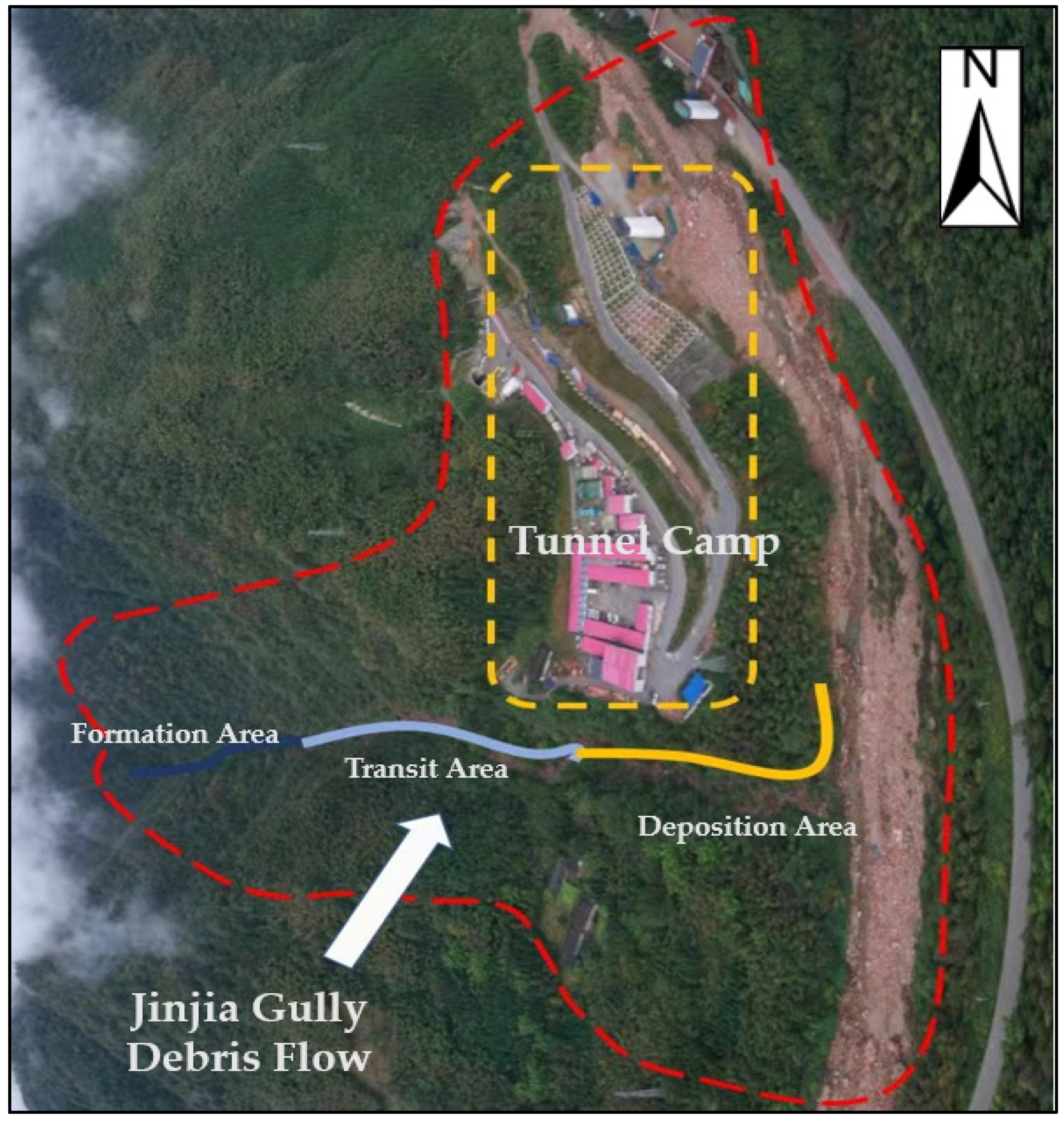
The tunnel camp is located in the southwestern part of Tianquan County, Ya’an City, Sichuan Province. It is situated in the downstream alluvial fan area of Jinjia Gully, within the jurisdiction of Sijing Town. The coordinates of the camp are 102°38′52.14″ N, 29°59′57.22″ E, approximately 18.09 km from Tianquan County town, according to Figure 1. Jinjia Gully watershed is located in the transitional zone between the Chengdu Plain and the western edge of the Panxi Plateau, characterized by tectonic erosion and denudation, forming a high-middle mountainous terrain. The area is often shaped by tectonic erosion, resulting in the formation of valleys. The watershed covers an approximate area of 2.8 km2, with a main channel length of about 2.026 km. The lowest point in the watershed is at the mouth of the gully, with an elevation of 1080 m, and the highest point reaches an elevation of 1778 m, resulting in a relative elevation difference of 698 m. The lower section of the channel exhibits relatively gentle terrain, while steep slopes with variable channel width characterize the upper section. Localized areas along the channel banks contain abundant loose deposits, and the riverbed is extremely rough. Large rocks or accumulations of trees are visible within the channel, indicating certain characteristics of debris flow [21].
Based on regional geological data, the Jinjia Gully watershed is located at the junction of the central part of the large-scale Qinghai–Tibet, Yunnan–Indochina ‘W-shaped’ tectonic system, and the northeast-trending structural belt of the Longmenshan Mountains. The predominant structural trend in this area is northeast, with some additional presence of arcuate and northwest-trending structures. The geological structure of the watershed is complex and diverse, characterized by the development of folds and faults. The rock types in the geological formations are primarily composed of quaternary residual accumulation layers, debris layers, debris flow deposit layers, and channel deposit layers.
The region is a mountainous climate zone influenced by a subtropical monsoon climate, exhibiting mild temperatures, abundant rainfall, and relatively frequent cloudiness with less fog. According to meteorological station data, the annual average temperature occurs in August, reaching 23.8 °C, while the lowest average temperature is observed in January, at only 5.2 °C. The rainy season in this region extends for about half a year, with over 200 rainy days, and a particularly notable rainfall frequency in late summer and early autumn, reaching up to 73%. The annual precipitation ranges from 1158 to 2163 mm, with an average of 1663 mm. One of the major causes of landslide triggering on sandy slopes is heavy rainfall occurrences [22]. Meanwhile, large precipitation is one of the dominant contributing factors to the debris flow events in this region. Moreover, precipitation increases with elevation from east to west, showing an intensified pattern. Therefore, this area is characterized as a typical rainfall-triggered debris flow region, primarily driven by rainfall as the main water source [21].
Human engineering activities within the Jinjia Gully watershed primarily involve slope reduction for housing construction on the alluvial fan at the gully mouth and the construction of the tunnel between Tianquan Station and Dayuxi Station. The topography within this watershed is relatively confined, leading to limited land use options, and there is a widespread occurrence of human activities such as artificial slope cutting and toe excavation [21]. According to historical records and research findings, no debris flow disasters have occurred in the watershed in the past. However, considering factors such as topography, rainfall, and sediment sources, Jinjia Gully possesses all the necessary conditions to trigger debris flow. Therefore, the construction camp located in the alluvial fan area at the gully mouth presents certain safety risks.
3. Debris Flow Hazard Assessment
Modeling was conducted based on the FLO-2D numerical simulation theory and methodology for debris flow movement [23]. The analysis primarily considered three rainfall frequencies (1%, 2%, and 5%), incorporating traditional rainfall–runoff models and the dynamic characteristics of debris flow for hazard assessment. The fundamental principles and specific simulation procedures of the FLO-2D software have been extensively documented in the relevant literature [24,25]; therefore, detailed elaboration is omitted here. Instead, focus is placed on introducing the selection of key parameters and processing relevant data.
3.1. Processing Topographic Data
This study employed unmanned aerial vehicle (UAV) photogrammetry to obtain a high-precision digital elevation model (DEM) of the Jinjia Gully watershed. Subsequently, the DEM was converted into an ASCII file format recognizable by FLO-2D using ArcGIS. Following this, the simulation domain boundaries were delineated, and interpolation calculations for elevation points on the grid were performed. The selection of grid size significantly influences the simulation results and computational accuracy. If the grid is too small, it may pose challenges for the computational hardware; conversely, if the grid is too large, the simulation results may be relatively coarse, making it difficult to accurately reflect the movement trajectory and final accumulation morphology of the debris flow. Considering these requirements, this study partitioned the computational grid in FLO-2D simulation into 1 m × 1 m grids and, based on field survey results, designated the vicinity of the debris flow initiation point as the starting point for numerical simulation.
3.2. Establishing the Debris Flow Discharge Hydrograph
To perform a numerical simulation of debris flow using FLO-2D software (the FLO-2D version is “build 23”), it is necessary to calculate the flow discharge hydrograph of the debris flow. Firstly, based on the “Rainstorm Flood Calculation Manual for Small and Medium-sized Watersheds in Sichuan Province” (1984), Equation (1) is employed to calculate the peak flow discharge under three rainfall frequencies,
where is the maximum peak flow dicharge (m3/s), is the peak runoff coefficient, with values as indicated in Table 1, is the rainfall intensity, representing the maximum 1 h rainfall amount (mm/h), with values as specified in Table 1, is the watershed concentration time (h), with values as given in Table 1, is the rainfall formula exponent, with values as listed in Table 1, and is the watershed drainage area (km2), with a value of 2.8.
Referring to Appendix A of the “Specification of geological investigation for debris flow stabilization” (DZ/T0220-2006), Equation (2) is employed to calculate the peak flow discharge of debris flow under three rainfall frequencies,
where is the peak flow discharge of debris flow (m3/s), is the sand correction coefficient, and are obtained from on-site slurry mixing experiments, is the density of debris flow (t/m3), the values can be referred to in Table 1, is the specific gravity of solid material in debris flow (t/m3), with a value of 2.65, is the density of clear water (t/m3), and its value is 1, is the blockage coefficient of debris flow, according to the characteristics of the channel and material composition of the debris flow as per the “Specification of geological investigation for debris flow stabilization” (DZ/T0220-2006) Table A1, the Jinjia Gully channel is relatively straight, with a uniform width in the segments, and there are few steep steps and narrow constrictions. Additionally, the formation area of the debris flow is not highly concentrated, and the situation of riverbed blockage is generally moderate, with the flow exhibiting a viscous slurry to thin porridge state. Based on these characteristics, the recommended value from the table is taken as 2.0. The results of rainfall peak flow and debris flow peak flow calculations under different rainfall frequencies at the watershed cross-section are shown in Table 2.
According to the method proposed by Zou Qiang [26], the calculation of the duration of debris flow events can based on the watershed area, as shown in Equation (4),
where is the duration of debris flow (s), is the watershed area (km2). is 2.8 km2; can be assigned a value of 1800 s. Based on the above data, this study employs the simplified pentagon generalization method to obtain the debris flow discharge hydrograph [27], as shown in Figure 2.
3.3. Selecting Relevant Parameters for Debris Flow Simulation
Unlike landslides [28], the main factors affecting the triggering and mechanical process of debris flow include Manning’s coefficient (), volume concentration (), laminar flow resistance coefficient (), viscous coefficient (), and yield stress coefficient (). The selection of these relevant parameters should be determined through field investigations and on-site analysis. Additionally, the parameter selection rules outlined in the FLO-2D technical manual should be considered [29]. The final values are presented in Table 3.
3.4. Simulating Debris Flow and Zoning for Hazard Assessment
Inputting the aforementioned discharge and relevant parameters into the FLO-2D model for simulation and considering the actual conditions of debris flow in Jinjia Gully, the appropriate indicators are selected from the simulation results to characterize the level of hazard in different areas within the impact zone of the debris flow [8]. This paper draws on the comprehensive debris flow hazard model proposed by Fiebiger [30], as seen in Equation (5),
where is the hazard of debris flow, is the flow velocity (m/s), is the low depth (m), and the value of is 9.8 (m2/s).
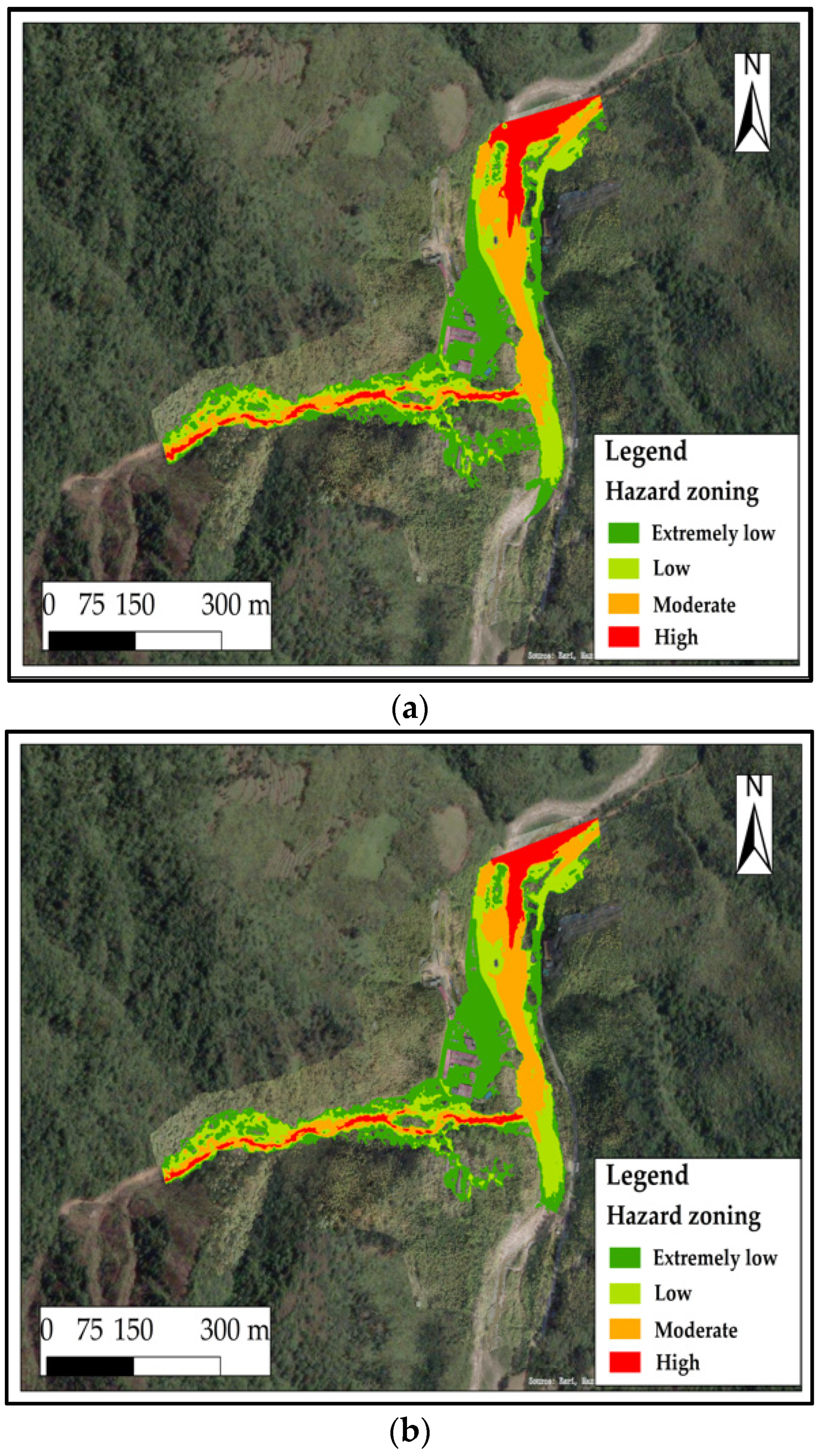
This study utilizes the model to perform calculations on the numerical simulation results of debris flow in Jinjia Gully. Subsequently, using the natural break method in ArcGIS, the hazard is classified, resulting in hazard zoning maps for the area affected by debris flow after outbreaks under three rainfall frequencies, as shown in Figure 3.
3.5. Verifying the Simulation Results of Debris Flow
By comparing numerical simulations and computational results, validation is conducted on the total solid material expelled during a debris flow to assess the accuracy and reliability of the numerical simulation outcomes. According to the “Specification of geological investigation for debris flow stabilization” (DZ/T0220-2006), the total amount of solid material expelled during a debris flow can be calculated according to Equation (6),
where is the total amount of solid material expelled during a debris flow (m3), is the total volume of flow during a debris flow (m3), is the duration of the debris flow (s), and is the flow coefficient, and its value varies with the watershed area (). When , , with the other parameters having the same meanings as mentioned earlier.
The above formula can calculate the total amount of solid material expelled during a debris flow under three different rainfall frequencies. In the FLO-2D numerical simulation, the total solid material expelled during a debris flow can be obtained by multiplying the flow depth of each computational unit by its corresponding area in ArcGIS and then summing the results. The specific calculation results and numerical simulation outcomes are shown in Table 4.
As evident from Table 4, the simulation results under three different scenarios closely align with the calculated results, with the error falling within an acceptable range, meeting the precision requirements. Consequently, the numerical simulation conducted in this study exhibits a certain level of reliability. Additionally, it is noteworthy that the calculated results tend to be higher than the simulated results. This is because the simulation results only encompass the total expelled solid material below the outflow point, excluding the solid material above it [8]. However, the solid material above the outflow point constitutes only a small fraction of the expelled material. Therefore, the magnitude of this error is within a reasonably acceptable range.
The simulation results indicate that, under rainfall frequencies of p = 5% and p = 2%, the hazardous area within the debris flow impact zone is relatively small. However, under a rainfall frequency of p = 1%, the watershed’s hazardous area rapidly expands, with significant coverage in the moderate- to high-risk zones. Individuals and structures within the channel sides and distant areas of the debris fan are generally exposed to substantial threats.
4. Vulnerability Assessment of Large-Scale Temporary Works—Indicator Factor
Large-scale temporary works (hereinafter referred to as “LT works”) refer to engineering projects of significant scale, limited duration, and non-permanent nature. The construction period for LT works typically spans several months, with the scale varying depending on the type of project. These works are often rapidly erected within a specific timeframe to ensure the smooth progress of the project and are completely dismantled or removed upon completion of the tasks. Due to their temporary nature, LT works often feature simplified structures and designs, utilizing temporary and cost-effective materials. The construction elements are generally located in flat debris flow deposition fan areas or scattered along the railway corridors. Consequently, there is a higher likelihood of being impacted by debris flow.
LT works vulnerability refers to the degree of losses that occur in LT works under the influence of geological disasters. It reflects the resilience, response, and recovery capabilities of these works when affected by disasters and is quantitatively expressed as vulnerability ().
4.1. Selecting Evaluation Indicators
Focused on LT works, based on domestic and international literature reviews and field visits and considering the characteristics of debris flow disasters and natural environmental conditions, a vulnerability assessment system was ultimately constructed. This system revolves around the functions and application requirements of construction camps and other building complexes, focusing on three dimensions: engineering type, structural characteristics, and construction quality.
4.2. Determining Indicator Weights
In accordance with the requirements of the Analytic Hierarchy Process (AHP), a “Large-scale temporary works Vulnerability Assessment Indicator Survey Questionnaire” was designed. The questionnaire contains information on primary and secondary assessment indicators. It is intended for scoring by researchers, academics from universities, and graduate students with a background in geological disasters.
For each level of indicators, pairwise comparisons were conducted using a scale from 1 to 9 to express the relative importance of the indicators. The sorting results were utilized to construct a judgment matrix using the AHP software yaahp10.1, and a consistency check was performed on the matrix [31]. The results were considered acceptable if the consistency ratio was less than 0.1. Finally, the weight coefficients for each indicator were calculated based on the eigenvector corresponding to the maximum eigenvalue of the judgment matrix. The detailed results are presented in Table 5 and Table 6.
4.3. Establishing Vulnerability Functions and Vulnerability Classification
An analysis based on Table 5 and Table 6 reveals that the vulnerability of each individual LT work can be calculated using Equation (8),
where , , and are the weights corresponding to the secondary indicators. In Table 6, the value of ranges from 1 to 2, and in Table 5, the value of ranges from 1 to 17; the value of in Table 6 ranges from 3 to 4, and in Table 5, the value of ranges from 18 to 20; the value of in Table 6 ranges from 5 to 7, and in Table 5, the value of ranges from 21 to 23. is the score assigned to the types corresponding to the secondary indicators, and the selection should be based on a comprehensive consideration of questionnaire details and actual survey conditions.
Combining field investigations with remote sensing imagery, interpret each temporary work in the study area individually (refer to Figure 4). Then, follow the above model for calculations. After calculations, normalize the vulnerability value to (see Table 7 and Table 8). Utilizing the ArcGIS platform and employing the natural breaks method, the LT works in the study area were classified into four levels: high, moderate, low, and extremely low vulnerability, as shown in Table 9.
5. Analysis of Shielding Effects—Modified Indicator Factor Assessment Method
The indicator factor assessment method mentioned above only considers the vulnerability of individual LT works. However, the densely distributed building complexes in the construction camps of LT works can impact the debris flow field, thereby affecting the impact force on buildings at different locations. The shielding effect between buildings is evident.
Therefore, based on the physical model experiment of the spatial distribution of debris flow impact force, this study aims to quantify the impact of the shielding effect of building complexes on debris flow movement. The objective is to determine the relationship between the spatial distribution and relative positions of buildings and building damage. This will lead to modifying the vulnerability assessment model obtained from the indicator mentioned above method. The ultimate goal is to establish a vulnerability assessment method that reflects the distribution characteristics of construction camps.
5.1. Experimental Design and Setup
As shown in Figure 5, this experiment simulated the debris flow fan area in a rectangular test area of 2.5 m × 1.8 m. The bottom plate of this area was perforated with a spacing of 12.5 cm × 10 cm, forming a grid of 24 × 17 with a grid size of 10 cm × 10 cm. The red X-axis in the figure represents the positive flow direction, and the Y-axis represents the transverse direction. X1 is used to denote the vertex of the debris flow fan. The dimensions of the experimental tank are 1 m (length) × 0.2 m (width) × 0.2 m (height), with a slope of 12°. The top of the tank is fixed with a feeding pool with a maximum volume of 80 L. In order to better simulate the process of building damage caused by debris flow impact in the fan area, square impact resistance-type sensors (cubes of 2 cm × 2 cm × 2 cm) were used in this experiment. The impact range of these sensors is 0~20 kPa, and the sampling frequency of the data acquisition system is 1000 Hz.
The experimental design is divided into two parts: the clear water impact experiment, used for instrument detection and as a control experiment, and the impact experiments of debris flows with three different bulk densities. A total of 100 impact force measurement experiments were conducted. This study adopted the undisturbed soil proportion of debris flow from the demonstration site, Jiangjia Gully, to make the experimental results more universal.
The experimental approach is divided into the following two parts:
(1) Flow direction (distance): The impact pressure at different locations within the flow direction was measured at intervals of 12.5 cm in the range of 0~75 cm to analyze the distribution of impact pressure along the flow path (Figure 6). Subsequently, a pressure sensor was fixed at the outlet of the debris flow fan, specifically at . Using the same distances as mentioned above, the impact pressure distribution at different locations within the flow direction was sequentially measured. This was performed to analyze the variation in impact force after the building was obstructed.
(2) Strike direction (angle): In the preliminary experiment stage, it was observed from the flow states of fluids with different densities that the debris flow distributed on the debris flow fan board generally reached the maximum flow width at , indicating that the flow width gradually decreases after exceeding . Therefore, in the second part, sensors are arranged along the strike direction at of the debris flow fan with intervals of 10 cm (Figure 7). The sensing surface of the sensors is not facing directly towards the incoming direction of the debris flow but forms an increasingly larger angle with the X-axis. Similarly, a pressure sensor is fixed at the outlet of the debris flow fan at as an obstruction. Following the aforementioned intervals, the impact pressure distribution at different angles is measured to analyze the changes in strike force after the obstruction is introduced.
5.2. Data Processing and Results
This paper employs wavelet analysis to denoise the signals of debris flow impact force [32,33]. The following presents the processed measurement data of sensors for each experimental group, with the mean impact force within a stable period of 0.5 s after selecting the peak (Appendix A).
5.3. Analysis of Shielding Effects
(1) Flow direction: Figure 8a shows the experimentally measured variation of impact pressure along the path under unobstructed conditions for four different bulk density fluids, ranging from clear water with a density of 1.0 g/cm3 to debris flow with a density of 2.0 g/cm3. The impact pressure experienced by the sensor at different locations within the debris flow fan varied significantly, decreasing gradually along the flow path. is the normalized impact pressure measured at different locations (normalized to the impact pressure at location ). is the spatial flow direction positions for the buildings, is the distance from the building (sensor) to the debris flow fan area , and is the building (sensor) size. The variation of impact pressure along the path for the four different bulk density fluids can be fitted with a polynomial function through indoor flume experiments (as shown in Equation (9)). Furthermore, from Figure 5a, it is evident that when > 37.5, the impact pressure decreases to less than 10% of the maximum value. The values of the four bulk density fluid coefficient types in the equation are listed in Table 10.
The effect of the front building on the impact pressure of the rear one is shown in Figure 8b. is the impact pressure ratio with shielding; is the distance between the two buildings. When < 37.5, the impact force reduction decreases with the building spacing increase. When > 37.5, the shielding effect becomes negligible. The ratio of impact force of the rear building with and without the shielding effect is Equation (10); the coefficients are shown in Table 11.
(2) Strike direction: Figure 9 has the angle in radians () as the horizontal axis, with the same meaning as described above for the vertical axis. It can be observed that when < 0.674 radians, the decrease in impact force diminishes as the angle between the front and rear buildings increases. However, when > 0.674 radians, the influence of the front building on the rear building is almost negligible, and the shielding effect can be disregarded. The specific fitting function is shown in Equation (11), and the coefficients are listed in Table 12.
(3) Combining distance and angle: When there is a shielding effect between buildings, the significant reduction in impact force will greatly affect the vulnerability assessment results obtained using the aforementioned index method. Therefore, it is necessary to combine the two (see Equation (12)), re-adjust the vulnerability values to obtain , and finally normalize them using the ArcGIS platform to obtain , thus enabling a more accurate vulnerability assessment.
where and are the shielding factors for the flow and strike direction, respectively, . and are the average values of the three bulk density coefficients for debris flows.
5.4. Case Study
This paper integrates remote sensing interpretation and field survey findings to propose that Building No. 10 located at the apex of the alluvial fan at the mouth of the gully be considered as an obstruction at position in the flume experiment. Considering the complexity of the actual terrain and building structure, Building No. 10 is simplified into a cubic model measuring 6 m × 6 m × 6 m for ease of calculation (to ensure consistency with the experiment, other buildings are also simplified to this model), i.e., = 6 m (with a depth of approximately 6 m, and its upstream face facing the debris flow coincides with its depth face). Therefore, according to the formula from the previous context, when > 37.5 × = 225 m, the shielding effect can be negligible.
From the extent of debris flow inundation and Figure 10, it can be inferred that the distribution of LT works in the study area can be classified into the following two categories:
(1) The following 17 buildings are not within the numerical simulation inundation range of the debris flow and are not considered for shielding effects (outlined by the black line in the detailed map of the construction camp): Buildings numbered 19, 20, 21, 22, 23, 24, 25, 34, 36, 37, 42, 43, 44, 45, 46, 47, and 48. Their vulnerability values remain unchanged.
(2) The remaining 31 buildings are within the inundation range of the debris flow and may require consideration for shielding effects. The analysis is as follows:
1) When = 0, the buildings should be positioned along the Y-axis in the figure. From Figure 8, it is evident that there is no need to exclude buildings without shielding effects (except for Building No. 10).
2) When > 225 m, at this point, = 1. This can further be divided into the following situations:
① When > 0.674 rad, at this point, = 1. It can be seen that the four buildings numbered 38, 39, 40, and 41 meet this condition; therefore, their vulnerability values remain unchanged.
② When = 0 rad, the buildings should be positioned along the X-axis in the figure, considering only the downstream shielding effect, meaning = . From the figure, it can be observed that there are no buildings in this situation.
③ When 0 < 0.674 rad, there are no buildings that meet this condition.
3) When 0 < 225 m, divided into the following situations:
① When > 0.674 rad, at this point, = 1. From the figure, it can be observed that the 18 buildings numbered 5, 11, 12, 13, 14, 15, 16, 17, 18, 26, 27, 28, 29, 30, 31, 32, 33, and 35 meet this condition. Additionally, through a combination of field surveys and distance measurement techniques on the ArcGIS platform, the distance between these buildings within the camp and Building No. 10 has been determined. Using Formulas (10) and (12), as well as referencing Table 11, the vulnerability values for these buildings under shielding effects have been calculated (Table 13).
② When = 0 rad, the buildings should be positioned along the X-axis in the figure, considering only the downstream shielding effect. From the figure, it can be inferred that buildings numbered 1 and 2 meet this condition. Following the previously mentioned method, their adjusted vulnerability values have been calculated (Table 14).
③ When 0 < 0.674 rad, at this point, both distance and angle shielding effects should be considered. From the figure, it can be determined that buildings numbered 3, 4, 6, 7, 8, and 9 meet this condition. Using Formulas (10)–(12), as well as referencing Table 11 and Table 12, the vulnerability values for these buildings under shielding effects have been calculated (see Table 15).
Based on the above analysis, the vulnerability zoning map of LT works in the study area before and after correction for the experiment is as follows:
(1) Considering the shielding effects, the vulnerability ratings of buildings in construction camps numbered 3 and 7 have changed from low to extremely low. Buildings numbered 2, 16, 29, 30, and 31 have changed from moderate to low vulnerability ratings. Buildings numbered 11, 12, 13, 14, 17, and 18 have changed from high to low vulnerability ratings. Building No. 9, being close to the X-axis, shows the most noticeable change in vulnerability rating, directly shifting from high to extremely low vulnerability. The vulnerability ratings of the other 12 buildings affected by the shielding effects have remained unchanged.
(2) From Figure 11a, it can be observed that the number of buildings in the study area classified as extremely low, low, moderate, and high vulnerability levels is 8, 12, 8, and 20, respectively, with buildings classified as moderate to high vulnerability levels accounting for 58.33% of the total buildings. From Figure 11b, it can be seen that after experimental adjustments, the number of buildings in the study area classified as extremely low, low, moderate, and high vulnerability levels is 11, 21, 3, and 13, respectively, with buildings classified as moderate to high vulnerability levels accounting for 33.33% of the total buildings. Due to the presence of actual shielding effects, the overall vulnerability of the buildings in the study area shifted from moderate to high to low and extremely low levels. Notably, the accesses and bridges were not considered for shielding effects. The lengths of these accesses and bridges classified as extremely low, low, moderate, and high vulnerability levels are 1401.15 m, 0 m, 123.78 m, and 352.94 m, respectively, with a significant proportion of accesses and bridges classified as extremely low and low vulnerability levels, reaching 74.61%. Therefore, the overall vulnerability of the accesses and bridges in the study area is relatively low.
6. Risk Assessment of Large-Scale Temporary Works (p = 5%)
The debris flow risk assessment is the product of hazard (H) and vulnerability (V). It involves quantitative analysis and evaluation of the likelihood of different-intensity geological hazards occurring in risk-prone areas and the potential disaster losses they may cause [34]. This is a highly practical and important research topic. Table 16 provides a detailed description of different risk levels and their characteristics for large-scale temporary works. The superimposed calculation yields the risk zoning results for the debris flow in the tunnel camp, which occurs once every twenty years, as shown in Figure 12.
The results indicate that the percentages of assessment units with building risk levels classified as extremely low, low, moderate, and high under a rainfall frequency of 5% are 75%, 16.67%, 8.33%, and 0%, respectively. For access risk levels, the percentages of assessment units classified as extremely low, low, moderate, and high are 66.99%, 24.08%, 8.93%, and 0% of the total assessment units, respectively.
It can be observed that a significant proportion of LT works are situated in areas of extremely low and low risk, indicating that the study area is at a low risk level. This result aligns well with the actual situation observed during field surveys and reflects the expected future development trends. It also indicates that the risk assessment of LT works in the study area is determined by both natural and social factors. Therefore, the reliability of the assessment results is relatively high.
7. Discussion and Conclusions
The FLO-2D software itself is primarily a numerical computation software for simulating flood and debris flow disasters [35]. The model is equipped with binary limitations and six assumptions [36]. Therefore, numerical simulations and hazard assessments inevitably deviate from actual conditions. The experimental correction part of this study regarding the shielding effect assumes that throughout the entire process of a debris flow disaster, the preceding buildings will not collapse and block the debris flow. At the same time, this paper does not consider the progressive collapse of building clusters and its impact on the shielding effect.
The model does not consider factors affecting flow velocity and impact force. One is the slope of the debris fan, which is related to the size of debris in the debris flow and the sediment concentration [37]. Although the slope of most debris fans is between 0 and 5°, its influence on the deposition of debris flow material and flow velocity is insignificant. Another factor is turbulent characteristics (e.g., solid/liquid ratio and viscosity), which directly affect the impact force and ultimately influence the magnitude of the shielding effect. The debris flow density used in the experiments in this paper is between 1.8 and 2.0 g/cm3. When the debris flow density is less than 1.8 g/cm3, the impact force may decrease, leading to a possible overestimation of the vulnerability of buildings in the current assessment model. Therefore, subsequent research needs to explore the impact of the shielding effect using debris flows composed of different solid/liquid ratios and particle size distributions.
This paper employs a combined approach of numerical simulation and experimental research. It evaluates the debris flow disaster risk on a single gully scale in the Jinjia Gully of Tianquan County, using LT works on debris fans as assessment units. As an example, the assessment results are based on rainfall frequencies occurring once every twenty years. The simulation of debris flows under different rainfall frequencies was conducted, and due to the reasonable selection of parameters, the simulation results were satisfactory. Upon validation, the simulated results closely matched the calculated results, indicating a high level of reliability in this simulation.
This paper focuses on LT works located on debris fans and proposes a novel vulnerability assessment model. This model not only comprehensively considers the characteristics of the structure and materials of LT works but also considers the shielding effect’s influence when assessing the vulnerability of a group of buildings. As a result, it can provide new approaches for future studies of the interaction mechanism between debris flow disasters and LT works.
Future research can address the limitations of the assessment methods above and continue to comprehensively and systematically document various types of debris flow disasters post-event. This will enable the development of multiple assessment models that are more applicable and comprehensive.
Author Contributions
Y.W. contributed to the conceptualization, methodology, formal analysis, resources, software, investigation, visualization, and writing—original draft, review, and editing. Y.L. contributed to the conceptualization, methodology, formal analysis, resources, software, editing and supervision. H.G. contributed to the methodology, resources, editing and supervision. All authors have read and agreed to the published version of the manuscript.
Funding
This research received no external funding.
Data Availability Statement
Data will be made available on request.
Acknowledgments
This work was supported National Key Research and Development Program of China (grant no. 2023YFC3008303) and National Natural Science Foundation of China (grant no. 41941017) and IMHE Program (grant no. IMHE-ZDRW-02).
Conflicts of Interest
The authors declare no conflicts of interest.
Appendix A
The appendix is the data processing results of debris flow impact force.

Table A1.
Data processing results of debris flow impact force (flow directions).
| ID | Experimental Conditions | Measured Sensors | Impact Force Value (kPa) | |
|---|---|---|---|---|
| 1 | 1.0 | X1 | X1 | 5.94 |
| 2 | 1.0 | X2 unshielding | X2 | 5.21 |
| 3 | 1.0 | X2 shielding | X2 | 1.62 |
| 4 | 1.0 | X3 unshielding | X3 | 4.69 |
| 5 | 1.0 | X3 shielding | X3 | 2.52 |
| 6 | 1.0 | X4 unshielding | X4 | 3.39 |
| 7 | 1.0 | X4 shielding | X4 | 2.69 |
| 8 | 1.0 | X5 unshielding | X5 | 3.43 |
| 9 | 1.0 | X5 shielding | X5 | 2.99 |
| 10 | 1.0 | X6 unshielding | X6 | 1.69 |
| 11 | 1.0 | X6 shielding | X6 | 1.61 |
| 12 | 1.0 | X7 unshielding | X7 | 0.97 |
| 13 | 1.0 | X7 shielding | X7 | 0.96 |
| 14 | 1.8 | X1 | X1 | 7.74 |
| 15 | 1.8 | X2 unshielding | X2 | 6.53 |
| 16 | 1.8 | X2 shielding | X2 | 1.96 |
| 17 | 1.8 | X3 unshielding | X3 | 5.89 |
| 18 | 1.8 | X3 shielding | X3 | 3.24 |
| 19 | 1.8 | X4 unshielding | X4 | 4.49 |
| 20 | 1.8 | X4 shielding | X4 | 3.02 |
| 21 | 1.8 | X5 unshielding | X5 | 3.33 |
| 22 | 1.8 | X5 shielding | X5 | 2.94 |
| 23 | 1.8 | X6 unshielding | X6 | 2.32 |
| 24 | 1.8 | X6 shielding | X6 | 2.19 |
| 25 | 1.8 | X7 unshielding | X7 | 1.02 |
| 26 | 1.8 | X7 shielding | X7 | 0.99 |
| 27 | 1.9 | X1 | X1 | 9.96 |
| 28 | 1.9 | X2 unshielding | X2 | 8.29 |
| 29 | 1.9 | X2 shielding | X2 | 2.51 |
| 30 | 1.9 | X3 unshielding | X3 | 7.47 |
| 31 | 1.9 | X3 shielding | X3 | 5.08 |
| 32 | 1.9 | X4 unshielding | X4 | 5.78 |
| 33 | 1.9 | X4 shielding | X4 | 4.63 |
| 34 | 1.9 | X5 unshielding | X5 | 3.49 |
| 35 | 1.9 | X5 shielding | X5 | 3.12 |
| 36 | 1.9 | X6 unshielding | X6 | 2.99 |
| 37 | 1.9 | X6 shielding | X6 | 2.45 |
| 38 | 1.9 | X7 unshielding | X7 | 1.27 |
| 39 | 1.9 | X7 shielding | X7 | 1.25 |
| 40 | 2.0 | X1 | X1 | 11.52 |
| 41 | 2.0 | X2 unshielding | X2 | 11.06 |
| 42 | 2.0 | X2 shielding | X2 | 3.01 |
| 43 | 2.0 | X3 unshielding | X3 | 9.91 |
| 44 | 2.0 | X3 shielding | X3 | 4.16 |
| 45 | 2.0 | X4 unshielding | X4 | 7.49 |
| 46 | 2.0 | X4 shielding | X4 | 5.25 |
| 47 | 2.0 | X5 unshielding | X5 | 5.65 |
| 48 | 2.0 | X5 shielding | X5 | 5.01 |
| 49 | 2.0 | X6 unshielding | X6 | 3.46 |
| 50 | 2.0 | X6 shielding | X6 | 3.29 |
| 51 | 2.0 | X7 unshielding | X7 | 2.07 |
| 52 | 2.0 | X7 shielding | X7 | 2.05 |
Table A2.
Data processing results of debris flow impact force (strike directions).
| ID | Experimental Conditions | Measured Sensors | Impact Force Value (kPa) | |
|---|---|---|---|---|
| 53 | 1.0 | Y2 unshielding | Y2 | 1.14 |
| 54 | 1.0 | Y2 shielding | Y2 | 0.35 |
| 55 | 1.0 | Y3 unshielding | Y3 | 1.69 |
| 56 | 1.0 | Y3 shielding | Y3 | 0.93 |
| 57 | 1.0 | Y4 unshielding | Y4 | 0.92 |
| 58 | 1.0 | Y4 shielding | Y4 | 0.74 |
| 59 | 1.0 | Y5 unshielding | Y5 | 0.75 |
| 60 | 1.0 | Y5 shielding | Y5 | 0.62 |
| 61 | 1.0 | Y6 unshielding | Y6 | 0.24 |
| 62 | 1.0 | Y6 shielding | Y6 | 0.23 |
| 63 | 1.0 | Y7 unshielding | Y7 | 0.09 |
| 64 | 1.0 | Y7 shielding | Y7 | 0.09 |
| 65 | 1.8 | Y2 unshielding | Y2 | 2.03 |
| 66 | 1.8 | Y2 shielding | Y2 | 0.34 |
| 67 | 1.8 | Y3 unshielding | Y3 | 2.97 |
| 68 | 1.8 | Y3 shielding | Y3 | 1.43 |
| 69 | 1.8 | Y4 unshielding | Y4 | 1.59 |
| 70 | 1.8 | Y4 shielding | Y4 | 0.97 |
| 71 | 1.8 | Y5 unshielding | Y5 | 1.06 |
| 72 | 1.8 | Y5 shielding | Y5 | 0.85 |
| 73 | 1.8 | Y6 unshielding | Y6 | 0.62 |
| 74 | 1.8 | Y6 shielding | Y6 | 0.56 |
| 75 | 1.8 | Y7 unshielding | Y7 | 0.23 |
| 76 | 1.8 | Y7 shielding | Y7 | 0.21 |
| 77 | 1.9 | Y2 unshielding | Y2 | 2.29 |
| 78 | 1.9 | Y2 shielding | Y2 | 0.45 |
| 79 | 1.9 | Y3 unshielding | Y3 | 3.16 |
| 80 | 1.9 | Y3 shielding | Y3 | 1.83 |
| 81 | 1.9 | Y4 unshielding | Y4 | 1.77 |
| 82 | 1.9 | Y4 shielding | Y4 | 1.24 |
| 83 | 1.9 | Y5 unshielding | Y5 | 1.21 |
| 84 | 1.9 | Y5 shielding | Y5 | 0.98 |
| 85 | 1.9 | Y6 unshielding | Y6 | 0.69 |
| 86 | 1.9 | Y6 shielding | Y6 | 0.53 |
| 87 | 1.9 | Y7 unshielding | Y7 | 0.12 |
| 88 | 1.9 | Y7 shielding | Y7 | 0.11 |
| 89 | 2.0 | Y2 unshielding | Y2 | 2.91 |
| 90 | 2.0 | Y2 shielding | Y2 | 0.88 |
| 91 | 2.0 | Y3 unshielding | Y3 | 3.58 |
| 92 | 2.0 | Y3 shielding | Y3 | 1.79 |
| 93 | 2.0 | Y4 unshielding | Y4 | 2.09 |
| 94 | 2.0 | Y4 shielding | Y4 | 1.27 |
| 95 | 2.0 | Y5 unshielding | Y5 | 1.54 |
| 96 | 2.0 | Y5 shielding | Y5 | 0.82 |
| 97 | 2.0 | Y6 unshielding | Y6 | 1.07 |
| 98 | 2.0 | Y6 shielding | Y6 | 0.94 |
| 99 | 2.0 | Y7 unshielding | Y7 | 0.26 |
| 100 | 2.0 | Y7 shielding | Y7 | 0.25 |
References
- Lambe, T.W.; Whitman, R. Soil Mechanics; CHAPTER on Soil Stability with Flow; MIT: Cambridge, MA, USA; Wiley: New York, NY, USA, 1969. [Google Scholar]
- Cui, P.; Zou, Q. Theory and methods of risk assessment and risk management of mountain flood and debris flow. Geograph 2016, 2, 4. [Google Scholar]
- Peng, J.B.; Cui, P.; Zhuang, J.Q. Challenges to engineering geology of Sichuan-Tibet railway. Chin. J. Rock Mech. Eng. 2020, 39, 2377–2389. [Google Scholar]
- Lu, C.; Cai, C. Challenges and countermeasures for construction safety during the Sichuan–Tibet railway project. Engineering 2019, 5, 833–838. [Google Scholar] [CrossRef]
- Zou, Q.; Jiang, L.; You, Y.; Wang, D.; Jiang, H.; Zhang, G. Information Management System for Mountain Hazards along Sichuan-Tibet Railway. J. Yangtze River Sci. Res. Inst. 2020, 37, 177. [Google Scholar]
- Wei, R.; Zeng, Q.; Davies, T.; Yuan, G.; Wang, K.; Xue, X.; Yin, Q. Geohazard cascade and mechanism of large debris flows in Tianmo gully, SE Tibetan Plateau and implications to hazard monitoring. Eng. Geol. 2018, 233, 172–182. [Google Scholar] [CrossRef]
- Cui, P.; Ge, Y.; Li, S.; Li, Z.; Xu, X.; Zhou, G.G.; Chen, H.; Wang, H.; Lei, Y.; Zhou, L.; et al. Scientific challenges in disaster risk reduction for the Sichuan–Tibet Railway. Eng. Geology. 2022, 309, 106837. [Google Scholar] [CrossRef]
- Li, B.X.; Cai, Q.; Song, J.; Chen, L.; Liu, J.-K. Risk assessment of debris flow disasters based on FLO-2D: A case study of the Maiduogou debris flow. J. Nat. Disasters 2022, 31, 256. [Google Scholar]
- Jia, T.; Tang, C.; Wang, N. Zoning method and application of debris flow hazard based on FLO-2D and momentum model. Hydroelectr. Energy Sci. 2015, 33, 152–155. [Google Scholar]
- Zhang, P.; Ma, J.; Shu, H.; Wang, G. Numerical simulation of debris flow movement and erosion-sedimentation based on the FLO-2D model. J. Lanzhou Univ. Nat. Sci. 2014, 50, 363–368. [Google Scholar]
- Lin, J.-Y.; Yang, M.-D.; Lin, B.-R.; Lin, P.-S. Risk assessment of debris flows in Songhe Stream, Taiwan. Eng. Geol. 2011, 123, 100–112. [Google Scholar] [CrossRef]
- Eidsvig, U.; Papathoma-Köhle, M.; Du, J.; Glade, T.; Vangelsten, B. Quantification of model uncertainty in debris flow vulnerability assessment. Eng. Geol. 2014, 181, 15–26. [Google Scholar] [CrossRef]
- Papathoma-Köhle, M.; Keiler, M.; Totschnig, R.; Glade, T. Improvement of vulnerability curves using data from extreme events: Debris flow event in South Tyrol. Nat. Hazards 2012, 64, 2083–2105. [Google Scholar] [CrossRef]
- Birkmann, J.; Cardona, O.D.; Carreño, M.L.; Barbat, A.H.; Pelling, M.; Schneiderbauer, S.; Kienberger, S.; Keiler, M.; Alexander, D.; Zeil, P.; et al. Framing vulnerability, risk and societal responses: The MOVE framework. Nat. Hazards 2013, 67, 193–211. [Google Scholar] [CrossRef]
- Apel, H.; Aronica, G.T.; Kreibich, H.; Thieken, A.H. Flood risk analyses—How detailed do we need to be. Nat. Hazards 2009, 49, 79–98. [Google Scholar] [CrossRef]
- Totschnig, R.; Sedlacek, W.; Fuchs, S. A quantitative vulnerability function for fluvial sediment transport. Nat. Hazards 2011, 58, 681–703. [Google Scholar] [CrossRef]
- Papathoma-Köhle, M.; Gems, B.; Sturm, M.; Fuchs, S. Matrices, curves and indicators: A review of approaches to assess physical vulnerability to debris flows. Earth-Sci. Rev. 2017, 171, 272–288. [Google Scholar] [CrossRef]
- Du, Y. Construction of construction camps in permafrost areas of the Qinghai-Tibet Plateau. Railw. Constr. Technol. 2003, z1, 150–152. [Google Scholar]
- Guo, L.B.; Wang, J.G.; Guo, Y.X. Geological disaster hazards of temporary construction camps in high-altitude Tibetan areas. Yunnan Hydropower 2019, 35, 20–21. [Google Scholar]
- Zhao, J.; Li, Z.; Li, R.; Wei, Q.; Yin, H.; Hu, H. Research on key technical issues in the construction of railway construction camps in rugged mountainous areas. China Railw. 2021. [Google Scholar] [CrossRef]
- Xu, Z.X.; Yuan, D.; Liu, Z.J.; Liu, J.F.; You, Y. Development characteristics and risk analysis of debris flow in Songjiagou along the Sichuan-Tibet Railway. J. Yangtze River Sci. Res. Inst. 2020, 37, 165. [Google Scholar]
- Di, B.; Stamatopoulos, C.A.; Stamatopoulos, A.C.; Liu, E.; Balla, L. Proposal, application and partial validation of a simplified expression evaluating the stability of sandy slopes under rainfall conditions. Geomorphology 2021, 395, 107966. [Google Scholar] [CrossRef]
- Gong, K.; Yang, T.; Xia, C.H.; Yang, Y. Risk assessment of debris flow based on FLO-2D: A case study of Cutougou in Mianzili Township, Wenchuan County, Sichuan Province. J. Water Resour. Water Eng. 2017, 28, 134–138. [Google Scholar]
- Zhang, F.X.; Zhang, L.Q.; Zhou, J.; Wang, S. Risk analysis of debris flow in Ruoru Village, Tibet based on FLO-2D. J. Water Resour. Water Eng. 2019, 30, 95–102. [Google Scholar]
- Xu, H.L. Research on Prediction of Debris Flow Runoff Scale in Steep Gullies Based on FLO-2D; Chengdu University of Technology: Chengdu, China, 2018. [Google Scholar]
- Zou, Q.; Cui, P.; Jiang, H.; Wang, J.; Li, C.; Zhou, B. Analysis of regional river blocking by debris flows in response to climate change. Sci. Total Environ. 2020, 741, 140262. [Google Scholar] [CrossRef] [PubMed]
- Hu, G.B. Analytical calculation of flood routing with pentagonal flood hydrograph. Jiangxi Hydraul. Sci. Technol. 1993, 19, 198–201. [Google Scholar]
- Take, W.A.; Bolton, M.D.; Wong, P.C.P.; Yeung, F.J. Evaluation of landslide triggering mechanisms in model fill slopes. Landslides 2004, 1, 173–184. [Google Scholar] [CrossRef]
- O’Brien, J.S.; Garcia, R. FLO-2D Reference Manual. 2009, p. 595. Available online: www.flo-2d.com (accessed on 10 March 2024).
- Fiebiger, G. The Estimation of the Hazard Potency of Debris Flows and The Step to Step Method. In Environmental Forest Science, Proceedings of the IUFRO Division 8 Conference Environmental Forest Science, Kyoto, Japan, 19–23 October 1998; Springer: Amsterdam, The Netherlands, 1998; pp. 529–540. [Google Scholar]
- Zhang, Z.Y.; Liu, Q.; Wang, G.; Xu, Z.W. Research on health assessment of Fenghe River based on AHP-fuzzy mathematical model and item-by-item evaluation method. Pearl River 2023, 44, 9. [Google Scholar]
- Hu, K.; Wei, F.; Li, Y. Real-time measurement and preliminary analysis of debris-flow impact force at Jiangjia Ravine, China. Earth Surf. Process. Landf. 2011, 36, 1268–1278. [Google Scholar] [CrossRef]
- Tang, J.; Hu, K.; Zhou, G.; Chen, H.; Zhu, X.; Ma, C. Signal processing of debris flow impact force based on wavelet analysis. J. Sichuan Univ. Eng. Sci. Ed. 2013, 45, 8–13. [Google Scholar]
- Qi, X.; Tang, C.; Chen, Z.F.; Shao, C.S. Research on Geological Disaster Risk Assessment. J. Nat. Disasters 2012, 21, 33–40. [Google Scholar]
- Yan, H. Risk Assessment of Debris Flow in Dry Gullies Based on FLO-2D; Southwest Jiaotong University: Chengdu, China, 2017. [Google Scholar]
- Woolhiser, D.A. Unsteady Free-Surface Flow Problems; Institute on Unsteady Flow in Open Channels, Colorado State University: Fort Collins, CO, USA, 1974; pp. 195–213. [Google Scholar]
- Lei, Y.; Gu, H.; Cui, P. Vulnerability assessment for buildings exposed to torrential hazards at Sichuan-Tibet transportation corridor. Eng. Geol. 2022, 308, 106803. [Google Scholar] [CrossRef]
Figure 1.
The overview map of Jinjia Gully watershed.

Figure 2.
Debris flow discharge hydrographs under various rainfall frequencies.
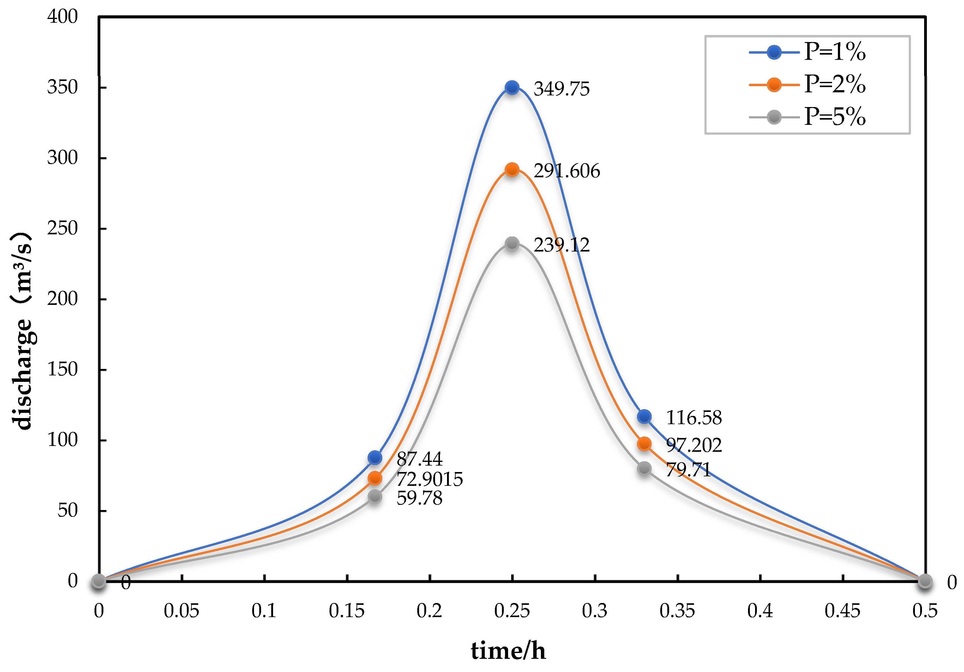
Figure 3.
Hazard zoning diagram of debris flow under different frequencies: (a) p = 1%; (b) p = 2%; (c) p = 5%.
Figure 3.
Hazard zoning diagram of debris flow under different frequencies: (a) p = 1%; (b) p = 2%; (c) p = 5%.

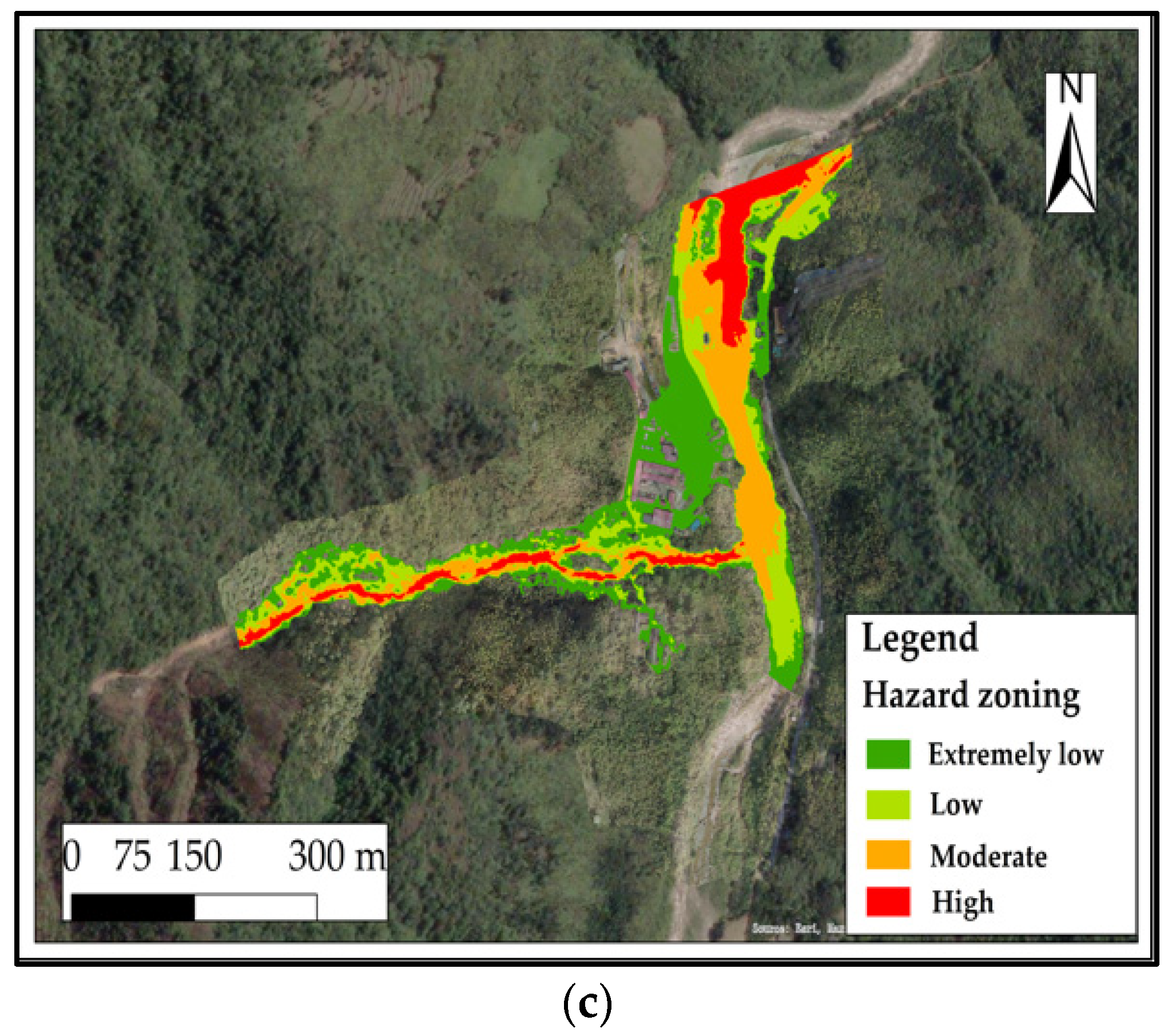
Figure 4.
Interpretation of the LT works in the study area.

Figure 5.
Experiment setups: (a) the flume; (b) sensor; (c) data logger; and (d) debris flow and its arrangement.
Figure 5.
Experiment setups: (a) the flume; (b) sensor; (c) data logger; and (d) debris flow and its arrangement.
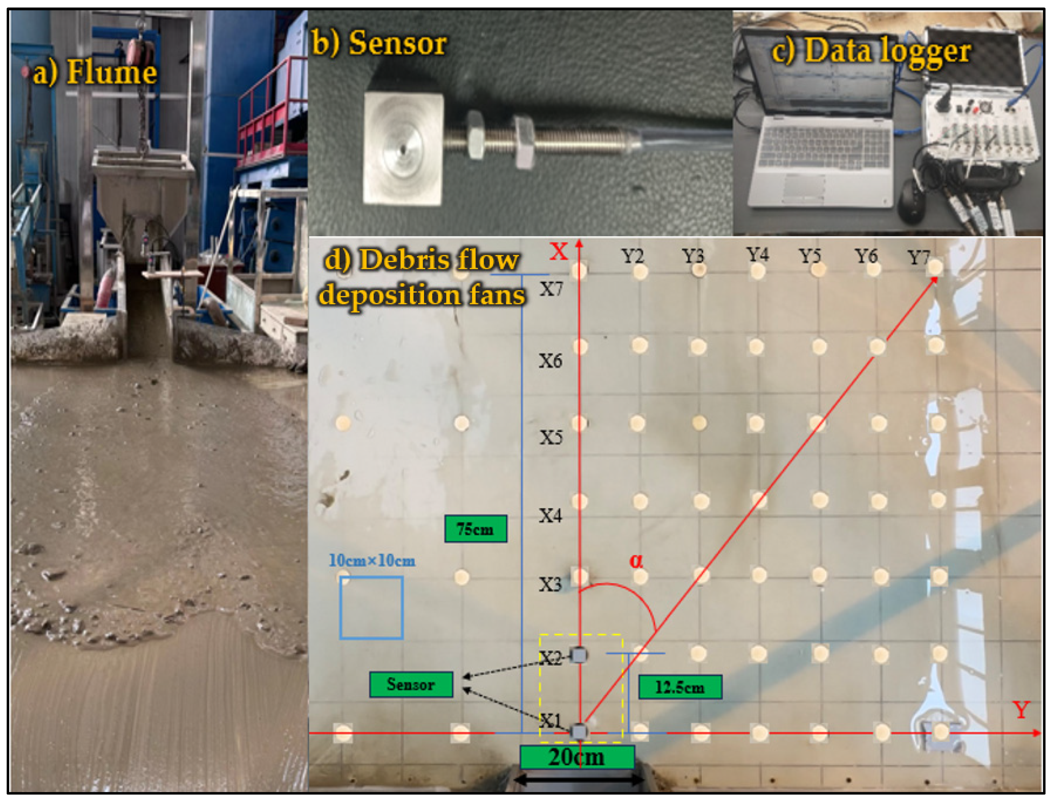
Figure 6.
Arrangement of different flow directions of sensors.
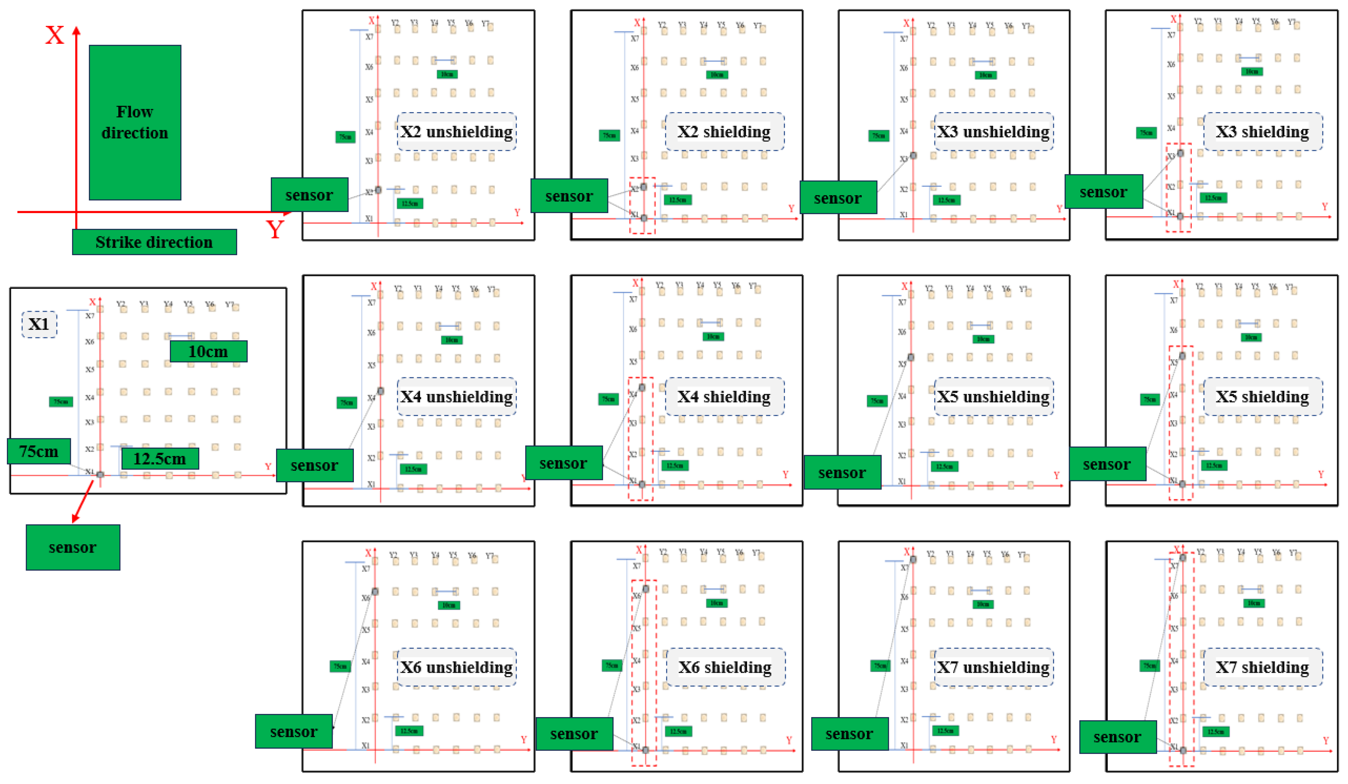
Figure 7.
Arrangement of different strike directions of sensors.
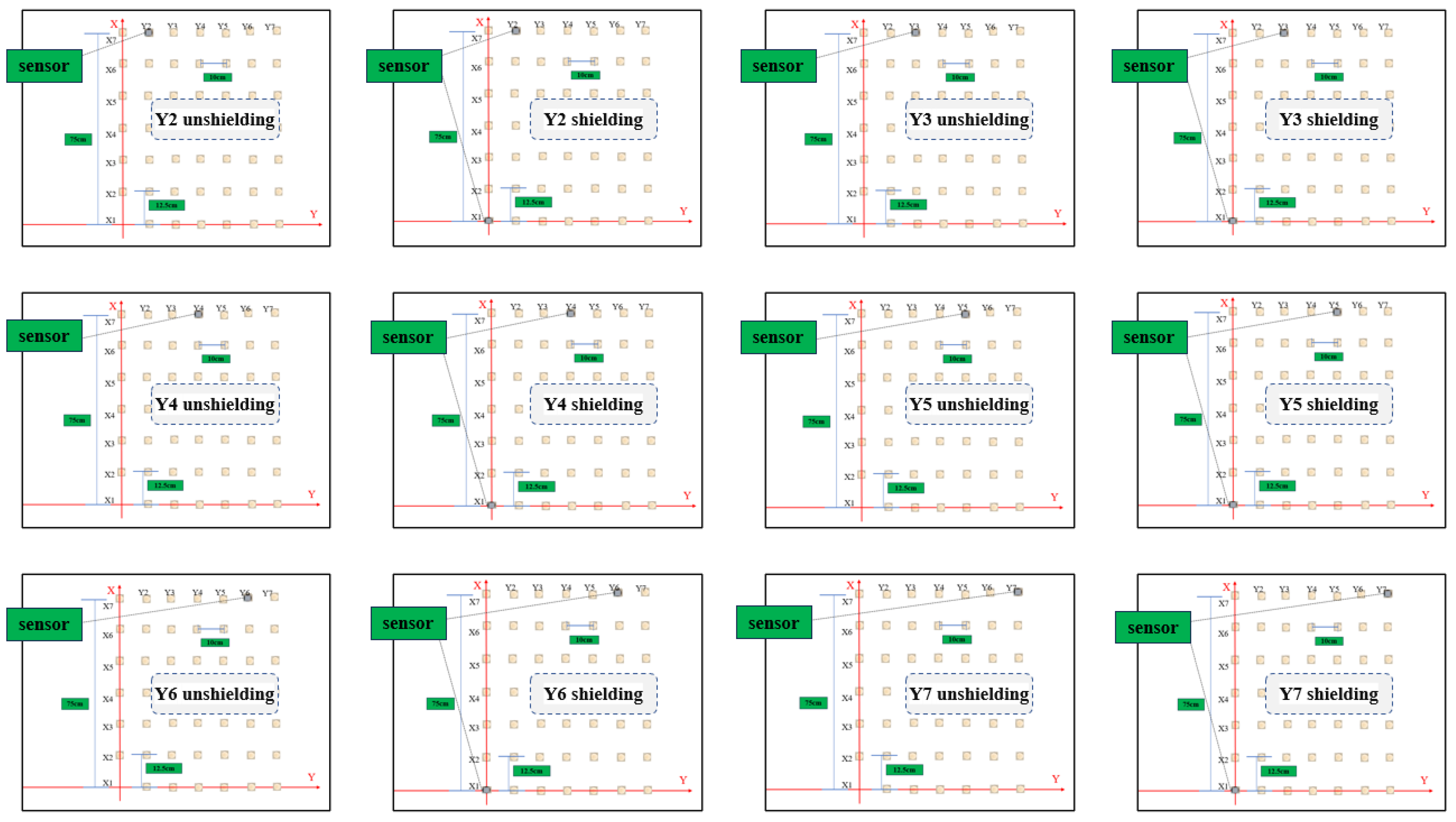
Figure 8.
Impact force variation curve 1: (a) impact force and location of the building; (b) change of impact force at the shielded building.
Figure 8.
Impact force variation curve 1: (a) impact force and location of the building; (b) change of impact force at the shielded building.
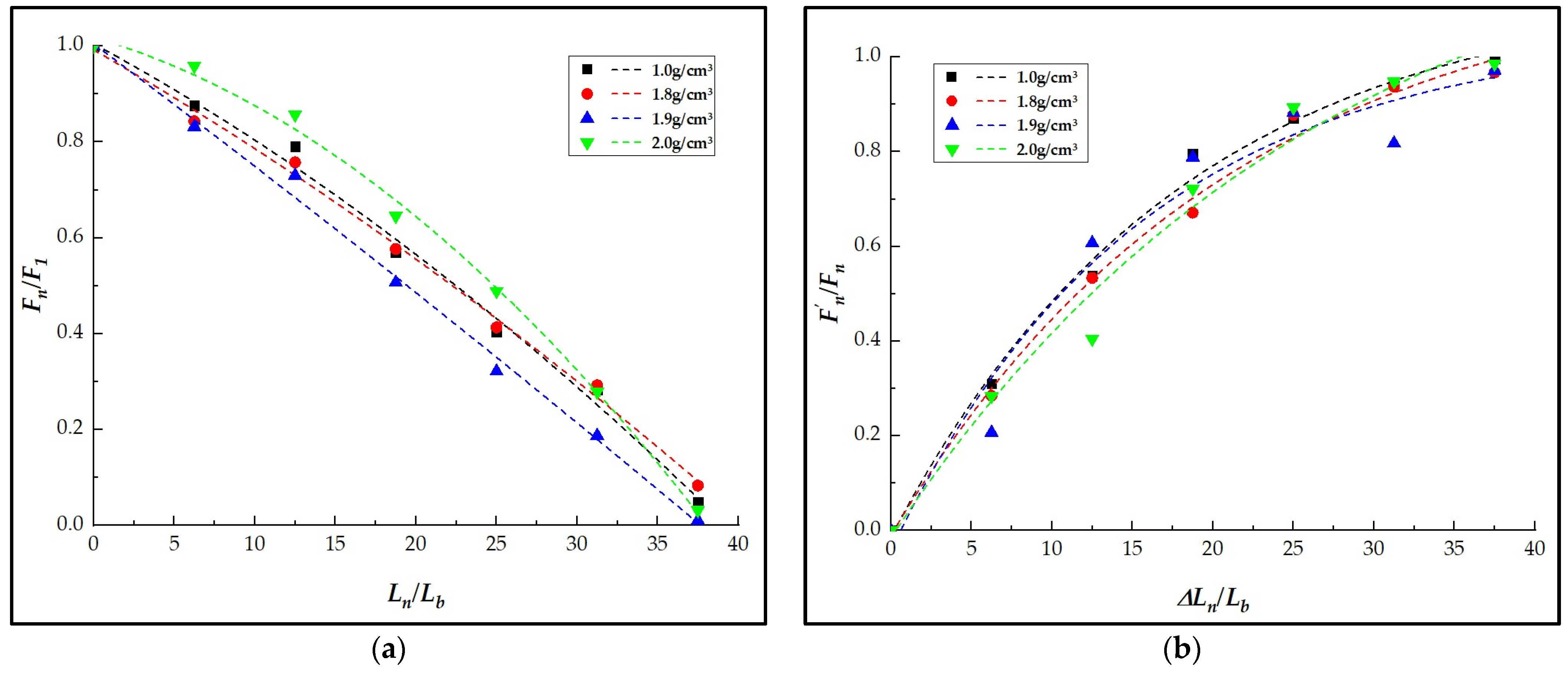
Figure 9.
Impact force variation curve 2: with radians as the horizontal axis.
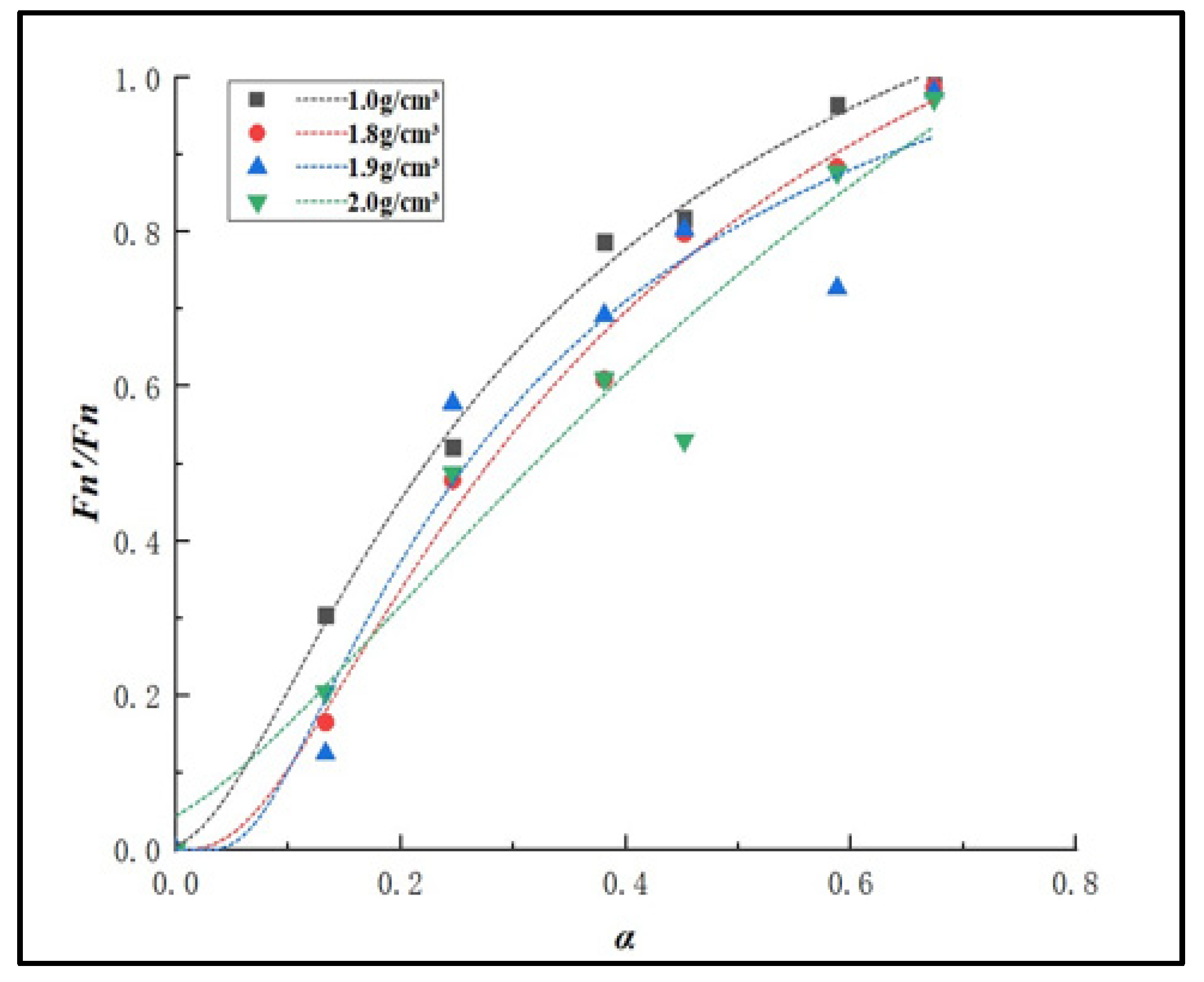
Figure 10.
Detailed construction camp plan.
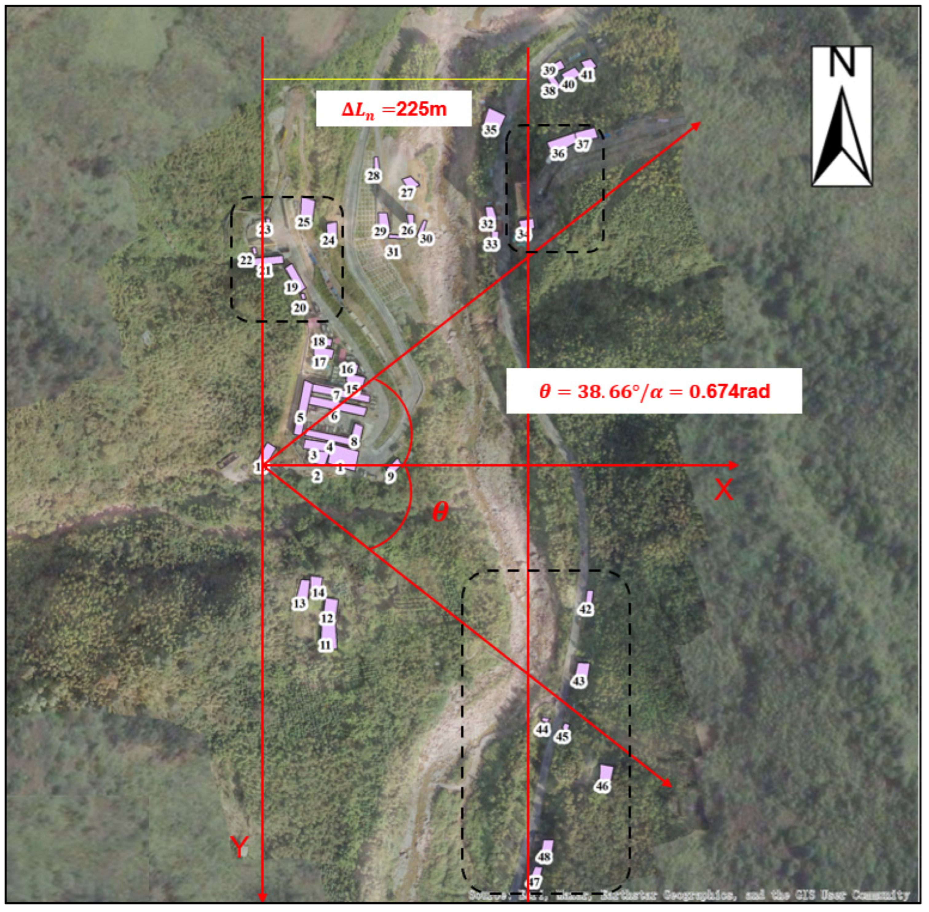
Figure 11.
Vulnerability zoning of tunnel camp: (a) index-based vulnerability zoning map; (b) vulnerability zoning map after experimental correction.
Figure 11.
Vulnerability zoning of tunnel camp: (a) index-based vulnerability zoning map; (b) vulnerability zoning map after experimental correction.

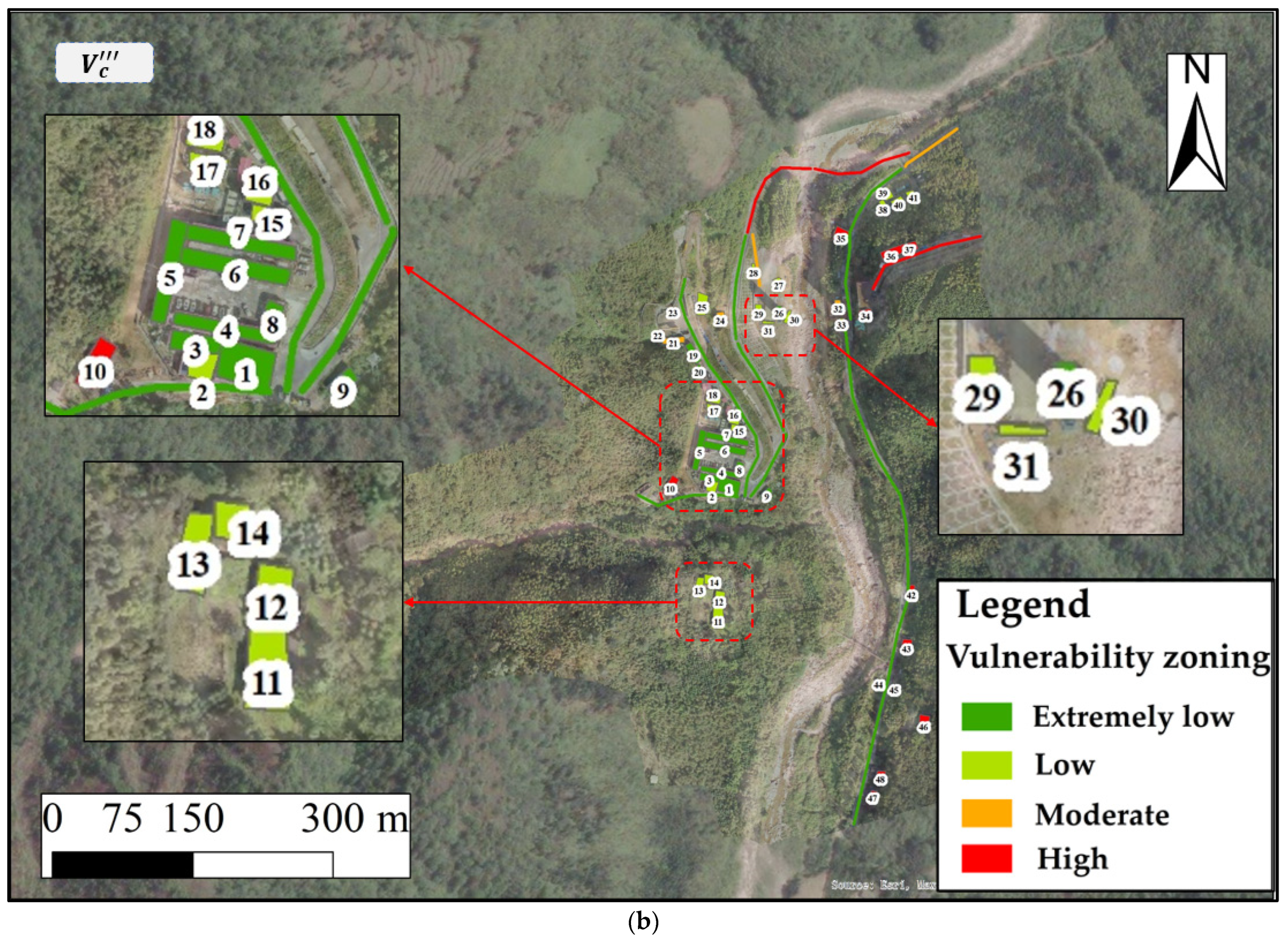
Figure 12.
Risk zoning of LT works in the study area with a probability of 5%.
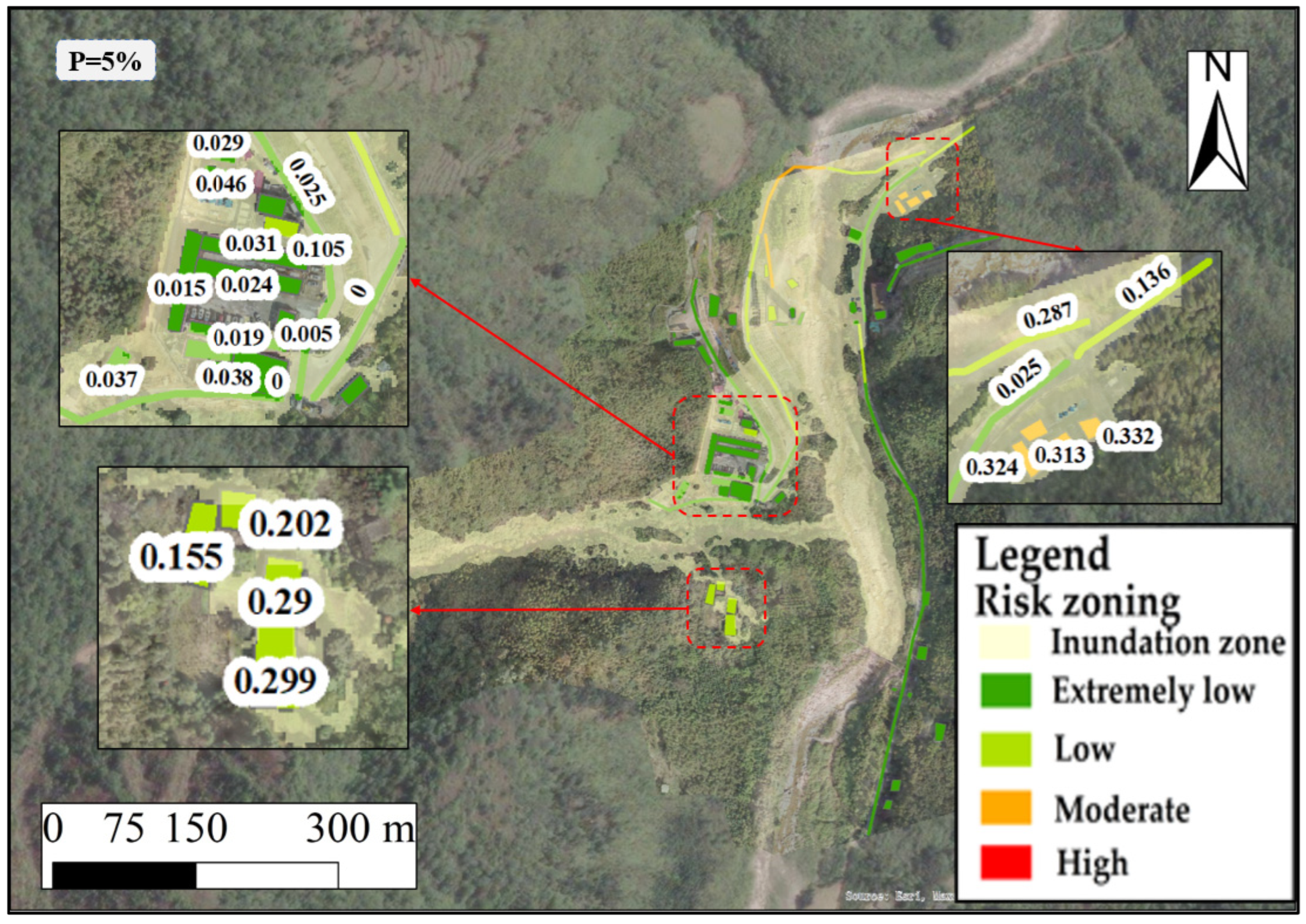
Table 1.
Parameter values for the Jinjia Gully watershed.
| /% | /(kN·m−3) | /h | ||||
|---|---|---|---|---|---|---|
| 1 | 20.0 | 0.954 | 80.527 | 8.053 | 0.826 | 1.538 |
| 2 | 19.0 | 0.949 | 77.654 | 8.343 | 0.776 | 1.200 |
| 5 | 18.0 | 0.941 | 72.147 | 8.926 | 0.757 | 0.941 |
Table 2.
Peak discharge at the section of outlet point under different rainfall frequencies in Jinjia Gully watershed.
Table 2.
Peak discharge at the section of outlet point under different rainfall frequencies in Jinjia Gully watershed.
| /% | /(m3·s−1) | /(m3·s−1) |
|---|---|---|
| 1 | 68.902 | 349.750 |
| 2 | 66.274 | 291.606 |
| 5 | 61.598 | 239.120 |
Table 3.
Main parameters of FLO-2D numerical simulation of Jinjia Gully debris flow.
| Parameter Items | Values | |
|---|---|---|
| Manning’s coefficient () | 0.3 | |
| Volume concentration () | 0.45 | |
| Laminar flow resistance coefficient () | 2280 | |
| Viscous coefficient () | 0.0248 | |
| 14.62 | ||
| Yield stress coefficient () | 0.00236 | |
| 11.24 |
Table 4.
Comparison between the simulation and calculation results of the total amount of solid material washed out in the debris flow under three rainfall frequencies.
Table 4.
Comparison between the simulation and calculation results of the total amount of solid material washed out in the debris flow under three rainfall frequencies.
| /% | Sim. Results/m3 | Calc. Results/m3 | Error/% |
|---|---|---|---|
| 1 | 71,011.72 | 77,077.19 | 8.54 |
| 2 | 51,601.28 | 57,827.64 | 12.07 |
| 5 | 38,770.41 | 42,150.47 | 8.72 |
Table 5.
Assessment factors and values of vulnerability of LT works (buildings).
| Primary Indicators | Weight | Secondary Indicators | Weight | Evaluation Score Y | ||||||
|---|---|---|---|---|---|---|---|---|---|---|
| Engineering Type C1 | 0.2 | Material Storage Shed X1 | 0.05 | 0.4 | ||||||
| Ash Pond X2 | 0.05 | 0.5 | ||||||||
| Explosives Storage X3 | 0.15 | 0.7 | ||||||||
| Power Station X4 | 0.10 | 0.7 | ||||||||
| Air Supply Station X5 | 0.05 | 0.6 | ||||||||
| Water Supply Station X6 | 0.05 | 0.6 | ||||||||
| Concrete Mixing Station X7 | 0.06 | 0.5 | ||||||||
| Aggregate Mixing Station X8 | 0.06 | 0.5 | ||||||||
| Beam Storage Yard X9 | 0.05 | 0.3 | ||||||||
| Track Joint Assembly Yard X10 | 0.05 | 0.3 | ||||||||
| Long Rail Welding Yard X11 | 0.05 | 0.3 | ||||||||
| Steel Beam Assembly Yard X12 | 0.05 | 0.4 | ||||||||
| Ballast Storage Yard X13 | 0.05 | 0.4 | ||||||||
| Other Materials Warehouse X14 | 0.05 | 0.5 | ||||||||
| Residential Area X15 | 0.10 | 0.7 | ||||||||
| Office Area X16 | 0.02 | 0.5 | ||||||||
| Other Living Utility Area X17 | 0.01 | 0.3 | ||||||||
| Structural Characteristics C2 | 0.4 | Structural Type X18 | 0.4 | 0.2 (Steel) | 0.4 (RC) | 0.6 (BC) | 0.7 (Container) | 0.8 (MP House) | ||
| Number of Floors X19 | 0.3 | 0.8 (1–2 Floors) | 0.6 (2–4 Floors) | |||||||
| Construction Time X20 | 0.3 | 0.2 (2 yrs ago) | 0.4 (5 yrs ago) | 0.6 (10 yrs ago) | ||||||
| Construction Quality C3 | 0.4 | Degree of Deformation X21 | 0.6 | 0.1 (None) | 0.4 (Minor) | 0.7 (Significant) | ||||
| Crack Length X22 | 0.2 | 0.1 (<0.5 m) | 0.4 (0.5~1.0 m) | 0.7 (>1.0 m) | ||||||
| Crack Width X23 | 0.2 | 0.1 (<0.1 m) | 0.4 (0.1~0.3 m) | 0.7 (>0.3 m) | ||||||
Table 6.
Assessment factors and values of vulnerability of LT works (access and bridge).
| Primary Indicators | Weight | Secondary Indicators | Weight | Evaluation Score Y | |||||
|---|---|---|---|---|---|---|---|---|---|
| Engineering Type C1 | 0.2 | Construction Access X1 | 0.5 | 0.7 | |||||
| Construction Bridge X2 | 0.5 | 0.7 | |||||||
| Structural Characteristics C2 | 0.4 | Structural Type X3 | 0.6 | 0.7 (other) | 0.6 (concrete) | 0.6 (cement) | 0.7 (asphalt) | ||
| Construction Time X4 | 0.4 | 0.2 (2 yrs ago) | 0.4 (5 yrs ago) | 0.6 (10 yrs ago) | |||||
| Construction Quality C3 | 0.4 | Degree of Deformation X5 | 0.6 | 0.1 (None) | 0.4 (Minor) | 0.7 (Significant) | |||
| Crack Length X6 | 0.2 | 0.1 (<0.5 m) | 0.4 (0.5~1.0 m) | 0.7 (>1.0 m) | |||||
| Crack Width X7 | 0.2 | 0.1 (<0.1 m) | 0.4 (0.1~0.3 m) | 0.7 (>0.3 m) | |||||
Table 7.
Vulnerability value for LT works (Buildings).
| ID | (Floors) | (Yrs Ago) | (m) | (m) | |||||
|---|---|---|---|---|---|---|---|---|---|
| 1 | X12 | Steel | 1 | 5 | Minor | 0.5~1 | 0.1~0.3 | 0.34 | 0.005 |
| 2 | X14 | Container | 2 | 5 | Significant | 0.5~1 | 0.1~0.3 | 0.493 | 0.703 |
| 3 | X14 | Container | 2 | 5 | Minor | 0.5~1 | 0.1~0.3 | 0.421 | 0.374 |
| 4 | X15 | RC | 2 | 5 | Minor | 0.5~1 | 0.1~0.3 | 0.382 | 0.196 |
| 5 | X16 | RC | 2 | 5 | Minor | 0.5~1 | 0.1~0.3 | 0.37 | 0.142 |
| 6 | X15 | RC | 2 | 5 | Minor | 0.5~1 | 0.1~0.3 | 0.382 | 0.196 |
| 7 | X17 | MP House | 2 | 5 | Minor | 0.5~1 | 0.1~0.3 | 0.433 | 0.427 |
| 8 | X16 | RC | 2 | 5 | Minor | 0.5~1 | 0.1~0.3 | 0.37 | 0.142 |
| 9 | X15 | BC | 2 | 10 | Significant | >1 | >0.3 | 0.558 | 1 |
| 10 | X14 | Container | 2 | 5 | Significant | >1 | >0.3 | 0.541 | 0.922 |
| 11 | X15 | BC | 2 | 10 | Significant | >1 | >0.3 | 0.558 | 1 |
| 12 | X15 | BC | 2 | 10 | Significant | >1 | >0.3 | 0.558 | 1 |
| 13 | X15 | BC | 2 | 10 | Significant | >1 | >0.3 | 0.558 | 1 |
| 14 | X15 | BC | 2 | 10 | Significant | >1 | >0.3 | 0.558 | 1 |
| 15 | X6 | MP House | 1 | 5 | Minor | 0.5~1 | 0.1~0.3 | 0.438 | 0.452 |
| 16 | X9 | RC | 2 | 5 | Significant | >1 | >0.3 | 0.491 | 0.694 |
| 17 | X8 | BC | 1 | 5 | Significant | >1 | >0.3 | 0.526 | 0.854 |
| 18 | X7 | BC | 1 | 5 | Significant | >1 | >0.3 | 0.526 | 0.854 |
| 19 | X10 | Steel | 1 | 5 | Minor | 0.5~1 | 0.1~0.3 | 0.339 | 0 |
| 20 | X4 | RC | 1 | 5 | Minor | 0.5~1 | 0.1~0.3 | 0.382 | 0.196 |
| 21 | X12 | Steel | 1 | 5 | Significant | >1 | >0.3 | 0.46 | 0.553 |
| 22 | X15 | BC | 2 | 10 | Significant | >1 | >0.3 | 0.558 | 1 |
| 23 | X15 | BC | 2 | 10 | Significant | >1 | >0.3 | 0.558 | 1 |
| 24 | X10 | Steel | 1 | 5 | Significant | >1 | >0.3 | 0.459 | 0.548 |
| 25 | X11 | Steel | 1 | 5 | Significant | 0.5~1 | >0.3 | 0.435 | 0.438 |
| 26 | X13 | RC | 1 | 5 | Minor | 0.5~1 | 0.1~0.3 | 0.372 | 0.151 |
| 27 | X14 | BC | 2 | 5 | Minor | 0.5~1 | 0.1~0.3 | 0.405 | 0.301 |
| 28 | X6 | MP House | 1 | 5 | Minor | 0.5~1 | 0.1~0.3 | 0.438 | 0.452 |
| 29 | X12 | Steel | 1 | 5 | Significant | >1 | >0.3 | 0.46 | 0.553 |
| 30 | X11 | Steel | 1 | 5 | Significant | >1 | >0.3 | 0.459 | 0.548 |
| 31 | X7 | RC | 1 | 5 | Significant | >1 | >0.3 | 0.494 | 0.708 |
| 32 | X5 | BC | 1 | 5 | Significant | 0.5~1 | >0.3 | 0.502 | 0.744 |
| 33 | X4 | BC | 2 | 5 | Minor | 0.5~1 | 0.1~0.3 | 0.414 | 0.342 |
| 34 | X15 | BC | 2 | 10 | Significant | >1 | >0.3 | 0.558 | 1 |
| 35 | X15 | BC | 2 | 10 | Significant | >1 | >0.3 | 0.558 | 1 |
| 36 | X15 | BC | 2 | 10 | Significant | >1 | >0.3 | 0.558 | 1 |
| 37 | X15 | BC | 2 | 10 | Significant | >1 | >0.3 | 0.558 | 1 |
| 38 | X14 | BC | 2 | 10 | Minor | 0.5~1 | 0.1~0.3 | 0.429 | 0.411 |
| 39 | X14 | BC | 2 | 10 | Minor | 0.5~1 | 0.1~0.3 | 0.429 | 0.411 |
| 40 | X14 | BC | 2 | 10 | Minor | 0.5~1 | 0.1~0.3 | 0.429 | 0.411 |
| 41 | X14 | BC | 2 | 10 | Minor | 0.5~1 | 0.1~0.3 | 0.429 | 0.411 |
| 42 | X15 | BC | 2 | 10 | Significant | >1 | >0.3 | 0.558 | 1 |
| 43 | X15 | BC | 2 | 10 | Significant | >1 | >0.3 | 0.558 | 1 |
| 44 | X15 | BC | 1 | 10 | Significant | >1 | >0.3 | 0.558 | 1 |
| 45 | X15 | BC | 2 | 10 | Minor | 0.5~1 | 0.1~0.3 | 0.438 | 0.452 |
| 46 | X15 | BC | 2 | 10 | Significant | >1 | >0.3 | 0.558 | 1 |
| 47 | X15 | BC | 2 | 10 | Significant | >1 | >0.3 | 0.558 | 1 |
| 48 | X15 | BC | 1 | 10 | Significant | >1 | >0.3 | 0.558 | 1 |
Table 8.
Vulnerability value for LT works (access and bridge).
| ID | (Yrs Ago) | (m) | (m) | |||||
|---|---|---|---|---|---|---|---|---|
| 1 | X1 | Cement | 5 | Minor | 0.5~1 | 0.1~0.3 | 0.438 | 0.188 |
| 2 | X1 | Cement | 5 | Minor | 0.5~1 | 0.1~0.3 | 0.438 | 0.188 |
| 3 | X1 | Cement | 5 | Minor | 0.5~1 | 0.1~0.3 | 0.438 | 0.188 |
| 4 | X1 | Cement | 5 | Minor | 0.5~1 | 0.1~0.3 | 0.438 | 0.188 |
| 5 | X1 | Cement | 5 | Minor | 0.5~1 | 0.1~0.3 | 0.438 | 0.188 |
| 6 | X1 | Asphalt | 5 | Significant | 0.5~1 | 0.1~0.3 | 0.534 | 0.938 |
| 7 | X1 | Asphalt | 10 | Significant | 0.5~1 | <0.1 | 0.542 | 1 |
| 8 | X1 | Other | 10 | Minor | 0.5~1 | 0.1~0.3 | 0.494 | 0.625 |
| 9 | X1 | Asphalt | 5 | Minor | 0.5~1 | <0.1 | 0.438 | 0.188 |
| 10 | X1 | Asphalt | 5 | Minor | 0.5~1 | <0.1 | 0.438 | 0.188 |
| 11 | X1 | Concrete | 5 | Significant | 0.5~1 | <0.1 | 0.486 | 0.563 |
| 12 | X1 | Other | 10 | Significant | 0.5~1 | <0.1 | 0.542 | 1 |
| 13 | X1 | Cement | 5 | Minor | 0.5~1 | <0.1 | 0.414 | 0 |
| 14 | X1 | Asphalt | 5 | Minor | 0.5~1 | <0.1 | 0.438 | 0.188 |
Table 9.
Classification of the vulnerability of LT works.
| 0.8~1.0 | 0.5~0.8 | 0.2~0.5 | 0~0.2 | |
|---|---|---|---|---|
| Level | High | Moderate | Low | Extremely low |
Table 10.
Formula coefficient 1.
| a | b | c | R2 | |
|---|---|---|---|---|
| 1.0 | −1.9 × 10⁻⁴ ± 9.3 × 10⁻⁵ | −0.018 ± 0.004 | 1.005 ± 0.029 | 0.9906 |
| 1.8 | −1.2 × 10⁻⁴ ± 6.9 × 10⁻⁵ | −0.019 ± 0.003 | 0.992 ± 0.021 | 0.9942 |
| 1.9 | −3.9 × 10⁻⁵ ± 8.2 × 10⁻⁵ | −0.025 ± 0.003 | 1.005 ± 0.026 | 0.9934 |
| 2.0 | −4.5 × 10⁻⁴ ± 7.4 × 10⁻⁵ | −0.009 ± 0.003 | 1.018 ± 0.023 | 0.9947 |
Table 11.
Formula coefficient 2.
| A | B | C | R2 | |
|---|---|---|---|---|
| 1.0 | −1.169 ± 0.068 | 18.041 ± 2.633 | 1.157 ± 0.073 | 0.9914 |
| 1.8 | −1.209 ± 0.087 | 21.133 ± 3.492 | 1.201 ± 0.094 | 0.9913 |
| 1.9 | −1.096 ± 0.143 | 15.506 ± 5.326 | 1.005 ± 0.144 | 0.9431 |
| 2.0 | −1.383 ± 0.263 | 26.691 ± 10.172 | 1.368 ± 0.284 | 0.9694 |
Table 12.
Formula coefficient 3.
| D | F | H | R2 | |
|---|---|---|---|---|
| 1.0 | 1.555 ± 0.121 | −0.316 ± 0.062 | 0.056 ± 0.033 | 0.9957 |
| 1.8 | 1.642 ± 0.282 | −0.373 ± 0.135 | 0.035 ± 0.060 | 0.9862 |
| 1.9 | 1.352 ± 0.434 | −0.257 ± 0.216 | 1.3 × 10⁻¹¹ ± 0.112 | 0.9203 |
| 2.0 | 2.349 ± 1.465 | −0.806 ± 0.699 | 0.202 ± 0.224 | 0.9196 |
Table 13.
Vulnerability value calculation 1.
| ID | (m) | (m) | ||||||
|---|---|---|---|---|---|---|---|---|
| 5 | 25.82 | 6 | 0.215 | 0.175 | 0.191 | 0.193 | 0.370 | 0.071 |
| 11 | 55.99 | 6 | 0.424 | 0.405 | 0.393 | 0.407 | 0.558 | 0.227 |
| 12 | 56.41 | 6 | 0.426 | 0.407 | 0.396 | 0.409 | 0.558 | 0.229 |
| 13 | 30.62 | 6 | 0.251 | 0.216 | 0.226 | 0.231 | 0.558 | 0.129 |
| 14 | 44.87 | 6 | 0.352 | 0.328 | 0.323 | 0.335 | 0.558 | 0.187 |
| 15 | 70.16 | 6 | 0.506 | 0.489 | 0.476 | 0.490 | 0.438 | 0.215 |
| 16 | 65.41 | 6 | 0.479 | 0.462 | 0.449 | 0.463 | 0.491 | 0.228 |
| 17 | 40.75 | 6 | 0.324 | 0.298 | 0.296 | 0.306 | 0.526 | 0.161 |
| 18 | 38.26 | 6 | 0.307 | 0.279 | 0.279 | 0.288 | 0.526 | 0.152 |
| 26 | 120.02 | 6 | 0.732 | 0.703 | 0.714 | 0.716 | 0.372 | 0.267 |
| 27 | 121.51 | 6 | 0.737 | 0.708 | 0.720 | 0.722 | 0.405 | 0.292 |
| 28 | 96.67 | 6 | 0.637 | 0.617 | 0.612 | 0.622 | 0.438 | 0.272 |
| 29 | 98.85 | 6 | 0.647 | 0.626 | 0.622 | 0.632 | 0.460 | 0.291 |
| 30 | 125.83 | 6 | 0.753 | 0.722 | 0.738 | 0.737 | 0.459 | 0.338 |
| 31 | 104.77 | 6 | 0.672 | 0.650 | 0.649 | 0.657 | 0.494 | 0.324 |
| 32 | 181.92 | 6 | 0.913 | 0.850 | 0.924 | 0.896 | 0.502 | 0.450 |
| 33 | 183.04 | 6 | 0.916 | 0.852 | 0.927 | 0.898 | 0.414 | 0.372 |
| 35 | 182.19 | 6 | 0.914 | 0.850 | 0.925 | 0.896 | 0.558 | 0.500 |
Table 14.
Vulnerability value calculation 2.
| ID | (m) | (m) | ||||||
|---|---|---|---|---|---|---|---|---|
| 1 | 62.02 | 6 | 0.460 | 0.442 | 0.429 | 0.444 | 0.340 | 0.151 |
| 2 | 43.61 | 6 | 0.344 | 0.319 | 0.315 | 0.326 | 0.493 | 0.161 |
Table 15.
Vulnerability value calculation 3.
| ID | 3 | 4 | 6 | 7 | 8 | 9 |
| (m) | 41.72 | 50.97 | 51.13 | 51.28 | 71.94 | 105.08 |
| (m) | 6 | 6 | 6 | 6 | 6 | 6 |
| (rad) | 0.204 | 0.296 | 0.573 | 0.631 | 0.263 | 0.172 |
| 0.331 | 0.392 | 0.393 | 0.394 | 0.515 | 0.673 | |
| 0.305 | 0.371 | 0.372 | 0.373 | 0.499 | 0.651 | |
| 0.302 | 0.362 | 0.363 | 0.364 | 0.485 | 0.650 | |
| 0.313 | 0.375 | 0.376 | 0.377 | 0.500 | 0.658 | |
| 0.345 | 0.532 | 0.889 | 0.938 | 0.470 | 0.271 | |
| 0.384 | 0.567 | 0.863 | 0.900 | 0.509 | 0.303 | |
| 0.323 | 0.466 | 0.830 | 0.893 | 0.415 | 0.272 | |
| 0.350 | 0.522 | 0.861 | 0.910 | 0.465 | 0.282 | |
| 0.110 | 0.196 | 0.324 | 0.343 | 0.232 | 0.186 | |
| 0.421 | 0.382 | 0.382 | 0.433 | 0.370 | 0.558 | |
| 0.046 | 0.075 | 0.124 | 0.149 | 0.086 | 0.104 |
Table 16.
Classification of risk levels and their characteristic descriptions for large-scale temporary works.
Table 16.
Classification of risk levels and their characteristic descriptions for large-scale temporary works.
| Risk Levels | Characteristic Descriptions |
|---|---|
| Extremely low | The hazard of debris flows and the vulnerability of the LT works are both low. There is minimal risk of damage to the LT works from debris flow hazards, which does not affect normal operations. |
| Low | The damage caused by debris flows is minor, with a low vulnerability of the LT works. The overall risk value of debris flow disasters is low, and they have minimal impact on normal operations. |
| Moderate | The hazard level of debris flow disasters is moderate, affecting the normal operation of the LT works. It is necessary to design and construct debris flow disaster prevention and control projects of different levels to ensure the normal operation of transportation. |
| High | The hazard of debris flows and the vulnerability of the LT works are both high, with debris flows causing significant damage to engineering structures and severely impacting their operation. Alongside strengthening debris flow prevention and control measures, it is necessary to enhance monitoring and early warning measures. In severe cases, measures such as rerouting or selecting new routes should be taken based on the specific conditions of the road sections. |
Disclaimer/Publisher’s Note: The statements, opinions and data contained in all publications are solely those of the individual author(s) and contributor(s) and not of MDPI and/or the editor(s). MDPI and/or the editor(s) disclaim responsibility for any injury to people or property resulting from any ideas, methods, instructions or products referred to in the content. |
© 2024 by the authors. Licensee MDPI, Basel, Switzerland. This article is an open access article distributed under the terms and conditions of the Creative Commons Attribution (CC BY) license (https://creativecommons.org/licenses/by/4.0/).
Share and Cite
MDPI and ACS Style
Wu, Y.; Lei, Y.; Gu, H. Debris Flow Risk Assessment for the Large-Scale Temporary Work Site of Railways—A Case Study of Jinjia Gully, Tianquan County. Water 2024, 16, 1152. https://doi.org/10.3390/w16081152
AMA Style
Wu Y, Lei Y, Gu H. Debris Flow Risk Assessment for the Large-Scale Temporary Work Site of Railways—A Case Study of Jinjia Gully, Tianquan County. Water. 2024; 16(8):1152. https://doi.org/10.3390/w16081152
Chicago/Turabian StyleWu, Yunpu, Yu Lei, and Haihua Gu. 2024. "Debris Flow Risk Assessment for the Large-Scale Temporary Work Site of Railways—A Case Study of Jinjia Gully, Tianquan County" Water 16, no. 8: 1152. https://doi.org/10.3390/w16081152
Note that from the first issue of 2016, this journal uses article numbers instead of page numbers. See further details here.