Application of One-Dimensional Hydrodynamic Coupling Model in Complex River Channels: Taking the Yongding River as an Example

Abstract

River conditions are complex and affected by human activities. Various hydraulic structures change the longitudinal slope and cross-sectional shape of the riverbed, which has a significant impact on the simulation of water-head evolution. With continuous population growth, the hydrological characteristics of the Yongding River Basin have undergone significant changes. Too little or too much water discharge may be insufficient to meet downstream ecological needs or lead to the wastage of water resources, respectively. It is necessary to consider whether the total flow in each key section can achieve the expected value under different discharge flows. Therefore, a reliable computer model is needed to simulate the evolution of the water head and changes in the water level and flow under different flow rates to achieve efficient water resource allocation. A one-dimensional hydrodynamic coupling model based on the Saint-Venant equations was established for the Yongding River Basin. Different coupling methods were employed to calibrate the coupling model parameters, using centralised water replenishment data for the autumn of 2022, and the simulation results were verified using centralised water replenishment data for the spring of 2023. The maximum error of the water-head arrival time between different river sections was 4 h, and the maximum error of the water-head arrival time from the Guanting Reservoir to each key cross-section was 6 h. The maximum flow error was less than 5 m³/s, and the changing trend of the flow over time was consistent with the measured data. The model effectively solved the problem of low accuracy of the water level and flow calculation results when using the traditional one-dimensional hydrodynamic model to simulate the flow movement of complex river channels in the Yongding River. The output results of the model include the time when the water head arrives at the key section, the change process of the water level and flow of each section, the change process of the water storage of lakes and gravel pits, and the change process of the total flow and water surface area of the key section. This paper reports data that support the development of an ecological water compensation scheme for the Yongding River.

1. Introduction

The numerical simulation of river hydrodynamics is of great significance for the scientific planning and water allocation of cities around rivers. The study of fluid mechanics mainly focuses on the power wave equation (i.e., the complete set of Saint-Venant equations). At present, various river and coastal hydrodynamic models based on the Saint-Venant equation, such as ISIS, MIKE 11, HEC-RAS, TUFLOW, and other general hydrodynamic models, are widely used for large-scale river flow and flood prediction [1,2,3,4]. However, it is difficult for these models to carry out secondary development. For rivers with complex underlying surface conditions, developing a general model according to the actual state of the river is challenging, as is integration into the self-developed model platform. Moreover, because of the complexity of natural rivers, it is difficult to guarantee the calculation accuracy of a general model when simulating rivers with many lake pits, variable river infiltration, and variable roughness of the main channel [5]. Therefore, according to actual river characteristics, a self-developed model was used to simulate complex river flow movements and thus improve simulation accuracy. Most self-developed models use the finite difference method to solve the Saint-Venant equations, simulating the evolution of a river head, such as that developed by Wang [6]. He proposed the use of various finite difference schemes (such as the leapfrog, Lax-Wendroff, Abbott implicit, and Pressimann implicit schemes) to solve one-dimensional unsteady problems. In this study, the Pressimann implicit scheme is used to solve the Saint-Venant equations. This approach has the advantages of high calculation accuracy, a stable calculation process, and strong adaptability, which are beneficial for improving the stability of the model when calculating complex terrain [7,8].

The river below the Guanting Reservoir in the Yongding River Basin is divided into mountain gorges and plain sections. There is a large height drop in the mountain gorge section, and two reservoirs, Luopoling and Zhuwo, have been constructed [9,10]. The drop in terrain height at the outlet of the reservoir was greater than 10 m. Owing to the influence of sand mining for many years, the plain section of the river channel has undergone great terrain changes and is affected by changes in hydrological conditions. The river channel has dried up year-round, and a large amount of vegetation has grown. These factors complicate the river channel of the Yongding River, and problems emerge, such as significant changes in the shape of the river section, changes in the elevation of the river bottom, increased roughness of the main river channel, as well as blockage of rivers, lakes, and depressions by reservoirs and control projects [11,12,13]. When using the traditional one-dimensional hydrodynamic model, these problems can lessen the accuracy of the model simulation and even stop the model from running [14].

Therefore, this study examines the centralised ecological water compensation data of the Yongding River across different periods and analyses the control engineering, river section changes, roughness changes among different rivers, as well as river infiltration in the Yongding River channel on a spatial scale. The river channel was divided according to the actual state of the river. Subsequently, a hydrodynamic coupling model based on the Saint-Venant equations, coupled with a water level and storage calculation model, control engineering, and a lake pit water balance model, was constructed. The coupled model fully considered the roughness and water infiltration of different sections to improve the accuracy of simulated flow time and water volume. Simulation accuracy was verified using the ecologically centralised water replenishment data of the Yongding River. The flow time of the water head in the complex river channel of the Yongding River and the water level and flow changes in the key sections during the ecologically centralised water replenishment period were simulated. The accuracy was compared with the simulation results of the traditional one-dimensional hydrodynamic model to verify the improvement effect of the constructed coupling model on the simulation accuracy and provide a scientific reference for the centralised ecological water replenishment of the Yongding River.

2. Materials and Methods

2.1. Study Area

The Yongding River Basin originates from Inner Mongolia and Shanxi and flows through Beijing, Hebei, and Tianjin. It is an important tributary of the Haihe River Basin. It is also an important water conservation area, ecological corridor, and ecological barrier in Beijing, Tianjin, and Hebei provinces [15], with a total basin area of 47,856 km². The basin has a seasonal temperate semi-arid climate. The region experiences a multi-year average annual precipitation spanning 550 to 660 million m², 85% of which occurs from June to September. As the largest river in Beijing, the Yongding River has been greatly affected by human activities, the construction of flood control facilities, and water withdrawal over centuries [16]. Due to both to these factors and climate change, the Yongding River has stopped flowing since 1996, resulting in the degradation of its ecological functions. The mountainous and plains sections of the Yongding River lie above and below Sanjiadian, respectively. The reduction of stream flow in the mountainous section led to the loss of freshwater ecosystems of the Yongding River and the formation of bare sandy channels [17]. The river in the plain section was heavily excavated to become a gravel mine and dumping ground for sewage and garbage [18]. The construction of an ecological corridor for the Yongding River began in 2009, and environmental damage was resolved through the construction of five lakes (Mencheng Lake, Lianshi Lake, Yuanbo Lake, Xiaoyue Lake, and Wanping Lake), as well as functional wetlands to gradually restore the ecosystem of the Yongding River Basin. This paper focuses on the section from below the dam of the Guanting Reservoir to Qujiadian as the study area, spanning about 254 km. This stretch of the river is affected by the above factors, contributing to its extremely complicated situation. The mountainous section is high and steep, and river meandering is simultaneously controlled by several reservoirs at the same time. The plain section is mostly a sandy riverbed, the river is always dry, and the infiltration volume is large; plain lakes and numerous gravel pits and barrages are present. The actual state of the watershed is shown in Figure 1.

2.2. Basic Data

Three types of data were used in this study: topographic, remote sensing, and site monitoring.

The topographic data included river cross-sections and digital elevation model (DEM) elevation data. The spacing between channel cross-sectional data points was 500 m. As the quality of the channel cross-sectional data significantly influences the accuracy of the hydrodynamic model simulation results, improving the quality of the channel cross-section can significantly improve the accuracy of the model simulation. Therefore, combining DEM elevation data, fusing the two sets of data, correcting and interpolating the original river cross-sectional data, conducting field research, and modifying the problematic cross-sectional data can improve the quality of cross-sectional data. The initial conditions of the lakes and gravel pits directly affect the simulation accuracy of one-dimensional hydrodynamic models. Remotely sensed image data were used to extract the initial water level of lakes and gravel pits. In addition, the hysteresis effect of lakes and gravel pits on the water head was considered in the model calculations by combining them with the water level reservoir area curves to improve simulation accuracy. Remote sensing image data were used before the simulated centralised water compensation period to extract the initial water surface area. The station monitoring data used the 2022 and 2023 state-centralised water compensation data. The monitoring data of each key cross-section station in the studied river section were selected as the basic data, and the daily water level and flow data recorded at eight monitoring stations after the start of centralised water compensation were used to calibrate the model parameters and analyse the simulation accuracy. Specific data are presented in

Table 1. Basic data.

Name	Data Precision	Corresponding Model	Data Purpose
River cross-sectional data	Interval 500 m	Hydrodynamic model	Basic data
Digital elevation model	2 m	Hydrodynamic model and water balance model	Improving the accuracy of river cross-sectional data
Measured data	Daily flow rate at 8:00 a.m., daily average flow rate (m3/s)	Hydrodynamic model	Basic data
Remote sensing images	2 m (before and after ecological replenishment)	Water balance model	Inverting the initial conditions of lakes and gravel pits
Storage capacity curve	Water level and storage curve	Water balance model	Improving the simulation accuracy of coupled models

.

All river channel data, the water level and flow measurement data and the research area image used in this article are sourced from and authorized by the Haihe Water Resources Commission.

The programming software used in this article is Vision Studio 2012 (Microsoft Corporation, Redmond, WA, USA), and the programming language is Fortran 90.

2.3. Methods

2.3.1. One-Dimensional Hydrodynamic Modelling of Natural River Channels

The process of water flow evolution is a three-dimensional, non-constant, spatiotemporal flow problem. Because this three-dimensional problem involves many influencing factors, many problems arise in numerical solutions, which generally simplify the problem into one- or two-dimensional non-constant flow problems. In practice, the study of river water movement primarily involves calculating each cross-section of the water level, flow, and flow-rate changes over time, while considering the problem of computational efficiency. Therefore, the use of the more efficient one-dimensional non-constant flow problem, along with the general use of the Saint-Vernant system to describe the incompressible continuity of the equations and dynamics in the form of momentum equations is defined as follows:

$${\{}_{\frac{\partial Q}{\partial t}+\frac{\partial }{\partial x}\left(\frac{\alpha Q^2}{A}\right)+gA\frac{\partial Z}{\partial x}+gA{S}_f=0}^{B\frac{\partial Z}{\partial t}+\frac{\partial Q}{\partial x}=0}$$

(1)

The proposed Saint-Venant system of equations consists of a set of first-order hyperbolic-type linear partial differential equations. Currently, Preissman’s four-point implicit format, which has the advantages of a simple structure, fast convergence, unconditional stabilisation, and freedom from time step restrictions, is commonly used to differentially solve this system of equations.

Based on this difference format, the dependent variables and forms of the derivative functions in space and time are as follows:

$$\left.f\left(x,t\right)\right|{}_M=\frac{\theta }{2}\left(f_{j+1}^{n+1}+f_j^{n+1}\right)+\frac{1-\theta }{2}\left(f_{j+1}^n+f_j^n\right)$$

(2)

$$\left.\frac{\partial f}{\partial x}\right|{}_M=\theta \frac{f_{j+1}^{n+1}-f_j^{n+1}}{\Delta x}+\left(1-\theta \right)\frac{f_{j+1}^n-f_j^n}{\Delta x}$$

(3)

$$\left.\frac{\partial f}{\partial t}\right|{}_M=\frac{f_{j+1}^{n+1}+f_j^{n+1}-f_{j+1}^n-f_j^n}{2\Delta t}$$

(4)

where f denotes the derivation function; subscripts j and j + 1 denote the j th and j + 1 th cross-section, and superscripts n and n + 1 represent two adjacent time steps. θ is a spatial weighting coefficient with a value range of 0 ≤ θ < 1.0. To ensure the computational stability of the model, after parameter calibration, θ takes a value of 0.6. Δt is the time step in seconds, and Δx is the spatial step in metres.

Discretising the system of Saint-Venant equations in the Preissman difference format and neglecting the second-order terms yields the following system of linear equations:

$$-Q_j^{n+1}+C_j{Z}_j^{n+1}+Q_{j+1}^{n+1}+C_j{Z}_{j+1}^{n+1}=D_j$$

(5)

$$E_j{Q}_j^{n+1}-F_j{Z}_j^{n+1}+G_j{Q}_{j+1}^{n+1}+F_j{Z}_{j+1}^{n+1}={\Phi }_j$$

(6)

where Q_jⁿ⁺¹ and Z_jⁿ⁺¹ denote the flow rate and water level at n + 1; R represents the hydraulic radius; u represents the flow velocity; and the coefficients C, D, E, F, G are calculated from the hydraulic parameters at the nth moment. The expression is as follows:

$$C_j=\frac{B_{j+\raisebox{1ex}{$1$}\!\left/ \!\raisebox{-1ex}{$2$}\right.}^n}{2\Delta t}$$

(7)

$$D_j=\frac{(1-\theta )}{\theta }(Q_{j+1}^n-Q_j^n)+C_j(Z_{j+1}^n+Z_j^n)$$

(8)

$$E_j=\frac{\Delta x_j}{2\theta \Delta t}-{(\alpha u)}_j^n+{(\frac{g\left|u\right|}{2\theta c^{2}R})}_j^n\Delta x_j$$

(9)

$$G_j=\frac{\Delta x_j}{2\theta \Delta t}+{(\alpha u)}_{j+1}^n+{(\frac{g\left|u\right|}{2\theta c^{2}R})}_{j+1}^n\Delta x_j$$

(10)

$$F_j={(gA)}_{j+\frac{1}{2}}^n$$

(11)

$${\Phi }_j=\frac{\Delta x_j}{2\theta \Delta t}(Q_{j+1}^n+Q_j^n)-\frac{1-\theta }{\theta }[{(\alpha uQ)}_{j+1}^n-{(\alpha uQ)}_j^n]-\frac{1-\theta }{\theta }{(gA)}_{j+\frac{1}{2}}^n(Z_{j+1}^n-Z_j^n)$$

(12)

2.3.2. Modelling Water Level and Storage Curve Calculations

Common storage calculation methods include the cross-section method (using reservoir cross-sectional data for interpolation to calculate reservoir storage), the contour method (using contour segments to calculate the water body volume at different water levels), the triangular grid method (similar to the digital elevation method, in which the coordinate points are positioned at the bottom of the reservoir as the basis for calculating and directly converting the points into a triangular grid surface to obtain storage volume), and the DEM method [19]. However, in practical applications, it has been found that by quantitatively comparing and analysing the accuracy and complexity of the calculation results of each method, calculating the storage volume using DEM elevation data offers the advantages of high accuracy and fast calculation speed compared to other methods using digitised maps with sufficient accuracy [20]. Moreover, this method can be widely used to calculate the storage volume of all types of lakes and larger gravel pits.

Based on the obtained 2 m precision DEM elevation data, the elevation data were converted into grid data. Interconnected elevation points were used to form square and triangular grids. The water surface points at different water levels were connected to the grid points to form a perpendicular line, resulting in N different types of prisms. where A and B are internal square prisms, and C and D are edge triangular prisms (Figure 2). By summing the volume of each prism, the total water volume at a particular water level can be obtained, and the storage capacity at different water levels can be calculated to obtain the lake pit’s water level storage capacity curve.

$$V_A=\frac{S_0\left(h_a+h_b+h_c+h_d\right)}{4}$$

(13)

$$V_B=\frac{S_0\left(4\times h_c\right)}{4}+\frac{S_0((h_a-h_c)+(h_b-h_c)+(h_c-h_c))}{4}$$

(14)

$$V_C=\frac{S_0\left(h_a+h_b+h_c\right)}{3}$$

(15)

$$V_C=\frac{S_0\left(3\times h_a\right)}{3}+\frac{S_0\left((h_b-h_a)+(h_c-h_a)\right)}{3}$$

(16)

$$V_S={\displaystyle \sum _{i=1}^n{V}_{An}}+V_{Bn}+V_{Cn}+V_{Dn}$$

(17)

where S₀ represents the upper surface area of the rhombic column, h_a, h_b, h_c, and h_d represent the distances from the submerged elevation point to the water surface; and V_s represents the total volume of the water body at different water levels. The DEM method for calculating the reservoir capacity of lake pits is more accurate compared to other methods and is suitable for calculating the reservoir capacity curve of any type of lake and pit.

2.3.3. One-Dimensional Hydrodynamic Model with Coupled Control Project Rules

Generally, due to the large height difference in mountain rivers, rapid rainfall convergence, and high river flow velocity, mountain rivers below city plains are significantly affected by flash floods, ensuring that sudden floods during heavy rainfall will not cause flooding disasters on the downstream plains of the city. Usually, large flood storage reservoirs are built in mountainous river channels, and large water gates are built at the ends of mountainous river channels. Therefore, the entire evolution of water flow in mountain rivers is greatly affected by water conservancy projects, and reservoir control and discharge rules must be considered in the hydrodynamic model.

Because the Saint-Venant equation describes the non-constant asymptotic motion of a continuous free-surface body of water, it is important to consider the reservoir discharge control rule in the hydrodynamic model. In mountainous areas, river channels exhibit large height differences and undulations. When the control project plays the role of water obstruction, the flow parameter in the continuous equation is solved with a zero value. This leads to interruptions in the continuity of the water level and flow in the cross-section, thus causing the dispersion of the calculation results for the connected cross-sections in successive time steps.

The location of the reservoir was inserted into the corresponding location in the continuous channel cross-section (Figure 3), and the discharge control rule was considered in the continuous equation of the Saint-Venant system to control flow magnitude in the cross-section below the hydraulic structures by increasing and decreasing collateral flow. The expressions are as follows:

$${\{}_{Q_{ce}=Q_{zw.\mathrm{lpl}}[Q_{zw.\mathrm{lpl}} \left(t\right)>0]}^{Q_{ce}=0.5[Q_{zw.\mathrm{lpl}}\left(t\right)=0]}$$

(18)

$${\{}_{q_2=Q_{j+1}-Q_{ce}}^{q_1=Q_j-Q_{ce}}$$

(19)

$$Q_{j+1}^{t+1}-Q_j^{t+1}+\frac{B^n\ast \Delta x_j}{2\ast \Delta t\ast \theta }(Z_{j+1}^{t+1}+Z_j^{t+1})=\frac{(q_1+q_2)\Delta x_j}{2\theta }-\frac{1-\theta }{\theta }(Q_{j+1}^t-Q_j^t)+\frac{B^n\ast \Delta x_j}{2\ast \Delta t\ast \theta }(Z_{j+1}^t+Z_j^t)$$

(20)

where q₁ and q₂ indicate the side flow of the upper and lower two sections of the reservoir (m³/s); Q_j and Q_j+1 are the flows of the upper and lower reservoirs before and after the gate (m³/s); Q_ce is the control flow, which controls the size of the side flow; Q_zw.lpl is the process of discharging the flow of the ZhuWo and Lo Poling reservoirs.

2.3.4. One-Dimensional Hydrodynamic Modelling of Coupled Water Balance

Because of the complexity of the natural river channel, the flow of water in the river channel should be considered in addition to the influence of channel roughness. The most important influence is the stagnation of water flow evolution caused by impoundments (e.g., lakes, gravel pits) in the river channel. Therefore, the time course of water flow, including pit filling and storage of the lakes and gravel pits, must be considered in the hydrodynamic model.

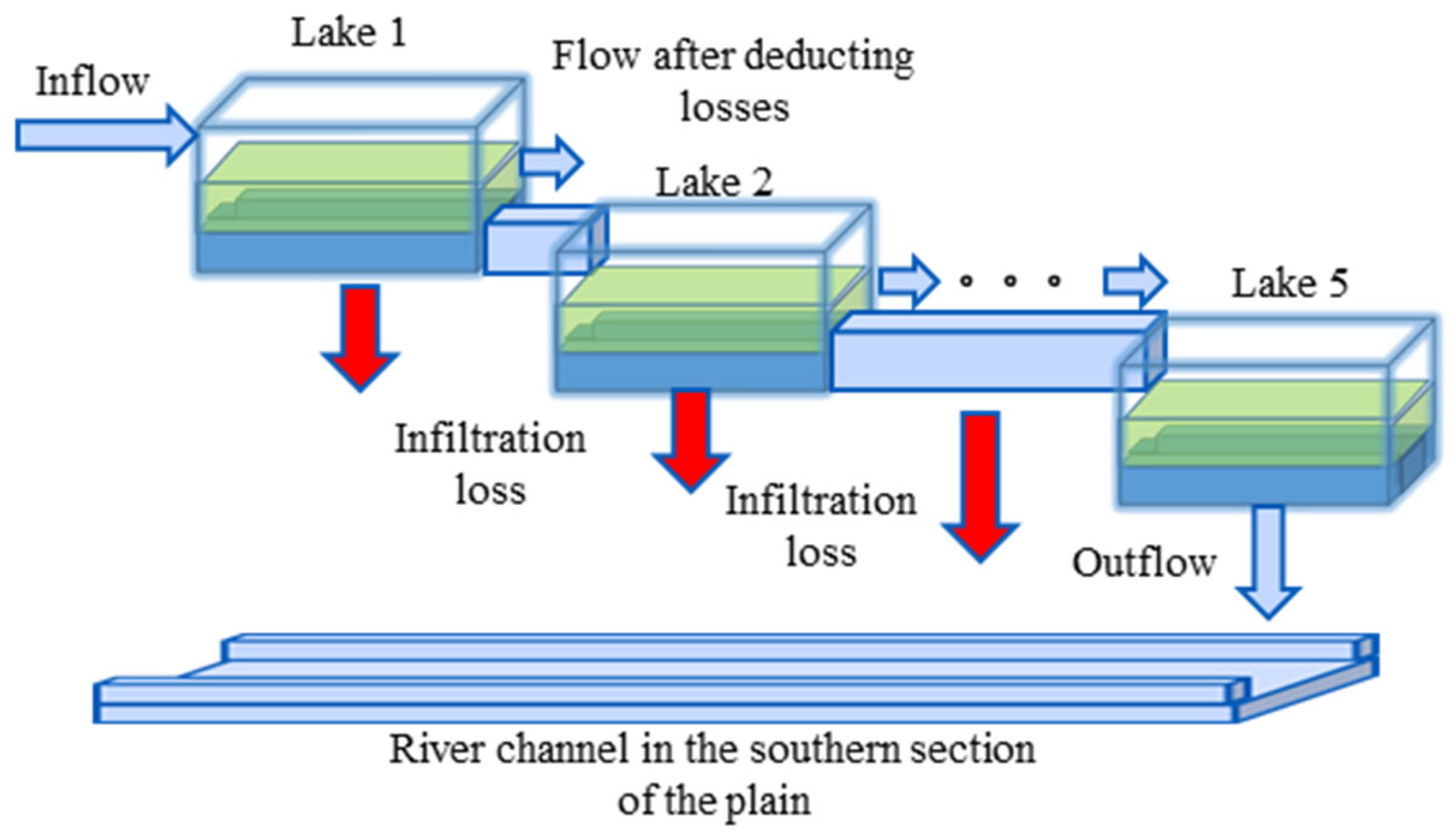
Currently, the one-dimensional hydrodynamic model based on the Saint-Venant equation is unable to simulate the filling and storage process of lake pits. When water flows through the topography of these pits, it loses continuity in the cross-sectional shape and longitudinal slope drop of the channel because the topography and elevation changes are too large. Therefore, the water balance model (Figure 4) and water level storage curve calculated by the reservoir capacity calculation model are coupled into a one-dimensional hydrodynamic model. Coupling methods include loose and tight coupling, which can effectively improve model simulation accuracy.

(1) Loose coupling

Loose coupling, also known as serial coupling, usually refers to two mathematical models for hierarchical coupling; thus, two mathematical models in accordance with a certain order of operation are both interconnected and independent of each other. One or more model interoperability variables is connected to the two mathematical models, so that the model can be run continuously.

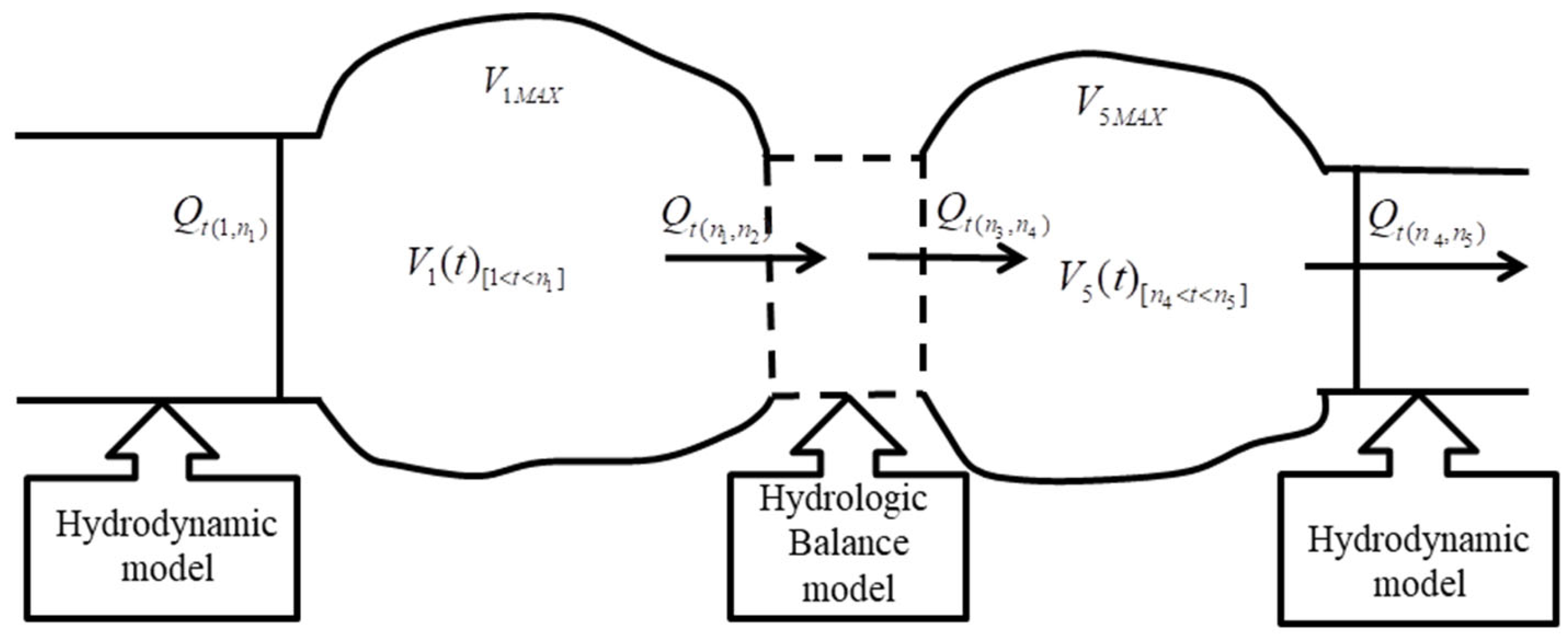
Rivers flowing through plains are typically connected to lakes with larger storage volumes excavated in the river channel, owing to urban planning and urban flood control, which leads to the inability of the traditional one-dimensional hydrodynamic model to calculate such configurations. Therefore, the water balance model can be considered and combined with the water level storage curve to simplify the calculation of this cross-section. Time and flow processes serve as the model coupling variables, the spatial location of the river channel with lakes and gravel pits establishes the hierarchical relationship of the model coupling, and the two mathematical models are serially coupled, as shown in Figure 5.

The numerical expression of the water balance model is shown below.

$$\begin{gathered} \begin{array}{l}{V}_1(t)=V_1(t-1)+Q_t(t=t_0,n_1)\\ t_1=t\\ V_1>V_{1MAX},n_1=t_{v1>V_{1MAX}},Q_{t(1,n_1)}=0\end{array} \\ \begin{array}{l}{V}_2(t)=V_2(t-1)+Q_t(t=n{}_1,n_2)\\ t_2=t\\ V_2>V_{2MAX},n_2=t_{v2>V_{2MAX}},Q_{t(n{}_1,n_2)}=0\end{array} \\ \begin{array}{c}\cdots \end{array} \\ \begin{array}{l}{V}_5(t)=V_5(t-1)+Q_t(t=n{}_4,n_5)\\ t_5=t\\ V_5>V_{5MAX},n_5=t_{v5>V_{5MAX}},Q_{t(n{}_4,n_5)}=0\end{array} \end{gathered}$$

(21)

$$T={\displaystyle \sum _{i=1}^5{t}_i}$$

(22)

In the formula, V₁(t), V₂(t), V₃(t), V₄(t), and V₅(t) indicate the storage volume of five landscape lakes at different moments (cubic metres per second); V_1MAX, V_2MAX, V_3MAX, V_4MAX, and V_5MAX indicate the maximum reservoir capacity of five landscape lakes; Q_t indicates the flow process to reach the coupling point (cubic metres per moment); t indicates the time process, in which t₁, t₂, t₃, t₄, and t₅ indicate the time process of filling and storing, and t₀ indicates the time of the water flow arriving at Sanjiadian; n₁, n₂, n₃, n₄, and n₅ indicate the times at which the five landscape lakes are being filled; and T indicates the total filling and storing time.

(2) Close coupling

Close coupling, also known as parallel coupling, generally refers to the coupling of two mathematical models that can be calculated at the same time step, unlike loose coupling, where the output parameters of one model are directly used as inputs for calculations in another model at the same time step. As the plain sections of the lakes are connected to each other, the flow of water in the continuous lake movement water flow time is negligible; therefore, the lakes can be placed directly into the water balance model for loose coupling calculations. This process involves generalising them into five connected reservoirs, wherein the filling the next reservoir starts once the last reservoir is full. In rivers with long channels and large impoundments in the channel, such as gravel pits scattered at various distances, each gravel pit is also connected through the channel because of the high roughness of the riverbed. This has a significant impact on the evolution of the water flow, and as such, the dynamic evolution time of the water head in the river channel cannot be ignored. Therefore, simplifying and tightly coupling the gravel pit filling and storage processes into a one-dimensional hydrodynamic model (Figure 6) can effectively reduce the problem of error accumulation during model coupling and improve computational efficiency.

The mathematical expression is shown below.

$$B\frac{\partial Z}{\partial t}+\frac{\partial Q}{\partial x}=q_t$$

(23)

$$q_t=-q{(i)}_{lose}-q_p(i)$$

(24)

$${\{}_{q_p(i)=0[V_j(t)>V_j\max ]}^{q_p(i)=Q_i(t)-q{(i)}_{lose}-0.2[V_j(t)<V_j\max ]}$$

(25)

$$V_j(t)=V_j(t-1)+Q_i(t)$$

(26)

$$\frac{\partial Q}{\partial t}+\frac{\partial }{\partial x}\left(\frac{\alpha Q^2}{A}\right)+gA\frac{\partial Z}{\partial x}+gA{S}_f=0$$

(27)

where i denotes the river section number; j denotes the gravel pit serial number; q_t is the side flow; q(i)_lose is the infiltration loss of the river in the spatial step; q_p(i) is the gravel pit diversion flow; Q_i(t) is the flow in this section; V_j(t) is the amount of water in the j th gravel pit; and V_jmax is the maximum storage volume of the j th gravel pit. For the Saint-Venant system of equations, the water balance model was simplified and introduced into the system of equations in the form of lateral flow, considering the location of gravel pits in space and the filling and storage process of gravel pits as a judgment condition to determine the gravel pit diversion flow rate and simulate the time of filling and storage of water flow when passing through the gravel pits. The coupled simplified water balance one-dimensional hydrodynamic model can solve the problem of dispersion of simulation results caused by large changes in slope drop and cross-sectional shape when simulating the location of gravel pits in the traditional one-dimensional hydrodynamic models. In addition, it can simulate the entire process of filling and storage of gravel pits, as well as changes in water level and surface area.

2.3.5. Spatial Coupling of Nodes

Under the influence of the control project, the water movement of the river is more complicated, and if we ignore the discharge flow process of the control project and directly use river data for the simulation, the accuracy of the simulation results will be greatly reduced. Based on the slope drop of the river channel, topographic features, control engineering, and the geographic location of the water point, the entire simulation area was divided into four parts, and the overall elevation gradually decreased from west to east. There were 26 nodes of inflow and outflow, and the nodes were connected to different models in different ways in each section (the nodes include the flow control of the control project, the process of lake pit storage volume change, and the process of flow, inflow, and outflow of the water source point). The locations of each control work and the inflow points were organised, identified on the section space nodes, and coupled into the 1D hydrodynamic model, as shown in Figure 7.

3. Results

In this section, we explain the construction process of the model, as well as the calculation results of the lake pit water level storage curve, the calibration results of river roughness, and river infiltration. The centralised water compensation data of the Yongding River were used to verify the simulation accuracy of the constructed coupled model (the tight and loose coupling of hydrodynamic models with other models), and the simulation results were compared with the simulation results of the uncoupled model (the traditional one-dimensional hydrodynamic model). Thus, the feasibility of coupling models to improve the simulation accuracy was verified.

The Yongding River, below Guanting Hall, passes through mountainous areas, plains, and large lakes, which verifies the accuracy of the model. The model parameters were calibrated using the data measured in autumn 2022, and the model was validated and discussed using the spring data of the centralised water replenishment in the Yongding River in 2023. These data mainly include the flow discharge process of each control project during the water compensation period, the flow process at the diversion and catchment points, the flow and water level monitoring data at key cross-sections, and the manual tracking of water-head monitoring data. The cross-sections with flow and water level monitoring data were Sanjiadian, Guan, Shaoqidi, and Qujiadian, and the cross-sections with manual tracking of water-head monitoring data were Sanjiadian, Lugouqiao, Jinmen, Guan, Cuizhihui, Shaoqidi, and Qujiadian. When the one-dimensional hydrodynamic model is used for simulation, if the interval outflow and inflow are large, the interval diversion and catchment processes need to be used as inputs to the one-dimensional hydrodynamic model to improve the simulation accuracy [21] and verify that the constructed hydrodynamic coupling model can reflect the water flow evolution process and water level and flow process at each cross-section. The flow data of each control project were used as the upper boundary condition of the hydrodynamic model. To ensure the accuracy of the simulation results, the discharge flow processes of the reservoir and barrage were added.

3.1. Sectional Roughness Calibration for River Channel

Channel roughness serves as an important coefficient of the Saint-Venant equation and is usually analysed in the laboratory; however, for long channels, roughness can only be parametrically calibrated by the arrival time of different flows. the roughness of a river is affected by factors such as the bed quality of the river, the shape of the bed, channel obstructions, geometric variations between channel sections, and the presence of vegetation along the channel [22,23], as shown in

Table 2. Roughness under different river conditions.

River Type	Underlying Surface Condition	Minimum Value	Maximum Value
Plain rivers	Clean, straight, without beaches or depressions	0.025	0.033
	Clean, straight, without beaches or depressions, with a small amount of vegetation and gravel	0.03	0.04
	Clean, straight, with a small amount of beach and depression	0.033	0.045
	Clean, straight, with a small amount of beach and depression, and a small amount of vegetation and gravel	0.035	0.05
	Clean, straight, with a small amount of beach and depression, a small amount of vegetation and gravel, shallow water depth, and variable bank slopes	0.04	0.05
	Clean, straight, flat, and low-lying areas, with a small amount of vegetation and gravel	0.05	0.08
	Clean, straight, with more beaches and depressions, more vegetation and gravel	0.075	0.15
Mountain rivers (without vegetation, with steep banks)	With a small amount of gravel, pebbles, and stones	0.025	0.05
	With a lot of gravel, pebbles, and stones	0.04	0.07

.

As a result of human activities, different areas of the Yongding River exhibit different channel roughness. The roughness of the river channel is unevenly distributed across different sections, including the main channel, riverbanks, and floodplains; therefore, according to regional soil characteristics, as well as the actual conditions of the river channel (including the presence of shrubs, trees, tall grasses, crops, and debris), and their spatial distribution, different segmental roughness values were assigned to different areas of the river channel [24,25]. The river channel section was divided into seven segments (Figure 7).

Based on the actual conditions of the river section and the measured flow and water-head tracking data of the measuring points during the autumn replenishment period in 2022, the roughness of the Yongding River channel was determined under different conditions, as shown in

Table 3. Roughness of different conditions of the Yongding River channel.

Segment Name	Underlying Surface Condition	Roughness Value
Guaniting–Sanjiadian	With a small amount of gravel, pebbles, and stones	0.033
Sanjiadian–Jingliang road	/	/
Jingliang road–Ethylene pipe bridge	Clean, straight, with more beaches and depressions, more vegetation and gravel	0.7
Ethylene pipe bridge–Jinmen	Clean, straight, flat, and low-lying areas, with a small amount of vegetation and gravel	0.7
Jinmen–Cuizhihui	Clean, straight, with a small amount of beach and depression, a small amount of vegetation and gravel, shallow water depth, and variable bank slopes	0.065
Cuizhihui–Shaoqidi	Clean, straight, with a small amount of beach and depression, and a small amount of vegetation and gravel	0.4
Shaoqidi–Qujiadian	Clean, straight, with a small amount of beach and depression, and a small amount of vegetation and gravel	0.4

Note: The section from Sanjiadian to Jingliang Road is modelled using a water balance approach and does not require consideration of roughness.

.

3.2. River Infiltration Calibration

The infiltration and roughness parameters have the same importance and significant impact on the size of the cross-sectional flow. However, most infiltration calculation formulas require soil parameters and groundwater conditions as basic data to support the calculation of river infiltration. These parameters must be obtained through laboratory experiments, and simulating long river channels is difficult. Therefore, based on the characteristics of the wide and shallow water surface of the Yongding River, it is more convenient to use the surface area infiltration method to calculate the amount of infiltration in the river channel. Only the infiltration rate parameters of different river channels need to be determined. Based on the on-site investigation of the river, it was divided into six sections, as shown in

Table 4. Infiltration Parameters of different conditions of the Yongding River channel.

Segment Name	Initial Infiltration Parameters (cm/day)	Stable Infiltration Parameters (cm/day)
Guaniting–Sanjiadian	10	10
Sanjiadian–Jingliang road	6	6
Jingliang road–Ethylene pipe bridge	17	13
Ethylene pipe bridge-Jinmen	10	8
Jinmen–Cuizhihui	4	2
Cuizhihui–Shaoqidi	2	2
Shaoqidi–Qujiadian	2	2

.

3.3. Water Level Storage Curves of Lakes and Gravel Pits

As the storage volume of landscape lakes and gravel pits is large and has a hysteresis effect on the evolution of the water head, their initial conditions significantly influence the simulation accuracy of the model. For this type of storage pond, without information, it is not possible to invert the initial reservoir capacity using water level and reservoir capacity curves because of the lack of water level monitoring conditions; therefore, remote sensing data are needed to extract the water surface area to invert the initial water level and reservoir capacity. Using the satellite remote sensing data before the start of water replenishment to invert the water surface area, combined with the reservoir water level storage calculation model and the water level storage relationship curve calculated from the DEM elevation data (Figure 8), the extracted water surface area corresponds to the reservoir capacity, establishing the initial model conditions for the lake and gravel pit conditions, as shown in

Table 5. Deducing initial conditions from remote sensing images.

Name	Initial Water Level (m)	Initial Area (m2)	Initial Storage Capacity (m3)
Mencheng lake	91.3	236,118.75	357,075.26
Lianshi lake	69	274,312.5	1,335,552
Yuanbo lake	58.4	1,330,143.32	10,680,207.94
Xiaoyue lake	56.6	184,040.6	174,015.9
Wanping lake	55	313,912.5	293,492.2
1# pit	41.9	2,534,612.5	10,922,779.41
2# pit	42.1	224,700	318,392.30
3# pit	41.2	54,225	69,373.99
4# pit	35.5	533,464.8	429,172.43
5# pit	33.2	446,780.4	504,940.82
6# pit	29.1	7298.72	1773.78
7# pit	29	114,824.16	312,307.39

.

4. Discussion

In this section, a comparative analysis and discussion will be conducted between the simulation results of the traditional 1D hydrodynamic model (uncoupled model) and the simulation results of the coupled model established in this paper.

4.1. Simulation Results of Water Flow Time

During the centralised water replenishment in the spring of 2023, through manual tracking of the water head and comparison of the daily report data of each key section with the model simulation results, we verified whether the constructed hydrodynamic coupling model could reflect the real head evolution process and the water level and flow process of each section.

Table 6. Comparison table of simulated and measured water-head arrival time (coupled model).

Critical Cross-Section	Measured Water Flow Arrival Time	Time Interval (h)	Simulated Water Flow Arrival Time	Time Interval (h)	Interval Flow Time Error (h)	Absolute Error (h)
Sanjiadian	27 February 8:00	72	27 February 10:00	74	2	2
Lugouqiao	6 March 8:00	168	6 March 7:00	165	−3	−1
Jinmen	13 March 12:00	172	13 March 9:00	170	−2	−3
Guan	14 March 16:00	28	14 March 10:00	25	−3	−6
Cuizhihui	17 March 16:00	72	17 March 12:00	74	2	−4
Shaoqidi	19 March 17:30	49	19 March 12:00	48	−1	−5
Qujiadian	20 March 10:30	17	20 March 9:30	21	4	−3

presents a comparison of the flow-time simulation results of the coupled model. The interval flow time difference in the table refers to the difference between the measured flow and the simulated flow arrival time between the two sections, and the absolute error refers to the difference between the measured total time consumption and the simulated total time consumed by the water head to reach each section from the beginning of water replenishment. When the water head reached Guan, the absolute error was the largest, and the relative error between Shaoqidi and Qujiadian was the largest.

Among them, starting from Jinmen, the absolute error becomes larger, and the simulated value is 6 h faster than the measured value. Through analysis, it was found that the main reason for this was that the river channel between Jinmen and Guan is complex. Due to human activity, there are many gravel pits, and the main channel of the river is not fixed, which has a significant hysteresis effect on the evolution of the water head. The flow-time error between Shaoqidi and Qujiadian was the largest, and the simulated value was 4h slower than the measured value. Through field research, it is considered that this may be due to the existence of artificial water-blocking structures (broken bridges, gravel barriers, rubber dams, etc.), ungauged rivers (Xinlong River, North Canal), and different roughness in different seasons (i.e., due to the existence of more aquatic plants in spring), which leads to the arrival time of the water-head simulation being faster than the measured time.

Table 7. Comparison table of simulated and measured water-head arrival time (uncoupled model).

Critical Cross-Section	Measured Water Head-Arrival Time	Time Interval (h)	Simulated Water Head-Arrival Time	Time Interval (h)	Interval Flow Time Error (h)	Absolute Error (h)
Sanjiadian	27 February 8:00	72	27 February 5:00	69	−3	2
Lugouqiao	6 March 8:00	168	28 February 8:00	27	−141	−144
Jinmen	13 March 12:00	172	9 March 9:00	49	−123	−99
Guan	14 March 16:00	28	10 March 7:00	22	−6	−105
Cuizhihui	17 March 16:00	72	11 March 6:00	23	−49	−154
Shaoqidi	19 March 17:30	49	13 March 7:00	49	0	−154.5
Qujiadian	20 March 10:30	17	15 March 8:00	49	32	−122.5

compares the simulation results for the uncoupled model’s flow time.

Among them, the simulation error gradually increased, and the interval water-head arrival time error was the largest from Sanjiadian to Lugouqiao, where the error value reached 144 h. The water head arrived at Qujiadian 122.5 h in advance, and the error was significant. This likely occurred due to a lack of a filling effect of the lake pit and the inability to set different roughness rates for different rivers.

4.2. Simulation Results of Key Cross-Section Flow Process

Figure 9 shows the simulation results of the flow process of the four key sections during the spring ecological water replenishment period in 2023, as well as the variation curves of the measured and simulated flow values with time.

The flow process trends of the four key sections in the coupling model simulation results were consistent with the measured data, but simulation errors still existed in the flow size. The measured peak flow was greater than the simulated peak flow. The measured peak flows in Guan and Shaoqidi were lower than the simulated peak flows. Because there were no measurement data at the station before the centralised water replenishment of the Qujiadian, the measured flow of the Qujiadian was zero before the water head arrived. Based on this analysis, the infiltration amount of the river was considered to significantly influence the simulated flow. The amount of river infiltration in different seasons is affected by vegetation growth and climate, and the amount of infiltration changes with the seasons. Guan is located on the southern end of the plains. The vegetation coverage of the river channel varies in different seasons. The amount of infiltration in the river channel changes with the vegetation coverage. Because the river channel is dry for a long time during the dry season before the spring water replenishment, the infiltration parameters in spring will increase compared to the infiltration parameters calibrated in autumn; thus, the simulated value of Guan is greater than the measured value. Qujiadian is located on a floodplain, at its southern end. The river channel is complex, and many tributaries have no measured data, so it was difficult to consider them in the model. Therefore, the simulated value of Qujiadian was smaller than the measured value. However, the overall error was within an acceptable range.

Figure 10 shows the simulation results of the flow process of the four key sections using the uncoupled model during the ecological water replenishment period in the spring of 2023, as well as the variation curves of the measured and simulated flow values with time.

The simulation results of the four sections revealed that the uncoupled model has a poor simulation effect on the complex river channel. The simulated flow change trend and simulated peak flow of the Guan, Shaoqidi, and Qujiadian sections have large errors compared to the measured values, which cannot meet the accuracy requirements.

4.3. Simulation Results of Total Flow Rate of Key Sections

Table 8. Total flow of key sections (coupled model).

Section Name	Measured Total Flow (1 × 104 m3)	Simulated Total Flow (1 × 104 m3)	Difference
Sanjiadian	7753.54	7797.90	0.57%
Guan	2068.17	1892.30	−8.5%
Shaoqidi	1244.84	1211.15	−2.71%
Qujiadian	1169.76	995.66	−14.88%

presents the total flow simulation comparison for the coupled model.

The total flow errors in the Guan and Qujiadian sections are greater than those in the other two sections. After the analysis, it was considered that there are many tributaries without measured data in the Shaoqidi–Qujiadian section. Without the support of the measured data, it is difficult to consider the inflow of tributaries in the model, resulting in a large error in the simulated total flow. In the section from Guan to Shaoqidi, because of the variety of soil types in the channel, and because the model parameters were calibrated using the measured data in autumn, there was more vegetation in the channel in autumn, and the amount of vegetation resistance and river infiltration was larger. Therefore, there were some errors when using the model parameters calibrated in autumn to simulate the total flow during the spring water replenishment period.

Table 9. Total flow of key sections (uncoupled model).

Section Name	Measured Total Flow (1 × 104 m3)	Simulated Total Flow (1 × 104 m3)	Difference
Sanjiadian	7753.54	8201.90	5.7%
Guan	2068.17	4387.03	112.1%
Shaoqidi	1244.84	2655.34	113.3%
Qujiadian	1169.76	1667.30	42%

presents the total flow simulation comparison for the uncoupled model.

Table 7 and Table 8 show that the total overflow of the Sanjiadian simulated by the two models is smaller than the measured error. However, because of the large number of lakes and gravel pits in the river channel from Sanjiadian to Qujiadian and the lack of consideration for the amount of lake pit filling in the non-coupling model, the total overflow error of the Guan, Shaoqidi, and Qujiadian stations is extremely large.

From the above comparative analysis, it can be seen that the uncoupled model has a high simulation accuracy only when simulating simple river channels (devoid of control projects, lakes, large sand pits, and exhibiting small changes in roughness and infiltration in different river sections). However, when used in more complex river channels, the uncoupled model is not be able to simulate lakes, sand pits, and control projects in the river channel, nor can it fully consider the infiltration and roughness of different river sections. The coupled model joins the lake, gravel pit, and control project data with the water dynamic model through close and loose coupling, divides the river channel into multiple sections, and sets different river channel roughness and infiltration amounts, which accounts for the fact that the uncoupled model does not fully consider the river channel roughness and the infiltration amount of different river sections. It can accurately simulate the water-head arrival time of different river sections and continuously optimise the model parameters based on the simulation results to improve simulation accuracy.

5. Conclusions and Prospects

This study proposes a one-dimensional hydrodynamic coupling model for complex river channels. The digital elevation modelling method was used to calculate the water level storage curve of lakes and gravel pits to obtain the basic data of the water balance model, which was coupled to the hydrodynamic model in two ways. The filling and storage processes of lakes and gravel pits, the control rules of control engineering, the roughness and infiltration of river segments, and the confluence points of tributaries were fully considered, and parallel computing was performed according to the spatial distribution.

The results showed that the model had good simulation accuracy and high computational efficiency. The effectiveness of the model in the simulation of complex river head evolution was verified by the spring centralised water replenishment data of the Yongding River, which showed that the model can accurately and effectively deal with complex river channel flow movements involving control engineering, lakes, and gravel pits. According to the different regions of the river, different sectional roughness and sectional infiltration [26,27] were set up, which effectively improved the simulation accuracy of the one-dimensional hydrodynamic model in complex river channels.

In future research, exploring more models (such as the hydrological model, multi-dimensional hydrodynamic model, and groundwater and permeability model, etc.), while adjusting the coupling mode of these models to improve their interconnectedness, flexibility, and convenience is crucial. Realising the parallel calculation of a single time step, and constructing a general model suitable for hydrodynamic simulation of different river basins are key directions for future investigation [28,29].

References

- Ferreira, D.M.; Fernandes, C.V.S.; Kaviski, E.; Bleninger, T. Calibration of river hydrodynamic models: Analysis from the dynamic component in roughness coefficients. J. Hydrol. 2021, 598, 126136. [Google Scholar] [CrossRef]
- Yu, H.; Huang, G. A coupled 1D and 2D hydrodynamic model for free-surface flows. Proc. Inst. Civ. Eng. Water Manag. 2020, 167, 523–531. [Google Scholar] [CrossRef]
- Atabay, S. Accuracy of the ISIS Bridge Methods for prediction of afflux at high flows. Water Environ. J. 2008, 22, 64–73. [Google Scholar] [CrossRef]
- Pareo, S.; Chatterjee, C.; Mohanty, S. Flood inundation modeling using MIKE FLOOD and remote sensing data. J. Indian Soc. Remote Sens. 2009, 37, 107–118. [Google Scholar]
- Brunner, G.W. HEC-RAS River Analysis System. Hydraulic Reference Manual; Hydrologic Engineering Center: Davis, CA, USA, 1995.
- Wang, C.; Li, G. Practical River Network Flow Calculation; Department of Water Resources and Hydrology, Hohai University: Nanjing, China, 2003. [Google Scholar]
- Morin, E.; Grodek, T.; Dahan, O.; Benito, G.; Enzel, Y. Flood routing and alluvial aquifer recharge along the ephemeral arid Kuiseb River, Namibia. J. Hydrol. 2009, 36, 262–275. [Google Scholar] [CrossRef]
- Feng, D.; Tan, Z.; He, Q. Physics-Informed Neural Networks of the Saint-Venant Equations for Downscaling a Large-Scale River Model. Water Resour. Res. 2022, 59, e2022WR033168. [Google Scholar] [CrossRef]
- Kong, L. Predictive control for the operation of cascade pumping stations in water supply canal systems considering energy consumption and costs. Appl. Energy 2023, 341, 121103. [Google Scholar] [CrossRef]
- Peng, A.; Liu, K.; Hu, Q.; Wang, Y.; Zhang, X.; Jiang, W. Allocation of Multiple Water Sources and Optimal Operation of Reservoir Groups in the Yongding River Basin. Adv. Water Sci. 2023, 34, 418–430. (In Chinese) [Google Scholar]
- Li, H. Impact analysis of historical forest change on Yongding River. China Water Resour. 2005, 18, 56–58. (In Chinese) [Google Scholar]
- Li, X.; Ye, X.; Yuan, C.; Xu, C. Can water release from local reservoirs cope with the droughts of downstream lake in a large river-lake system? J. Hydrol. 2023, 625, 130172. [Google Scholar] [CrossRef]
- Saleh, F.; Ducharne, A.; Flipo, N.; Oudin, L.; Ledoux, E. Impact of river bed morphology on discharge and water levels simulated by a 1D Saint–Venant hydraulic model at regional scale. J. Hydrol. 2013, 476, 169–177. [Google Scholar] [CrossRef]
- Gomes, M.N.; Rápalo, L.M.C.; Oliveira, P.T.S.; Giacomoni, H.A.; do Lago, C.A.F.; Mendiondo, E.M. Modeling unsteady and steady 1D hydrodynamics under different hydraulic conceptualizations: Model/Software development and case studies. Environ. Model. Softw. Vol. 2023, 167, 105733. [Google Scholar] [CrossRef]
- Yong, D.; Bao, A.; Zhang, T.; Ding, W. Quantifying the impacts of climate change and human activities on seasonal runoff in the Yongding River basin. Ecol. Indic. 2023, 154, 110839. [Google Scholar]
- Jiang, B.; Wong, C.P.; Lu, F.; Ouyang, Z.; Wang, Y. Drivers of drying on the Yongding River in Beijing. J. Hydrol. 2014, 519, 69–79. [Google Scholar] [CrossRef]
- Yue, D.; Liu, Y.; Wang, J.; Li, H.; Cui, W. Physical principle of wind erosion on sandy land surface in southern Beijing. J. Geogr. Sci. 2006, 16, 487–494. [Google Scholar] [CrossRef]
- Dong, J. Sandstorms in Beijing—Occurrence, Protection and Control. Master’s Thesis, Royal Institute of Technology, Stockholm, Sweden, 2002. [Google Scholar]
- Zhang, S.; Zhu, J.; Yi, Y.; Wu, Y.; Zhao, Y. The dynamic capacity calculation method and the flood control ability of the Three Gorges Reservoir. J. Hydrol. 2017, 555, 361–370. [Google Scholar] [CrossRef]
- Lu, Y.; Tan, D.; Liang, D. A rapid and accurate computation method of three gorges reservoir storage. J. Yangtze River. Acad. Sci. 2010, 27, 80. [Google Scholar]
- Box, W.; Järvelä, J.; Västilä, K. Flow resistance of floodplain vegetation mixtures for modelling river flows. J. Hydrol. 2021, 601, 126593. [Google Scholar] [CrossRef]
- Kim, J.-S.; Lee, C.-J.; Kim, W.; Kim, Y.-J. Roughness coefficient and its uncertainty in gravel-bed river. Water Sci. Eng. 2010, 3, 217–232. [Google Scholar]
- Anderson, B.G.; Rutherfurd, I.D.; Western, A.W. An analysis of the influence of riparian vegetation on the propagation of flood waves. Environ. Model. Softw. 2006, 21, 1290–1296. [Google Scholar] [CrossRef]
- Yu, Y.; Hua, T.; Chen, L.; Zhang, Z.; Pereira, P. Divergent Changes in Vegetation Greenness, Productivity, and Rainfall Use Efficiency Are Characteristic of Ecological Restoration towards High-Quality Development in the Yellow River Basin, China. Engineering 2023, 1–3. [Google Scholar] [CrossRef]
- Wang, Z.; Cheng, L.; Wang, Y.; Liu, K. River Network Flood Simulation Considering River Infiltration under High Intensity Human Activities. J. Hydraul. Eng. 2015, 46, 11. (In Chinese) [Google Scholar]
- Cheng, W.; Xi, H.; Chen, Y.; Zhao, X.; Zhao, J.; Ma, K. Infiltration mechanism of the sandy riverbed in the arid inland region of China. J. Hydrol. 2022, 42, 12–13. [Google Scholar] [CrossRef]
- Long, Y.; Chen, W.; Jiang, C.; Huang, Z.; Yan, S.; Wen, X. Improving streamflow simulation in Dongting Lake Basin by coupling hydrological and hydrodynamic models and considering water yields in data-scarce areas. J. Hydrol. 2023, 47, 101420. [Google Scholar] [CrossRef]
- Yu, Y.; Feng, J.; Liu, H.; Wu, C.; Zhang, J.; Wang, Z.; Liu, C.; Zhao, J.; Rodrigo-Comino, J. Linking hydrological connectivity to sustainable watershed management in the Loess Plateau of China. Curr. Opin. Environ. Sci. Health 2023, 35, 100493. [Google Scholar] [CrossRef]
- Yu, Y.; Zhu, R.; Ma, D.; Liu, D.; Liu, Y.; Gao, Z.; Yin, M.; Bandala, E.R.; Rodrigo-Comino, J. Multiple surface runoff and soil loss responses by sandstone morphologies to land-use and precipitation regimes changes in the Loess Plateau, China. Catena 2022, 217, 106477. [Google Scholar] [CrossRef]
Figure 1.
Map of Guanting to Qujiadian section of the Yongding River Basin.
Figure 2.
Classification diagram of prismatic columns. (a,b) Quadrangular prism type; (c,d) Triangular prism type.
Figure 3.
Side flow and reservoir discharge flow.
Figure 4.
Lake and river interaction diagram.
Figure 5.
Numerical diagram of loose coupling.
Figure 6.
Tight coupling diagram.
Figure 7.
Engineering control node structure.
Figure 8.
Lake and gravel pit water level storage curves.
Figure 9.
Comparison diagram of simulated key section flow process results (coupled model). (a) Sanjiadian; (b) Guan; (c) Shaoqidi; (d) Qujiadian.
Figure 10.
Comparison diagram of simulation results of key section flow processes (uncoupled model). (a) Sanjiadian; (b) Guan; (c) Shaoqidi; (d) Qujiadian.