Advances in Water Resource Management: An In Situ Sensor Solution for Monitoring High Concentrations of Chromium in the Electroplating Industry

Abstract

Concerning environmental safety and mitigating the risk of water pollution, the electroplating industry, historically reliant on the use of elevated concentrations of heavy metals to achieve high-quality products, faces a crucial challenge in monitoring wastewater enriched with these metals, notorious for their adverse effects on ecosystems and human health. Chromium, in both oxidation states Cr (III) and Cr (VI), emerges as a prominently employed metal, yielding noteworthy outcomes throughout the galvanisation process. This research showcases the prototype of an automatic in situ sensor tailored to industry sustainability efforts to facilitate real-time monitoring and efficient water management. This custom sensor, characterized by sensitivity, reliability, and user-friendliness, utilizes UV-Vis colorimetric principle to detect Cr in both oxidation forms ranging from grams per litre (g/L) to parts per million (ppm). This is made possible by the unique vibrant colours induced by chromium ions, enabling the precise measurement of analyte concentrations. Thanks to 3D printing, this sensor system interacts with customized parts, designed and validated through simulation processes, for filtering out particulate that may interfere with the analysis. The outcome represents a synergistic blend of technology and environmental responsibility, aligning industrial processes with the goal of safeguarding water resources and ecosystems.

1. Introduction

Water is a fundamental part of life for both humans and the ecosystem, assuming an irreplaceable role in their respective well-being and functionality. Therefore, it is crucial to preserve this resource through environmental monitoring in order to avoid any form of contamination. On an industrial scale, water is also employed as a medium in various processes, which results in the manufacturing of diverse products essential for everyday life. Nowadays, the management of water resources must face phenomena such as climate change, population growth, a lack of awareness among users, the industrial discharge of contaminated wastewater, prolonged droughts, etc., making this task exceptionally challenging [1]. Establishing effective water management involves achieving equilibrium between the demand for water and its supply, taking into account both availability and quality considerations [2].

In this complex context, several industries, including electroplating manufacturing, which extensively employs the use of water loaded with a high concentration of heavy metals, have been forced to adjust their production standards in accordance with sustainability principles.

The electroplating industry relies on several plating lanes through the electrodeposition of different heavy metals (HMs) such as chromium, nickel, copper, etc. onto various substrates using a series of electroplating and rinsing baths [3]. Throughout the entire process, maintaining a consistently high concentration in the electroplating bath of the chosen metal is fundamental to achieve a uniform finish on the final product.

Among all the possible heavy metals, chromium forms a protective layer when applied through the electroplating process, especially preventing oxidation and corrosion. This makes it particularly valuable for coating objects such as automotive parts, kitchen appliances, and decorative items. Additionally, a chromium shiny finish adds a polished and attractive appearance to the plated surfaces, making it a popular choice for both functional and decorative purposes in various industrial applications.

Wastewater streams are generated from rinsing baths, which are characterized by highly polluted water with an electrolyte concentration in a range of 10–20%, primarily composed of metal sulphates (MeSO₄). These types of wastewater effluents can be found in electroplating and mineral processing, as well as in the electric, electronic, and chemical industries. Ensuring the mandatory monitoring of metal concentrations is vital to mitigate the potential serious environmental risks associated with elevated HM concentrations in water. Additionally, to diminish dependence on groundwater in a circular economy perspective, treated wastewater can be repurposed after undergoing proper treatment processes [2].

From an environmental point of view, heavy metal contamination disrupts the delicate balance in both biotic and abiotic environments due to their persistence, toxicity, and ability to bioaccumulate, especially in aquatic ecosystems. This cascades into reduced growth, reproductive issues, and biodiversity loss. Moreover, biomagnification, the troubling concentration of these pollutants in the food chain, threatens apex predators and potentially human health through contaminated seafood. Furthermore, heavy metals contaminate soil and water, diminishing drinking water quality and hindering plant growth. Sediment accumulation acts as a long-term reservoir for future contamination [4,5].

Among the various HMs suitable for electroplating finishing, chromium has been widely used in its oxidation form, due to its unique properties that enhance the durability, chemical stability, and aesthetic appeal of substrate surfaces. However, its hexavalent form, Cr (VI), has been recognized as highly toxic by the US Environmental Protection Agency, which classified it as a human carcinogen. The International Agency for Research on Cancer (IARC) has corroborated this assessment by including chromium (VI) in the list of carcinogenic agents. Furthermore, the World Health Organisation (WHO) has meticulously outlined the effects of this substance in a comprehensive report on the relationship between chromium, human health, and environmental quality. In addition, Directive 2003/53/EC, related to some industrial applications, has set limitations on the quantity of Cr (VI) allowed. For example, it imposes a strict restriction on the usage of cements that contain more than 2 mg/kg of water-soluble Cr (VI) relative to the total weight of the cement [6].

On the contrary, the trivalent form, Cr (III), is part of the human dietary intake, and it is characterized by low toxicity, assuming a significant, though non-essential, role in the metabolism of carbohydrates, fats, and proteins, and it is often taken as a dietary supplement [7]. Indeed, due to these considerations, on 21 September 2017, the European REACh regulation (Regulation, Authorisation, and Restriction of Chemicals) has recommended the substitution of Cr (VI) with Cr (III) in all processes [8]. Notwithstanding, it is worth noting that releasing large quantities of Cr (III) into the environment can still lead to repercussions. This involves forming complexes with diverse organic compounds, which may potentially hinder multiple metal–enzyme systems, and, ultimately, it can bind to DNA, adversely affecting cellular structure and components [9]. Therefore, ongoing monitoring remains imperative.

Consequently, in January 2022, the WHO recommended a health-based guideline value of 50 micrograms per litre (µg/L or ppb) for the total amount of chromium in drinking water. This value encompasses both Cr (III) and Cr (VI), as the latter can transform into the former under certain conditions [10]. In line with ensuring public health, the European Drinking Water Directive plays a crucial role in regulating chromium levels in drinking water. Directive (EU) 2020/2184, amending the previous Directive 98/83/EC, establishes a maximum allowable limit of 25 micrograms per litre (µg/L) for the total amount of chromium [11], while the EPA has established a maximum contaminant level (MCL) for the total amount of chromium in drinking water, including both chromium (III) and chromium (VI); the MCL is set at 100 µg/L [12]. It is important to note that these values are for the total amount of chromium, and regulatory limits may vary between jurisdictions. Additionally, individual countries or regions might adopt different standards or guidelines.

The plethora of analytical methods for chromium detection in water encompasses a multitude of technologies, with the main techniques listed below. Ion chromatography, particularly High-Performance Liquid Chromatography (HPLC), provides robust separation capabilities [13]. Atomic Absorption Spectrometry (AAS) encompasses Flame Atomic Absorption Spectrometry (FAAS) and Graphite Furnace Atomic Absorption Spectrometry (GF-AAS) for precise measurements [14,15]. Inductively Coupled Plasma Mass Spectrometry (ICP-MS) techniques offer high sensitivity [16]. Voltammetry techniques like Stripping Voltammetry and Differential Pulse Voltammetry (DPV) provide electrochemical insights [17,18]. X-ray Fluorescence (XRF), especially Energy-Dispersive X-ray Fluorescence (EDXRF), allows for non-destructive analysis [19]. These technologies demonstrate different levels of sensitivity, precision, and applicability, providing a versatile toolkit to fulfil various detection needs in diverse contexts [20]. While these methods offer the potential to achieve exceptionally accurate results, they are not conducive to on-site monitoring sensor prototyping due to their expensive, time-consuming nature and the need for skilled technicians to operate them.

Within the eligible methods for in situ detection, UV-Vis spectrophotometry is one of the most suitable techniques due to its lack of complex procedures, immediate results, naked-eye detection, and the possibility of prototyping a low-cost device [21,22,23,24]. Since analyte concentrations are notably low (in fact, they fall in the ppm or ppb range), UV-Vis detection requires the utilisation of chelating agents, namely chromophore, to introduce a discernible colour for analysis. Chromophore-based colorimetric detection methods, such as 1,5-Diphenylcarbazide (DPC), offer simplicity and efficiency for the quantification of Cr (VI) in drinking and surface waters, as well as domestic and industrial waste [25,26]. Another popular chromophore-based colorimetric technique relies on the use of gold nanoparticles (AuNPs), which, through their characteristic surface plasmon resonance (SPR) absorption properties, provide high sensitivity in Cr (III) detection. However, this analysis is highly dependent on size, shape, and interparticle distance [9,27]. The use of these dye-reagents in the development of advanced instruments, enabling the quantification of the analyte, is currently integrated with cutting-edge technologies such as microfluidic systems, based on lab-on-a-chip principles, microfluidic paper-based analytical devices (µPADs), and 3D-printed devices with an online spectrophotometric detection system [28].

The aim of this study is to develop a UV-Vis-based sensor able to monitor a high concentration of chromium in both of its oxidation states for plastic electroplating, where wastewater typically contains chromium concentrations ranging from 3.0 to 30 µg mL⁻¹ for Cr (VI) and 5.0 to 100 µg mL⁻¹ for the total amount of chromium [29]. The colorimetric detection system behind chromium monitoring relies on the Lambert–Beer law; it was necessary to ensure that no interferents, such as additives or micrometric particles derived from the substrate, could compromise the quality of the analysis during the prototype design phase. On the other hand, it was crucial to preserve the efficiency and robustness of the constructed device by preventing the potential formation of blockages caused by external particles entering the system from real plant processes. For these reasons, a filtering system was also developed and prototyped through 3D printing to ensure the best analysis quality. The filtration system was fabricated in polydimethylsiloxane (PDMS) through a replica moulding technique. The PDMS channel hosted a filter, made by stereolithography (SL). Finally, the filtering system and the cell flow were validated through COMSOL software to simulate important parameters such as pressure, flow rate, and the most effective inflow for the prototyped sensor.

The innovation of this monitoring platform lies in the direct detection of HMs, which spontaneously imparts a characteristic colour to the sample at high concentrations. In the case of chromium (VI), the solution exhibited an intense orange colour, while in the case of chromium (III), the solution displayed a vivid green colour. Various concentrations of each solution were identified using specific wavelengths across a broad spectrum.

This realized complex system enables the complete process to be automated, enhancing monitoring frequency and enabling prompt intervention in case of anomalies in HM concentration levels, utilizing IoT technologies for fast data transmission. The proposed approach helps bridge the time-consuming gap that currently involves multiple steps, including sampling, shipment, laboratory analysis, and the subsequent response to authorities. The main objective of this study is to simultaneously maintain high bath concentration for a cost-effective process and monitor wastewater concentration with the intent of reducing both freshwater consumption and the global environmental impact.

2. Materials and Methods

2.1. FEM Simulations

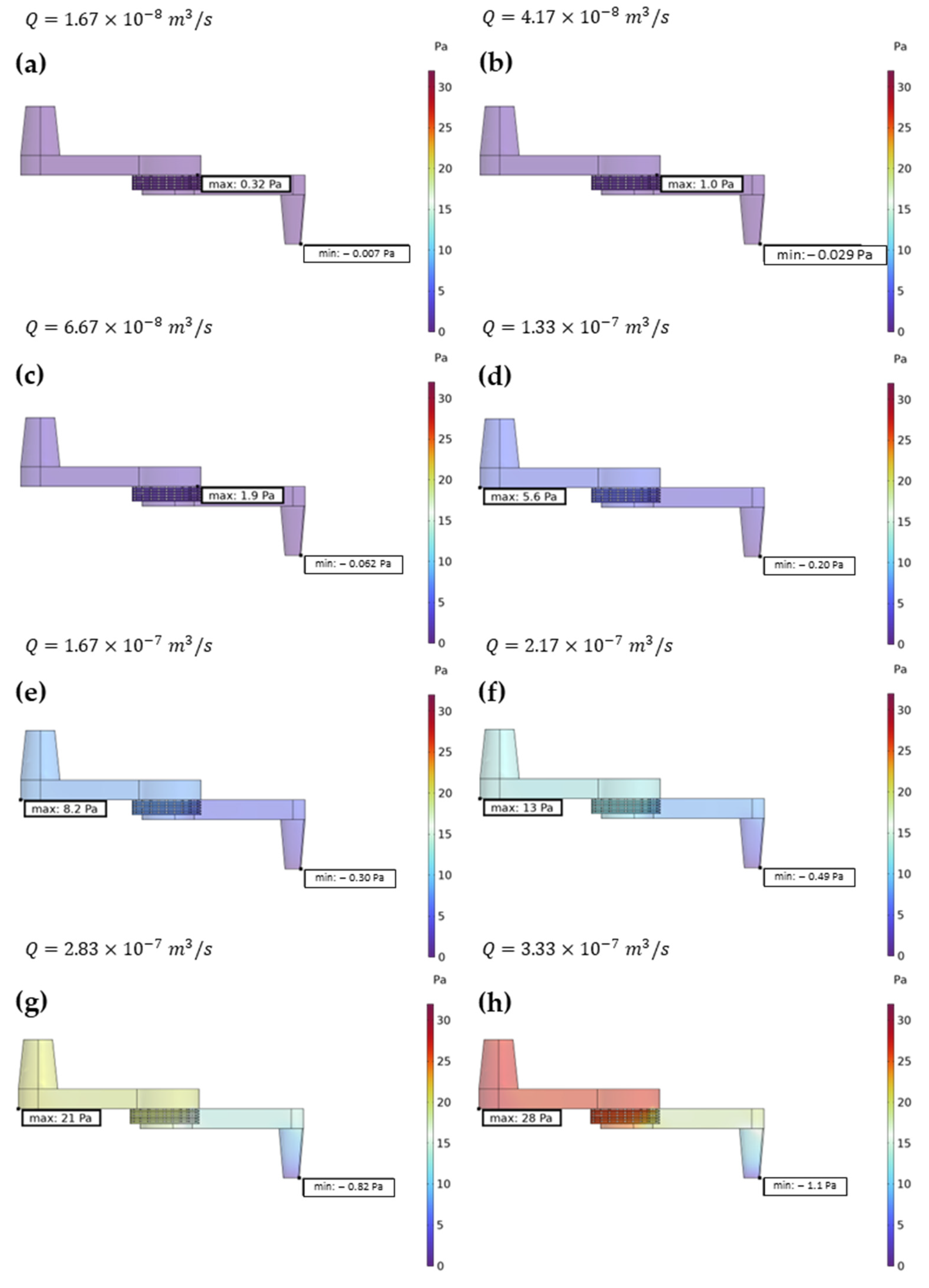
Finite Element Method (FEM) simulations were performed in crucial points of the measuring setup. In particular, the analysis was focused on the detection cell to visualize the flow distribution and velocity all along the external walls, to guarantee high rinsing efficiency between different concentration measures and the filtration system, and to ensure a calibrated pressure drop on the filtering channel, as well as the pressure on the filter itself.

To perform these kinds of simulations, COMSOL Multiphysics (6.1 version) was used with a 3D model and by coupling the Fluid Dynamics and Solid Mechanics modules. As concerns the detection cell, different flow rates of interest were evaluated in the range of 1–20 mL/min in the attempt to define an upper boundary due to pressure on the cell walls. The very same set of flow rates was used in the filtration system. Here, the pressure was analysed both inside the channel, especially on the inlet and outlet surfaces, and on the boundary of the filter. In this specific case, the displacement of the entire structure was also evaluated and taken as a reference parameter for the implementation of the geometry of the system. Since the control parameter was the flow rate through the inlet surface, as a boundary condition, the pressure was considered equal to zero on the outlet of both the filtration system and the detection cell. This was set in order to test the devices, as no connection tubes were attached to the outlet. Therefore, the feedback was the overall pressure drop across the system.

2.2. Chemical Detection

Solutions containing different concentrations of Cr (III) and Cr (VI) were prepared and subjected to UV-Vis spectroscopy analysis to determine the limit of detection (LoD). Calibration curves were constructed for each oxidation state, and the linearity of the system was subsequently assessed. The quality of the spectra and the absorbance peaks were also examined. The prepared samples were analysed using a UV-Vis spectrophotometer (LAMBDATM 35, PerkinElmer, Waltham, MA, USA), employing an optical glass cuvette with a 10 or 20 mm optical path, and compared against pure distilled water as a reference.

Chromium (III) analyses were carried out using two real sample stock solutions of chromium (III) rinsing water from the plastic electroplating industry at different concentrations, namely 0.73 g/L and 7.3 g/L, and these were compared with a commercial high-purity quality chromium (III) chloride hexahydrate powder (Sigma-Aldrich, St. Louis, MO, USA). From the real sample solutions, two set of dilutions were made, from 0.73 g/L to 0.09 g/L and from 7.3 g/L to 0.5 g/L. Samples of distilled water solutions with various concentrations of laboratory standard Cr (III), ranging from 10–0.6 g/L to 0.025–0.003 g/L, were prepared from commercial powder. Vigorous magnetic stirring was employed for higher concentrations, coupled with moderate heating at 40 °C for approximately 8 min to ensure complete salt dissolution in water. It is important to highlight that this sample pre-treatment was solely necessary for the laboratory calibration curve. By contrast, samples derived from the plants could be directly analysed, even at elevated ion concentrations, as the comprehensive salt dissolution was guaranteed by the process parameters.

For the investigation of chromium (VI), a commercially available high-purity standard with a nominal concentration of 1 g/L Cr (VI) in H₂O, designed for ICP analysis (Sigma-Aldrich), was utilized as the stock solution. Dilutions were made to determine the limit of detection (LoD) with respect to maximum and minimum concentrations. Two distinct sets of solutions were prepared, spanning from 100 to 0.5 ppm with a 10 mm optical path length, and from 0.5 to 0.1 ppm with a 20 mm optical length.

To be able to comprehensively assess the quality of the spectra and the precise peak wavelength, a thorough analysis of the solutions was conducted under real-case conditions. The evaluations were carried out at room temperature (RT) and under neutral pH conditions, thereby ensuring the fidelity of the experimental setup to practical scenarios.

2.3. CAD and Fabrication

2.3.1. Filtration System

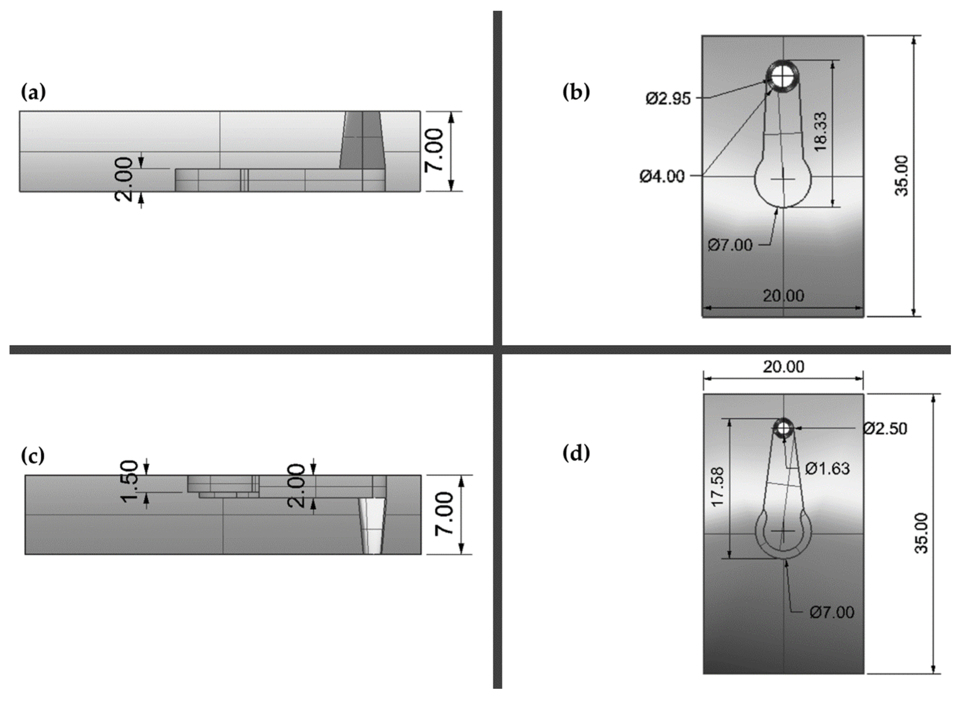
The filtration system was composed of a device with two layers: a top layer with an inlet hole, a channel, and an outlet hole and a bottom layer with an inlet hole that contained the filter housing, a channel, and an outlet hole, as reported in Figure 1. The top layer inlet and the bottom layer outlet were designed respecting the diameter required by the selected system tubes. The filter housing was represented by a little step in the bottom layer inlet that supported the filter and allowed for keeping it in place. This system prevented the passage of particles that could interfere with the detection system.

The device was made of PDMS through the replica moulding technique. PDMS was chosen as the constitutive material for the system because of its mechanical properties, such as strength, durability, tunability of elasticity and viscoelasticity, and channel deformation tunability, with variation in the curing agent concentration [30]. An additive manufacturing technology was used for mould fabrication. They were 3D printed with a PolyJet printer, the Objet30 from Stratasys, using their VeroWhite^TM resin as material. The printed parts were post-processed, eliminating each residue of support material, washing them with water, curing them into the oven (UF30, Memmert GmbH+, Schwabach, Germany) at 110 °C overnight, and cleaning them with acetone in an ultrasonic bath (LBS2, FALC INSTRUMENTS SRL, Treviglio, Italy) for 5 min at 59 kHz [31,32]. Then, the PDMS prepolymer and curing agent (SYLGARD™ 184 Silicone Elastomer kit, provided by Sigma-Aldrich) were mixed with a ratio of 10:1, degassed, and poured into the post-processed moulds. Lastly, the liquid PDMS was cured into the oven at 90 °C for 1 h, and the cured parts were detached from the moulds using isopropanol (IPA).

The filter was 3D printed with a custom-made SL printer (Microla Optoelectronics S.r.l., Chivasso, Italy), using a commercial resin, the Dental Clear from HARZ Labs. The printed geometry is reported in Figure 2, together with the feature dimensions. The 3D printer was equipped with a 405 nm laser, and the selected parameters were 40 mW for laser power and 1500 mm/s for laser speed. After the printing process, the resin residues were washed away with the resin developer (TEK 1969, from KEYTECH solution) in an ultrasonic bath (10 min at 40 kHz); then, distilled water was used for sample cleaning, and, lastly, they were dried with air.

The complete device was assembled using plasma oxygen treatment after PDMS replica washing in ethanol with an ultrasonic bath (5 min at 59 kHz). The plasma parameters, set on the Electronic Diener Plasma Surface Technology machine, were a gas supply period of 1 min, oxygen pressure of 0.7 mbar, and a plasma process duration of 0.30 s at 22% of maximum power. After the plasma treatment, the filter was positioned in the dedicated holes, the two layers were joined together, and a thermal treatment was performed on the bonded layers, using the hot plate (AREC.X, VELP Scientifica, Deer Park, NY, USA) at 80 °C for 5 min to improve the bond.

The assembled device was connected to the monitoring platform system through polytetrafluoroethylene (PTFE) 1/16″ OD tubes, while PTFE 1/8″ OD tubes were selected for the connection with the electrolyte bath.

The PDMS layers and the filters that constituted the filtration system were characterized through digital microscopy; in particular, the VZ80C (Leica, DVM2500 series, Wetzlar, Germany) was used for this work.

The fluidic performances of the assembled device were tested by inserting a solution of water and food dye through a syringe pump. The tested flow rates, limited by the instrument’s restrictions, were 0.05 mL/min, 0.10 mL/min, and 0.15 mL/min.

2.3.2. Monitoring Platform System

The chromium monitoring platform was developed in collaboration with Microla Optoelectronics, which provided electronic and mechanical assets, and it was designed as follows.

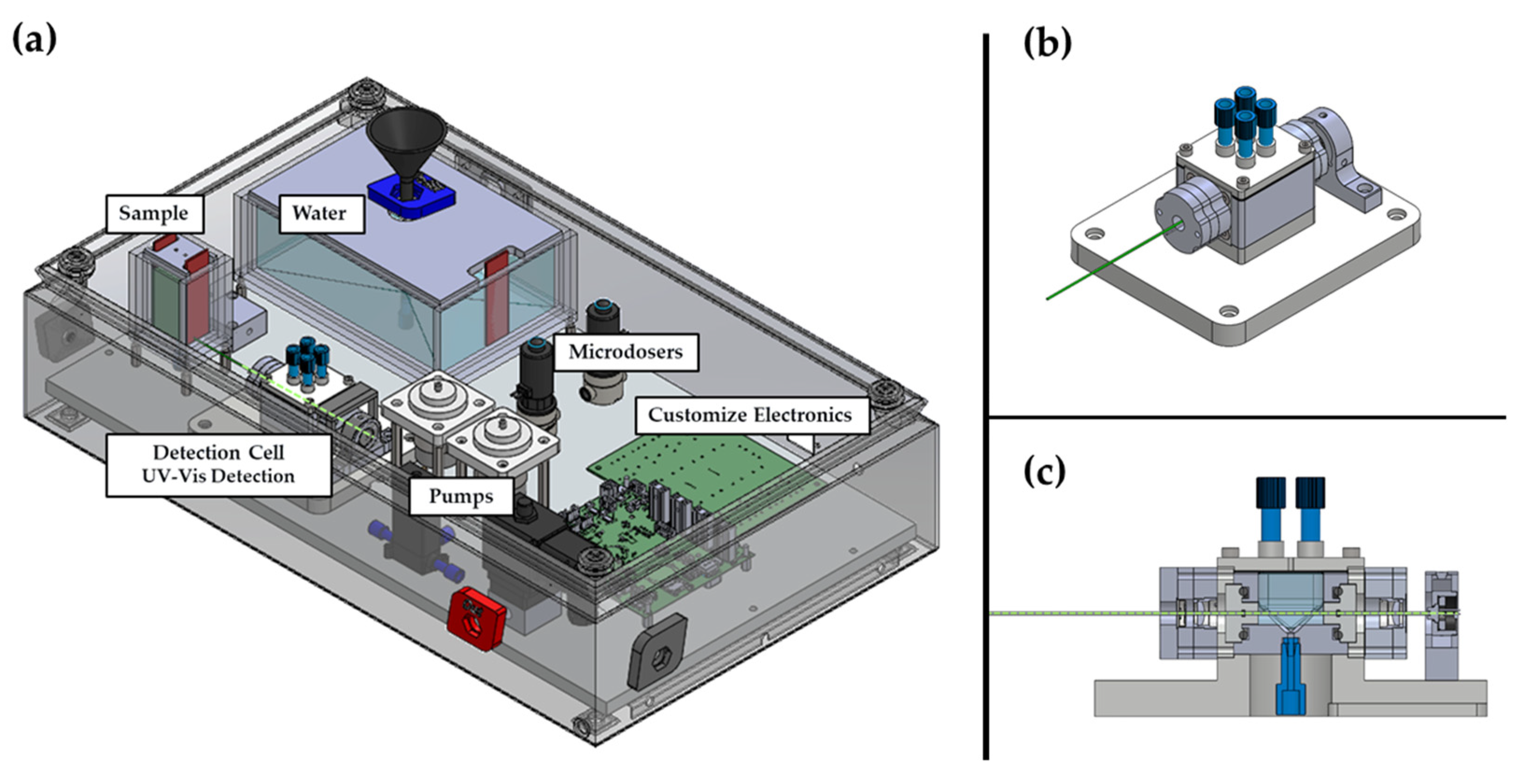
The monitoring platform, described in

Table 1. In situ heavy metal analyser descriptors.

Dimension	Length [mm] Width [mm] Height [mm]	500 300 125
Weight	Weight [kg]	7
Electrical Connection	CEE 7/7	230 V~50 Hz
Communication Port Type	USB Type	B
Inlet Sample	Pressure [bar] PTFE tubes	1.5–5 Ø 1.6 mm
Inlet Ultra-Pure Water	Rilsan® tubes	Ø 8 mm
Outlet Sample	Rilsan® tubes	Ø 4 mm
Waste Sample	Rilsan® tubes	Ø 4 mm

and depicted in Figure 3, included a variety of different components, such as a fully customized electronics system; mechanical parts, such as commercial valves (Buerkert, Huntersville, NC, USA), micro-dosers (SMC, Noblesville, IN, USA), and peristaltic pumps (Fluid-o-Tech, Vista, CA, USA) managing the sample flow; a vast dedicated compartment in Poly(methyl methacrylate) (PMMA) designed for deionized water, serving the dual purpose of referencing in UV-Vis analysis and rinsing the detection cell; a sample holder; and a colorimetric detection cell, where the sample was flowed for UV-Vis spectrophotometric analysis. PTFE tubes 1/16″ OD (Darwin Microfluidics, Gaithersburg, MD, USA) was chosen for sample flow management inside the platform since it showed superior polymer cleanliness. For the management of the outgoing flow, larger tubes in diameter, based on polyamides, were chosen for their superior flexibility and adaptability to external environments. For the UV-Vis monitoring sample cell, aluminium was chosen as the material, and it was cut using a three-axis vertical metal milling machine (RAIS m450). For the final system of detection assembly, a commercial diode (Thorlabs) was mounted at a specific commercial wavelength with respect to the selected analyte under investigation.

3. Results

3.1. FEM Simulation

As concerns the filtering system and the detection cell, eight different flow rates were simulated, ranging from 1 mL/min to 20 mL/min, in particular, 1 mL/min, 2.5 mL/min, 4 mL/min, 8 mL/min, 10 mL/min, 13 mL/min, 17 mL/min, and 20 mL/min. Note that from Figure 4, Figure 5, Figure 6, Figure 7 and Figure 8, SI units are used instead of mL/min.

• Filtering System

Figure 4 shows how the pressure on the filtering system walls evolves while increasing the flow rate. As expected, in all the simulated flow rates, the major pressure drop occurs across the filter and between the filter and the outlet. The first drop is a consequence of the filter geometry that locally reduces the fluid’s cross-sectional area. The second drop is due to the connection with the filtering system and the exit tube, whose geometry represents a convergent nozzle. In this case, the simulation reaches a negative minimum in some spurious points on the outlet surface. The average pressure on the outlet surface is, however, positive. The maximum pressure on the system is 28 Pa, which was detected during the 20 mL/min flow rate simulation.

Figure 5 illustrates the main displacement domains of the filtering system in the specific case of 10 mL/min on the left, and the maximum displacement experienced by the structure as a function of the flow rate on the right. As concerns the left displacement plot, a magnification factor of 20,000 was set to better visualize the displacement with respect to the initial geometry, while the reference colour scale is unaltered. As a result, the part most affected by displacement is the one above the filter, with a net displacement of about $8\times {10}^{-8}$ m. On the right plot, the displacement magnitude as a function of the flow rate is shown. In this plot, the maximum value of displacement, reached with the 20 mL/min flow rate, is about $2.8\times {10}^{-7}$ m.

FEM simulations also allow for better visualizing the streamlines in moving liquids. Figure 6 shows the streamline and liquid velocity across the filtering system for 1 mL/min, 10 mL/min, and 20 mL/min flow rates. As is visible in the three plots, the flow is laminar. Furthermore, as the flow rate increases, the filtering activity becomes more relevant rightwards with respect to the centre of the filter.

• Detection cell:

The objective for the analyte detection cell is to optimize performance and to identify potential limitations. Figure 7 shows the simulation results in terms of pressure. On the left, the pressure on the cell walls in the 10 mL/min flow rate case is shown, while on the right, the pressure difference between inlet and outlet is plotted as a function of the flow rate. The left plot allows for a visualisation of where the pressure drop concentrates the most, which is the final part of the channel towards the outlet. The right plot allows for establishing a relation between the maximum pressure drop and flow rate.

In Figure 8, the streamline plots are shown for each simulated flow rate. As the flow rate increases, many vortices appear all along the cell. Even if the discretisation in terms of the flow rate is not very fine, a threshold appears around 2.5 mL/min. Below that value, vorticity drops, while above that, the fluid reaches any point of the cell. This implies the facilitated and efficient exposure of analytes to the detection zone without generating excessive vortexes, and, consequently, the lack of turbulence improves analytical sensitivity and accuracy.

3.2. UV-Vis Colorimetric Detection

The analysis process for chromium (III) monitoring started with a straightforward yet valuable visual comparison between the two real samples provided. It revealed that, in comparison to the less concentrated solution, the electrolyte sample at 7.3 g/L exhibited a significantly more pronounced and darker green colour. Upon testing the samples of the two solutions, as evident from the spectra presented in Figure 9, it became apparent that the highly concentrated solution rapidly saturated the signal. By contrast, the solution with the lowest analyte concentration of 0.73 g/L exhibited a distinct peak with a maximum wavelength observed at 423 nm. This band is due to the d-d transition of the chromium (III) ion.

To ensure accurate analyte speciation, the identified maximum absorbance wavelength was validated against a standard laboratory dilution series from 10 to 0.6 g/L of Cr (III) prepared under identical conditions (Figure 10). The Cr (III) standard series exhibited a clearly well-defined peak at 425 nm, allowing for the identification of the maximum detectable concentration at 10 g/L. The wavelength of maximum absorbance and its shape remained constant even as the concentration of the chromium (III) solution increased. This indicated that the nature of the absorbing species, as well as the environmental testing conditions, remained consistent across different concentrations. A calibration curve, generated using this standard laboratory series absorbances at 423 nm, exhibited excellent linearity across the studied metal concentrations, confirmed by an R² value approaching 1 (R² = 0.9999). Interestingly, Figure 11 illustrates a difference in absorbance values between the supplied and laboratory samples. In fact, after three recorded spectra at the same concentration, the difference in absorbance can be quantified as ∆ = 0.18 (a.u.).

To calibrate a customized sensor for different real-world concentration scenarios, two sets of dilutions were studied and performed, starting from the provided solutions, as schematically represented in Figure 12. Starting from the less concentrated solution and examining a concentration range from 0.73 to 0.09 g/L, a clear proportionality was observed between the absorbance of the curves and the concentration. This was reflected in an excellent calibration curve, with an R² value close to unity. Performing dilutions from the more concentrated solution and examining a concentration range from 7 to 0.5 g/L, the maximum wavelength remained constant, and the absorbance proportionally decreased from higher to lower concentrations. However, the purple dotted line in the spectra, associated with the maximum investigated concentration, showed some noise, suggesting signal saturation. In fact, the analysis exhibited good linearity for Cr (III) concentrations between 0.5 and 6.3 g/L, as evidenced by the calibration curve shown in Figure 12; however, this registered noise, evidenced by the presence of small spikes, limited the detectability of the upper range to a maximum concentration of 6.3 g/L. This finding is essential for defining the appropriate operational range for accurate measurements.

In order to overcome this LoD limitation using direct UV-Vis spectroscopy, a 1:10 dilution of the most concentrated sample was prepared. The recorded UV-Vis spectra as shown in Figure 13a demonstrated perfect overlap in terms of the maximum wavelength (λ_max = 423 nm) shape of the peak and absorbance. This is essential in the perspective of being able to dilute the more concentrated real sample and to obtain a reliable calibration curve, with comparable and excellent linearity observed for the sample at lower concentrations. Lastly, the time stability of the sample solutions was examined over a two-month period, with a specific emphasis on a 0.73 g/L sample as such and its 1:10 dilution, which exhibited more prominent results for the calibration of a sensor prototype. Figure 13b illustrates how both samples exhibited an absorbance peak at 423 nm that remained constant over time. The diluted sample had a slighter higher absorbance than the undiluted one. After two months, the recorded spectra showed that the variations in absorbance were negligible; however, it is worth noting that the undiluted sample recorded a slightly lower absorbance.

Finally, to expand the domain of the sensor and reach even lower concentrations through a direct UV-Vis method, other analyses were performed, and, as expected, solutions became increasingly transparent to the naked eye as metal concentration decreased. However, the achievement of significantly lower analyte concentration detection was attained by doubling the optical detection path. In fact, the UV-Vis spectra depicted in Figure 14 demonstrates how extending the length from 10 to 20 mm allows for the detection of concentrations down to 0.011 g/L (11 ppm). Importantly, the maximum absorbance wavelength remained constant at 423 nm across both lengths, and the calibration curve depicts outstanding linearity.

At high concentrations, chromium (VI) exhibits a vibrant orange colour. This characteristic makes it an ideal analyte for direct colorimetric detection using UV-Vis spectroscopy. The UV-Vis spectra of a Cr (VI) solution were investigated from 0.015 g/L (150 ppm) to 0.00075 g/L (0.75 ppm); it showed a broad absorption band in the visible region, with a maximum absorbance peak at 349 nm. This band is again associated with the d-d transition of the chromium ion. In the UV-Vis spectra shown in Figure 15, it was observed that the band intensity rose proportionally with respect to the increasing concentration in the chromium (VI) solution. However, as depicted in the magnification, at 100 ppm, the signal began to exhibit some noise, ultimately leading to signal saturation at an analyte concentration of 150 ppm. Due to these observations, the calibration curve did not incorporate these last two concentrations. This yielded excellent results in terms of system linearity, with an R² close to unity.

The LoD for hexavalent chromium using the detection conditions described above was 0.75 ppm. By doubling the optical path length of the analysis, it was also possible to record lower concentrations, still without the use of chromophores, even if the colour of the solutions was no longer visible to the naked eye. As shown in the magnification of Figure 16, a significant increase in absorbance could be observed in the comparison between 10 and 20 mm optical length. For this reason, the decision was made to further record spectra with a concentration range of 0.5, 0.25, and 0.1 ppm. As depicted in Figure 16, the wavelength at which the maximum absorbance was recorded did not change, and a linearity of the system was found, as demonstrated by the excellent calibration curve.

3.3. Filtration System

The microscopy investigation of the PDMS layers, in Figure 17, showed a good agreement between the printed mould and the CAD geometries, confirming that the chosen mould fabrication technology was adequate for the current application.

A digital microscope investigation was also conducted on the SL-printed filter to verify the correspondence between CAD dimensions and the printed object that could undergo volumetric shrinkage phenomena. The microscope images, reported in Figure 18, showed that there was a little shrinkage phenomenon along the Z axes, but the final printed part height was still in line with the fabricated filter step, making the printed part adequate for the entire system.

The fluidic performances, evaluated at three different flow rate values, indicated that the designed system could withstand all the tested flow rates without any deformation.

3.4. Detection Cell

The selection of the laser for the analysis of the system cell was commercially driven by the available diodes on the market. In this sense, the five commercial wavelengths selected are reported in

Table 2. System linearity study for chromium (III) detection with commercial wavelengths.

Commercial Wavelength (nm)	R2 [0.73–0.09 g/L]	R2 [6.3–0.5 g/L]
450	0.9929	0.9875
448	0.993	0.9876
447	0.993	0.9874
445	0.9931	0.9873
405	0.9932	0.9766

; they were chosen because they were the closest to the maximum absorbance value measured in the laboratory. For each of them, the possible linearity value of the system was estimated, considering a lower measurement range from 0.73 g/L to 0.09 g/L and an upper range from 6.3 g/L to 0.5 g/L, which were significant detection ranges. The table shows their excellent linearity even for absorbance values not exactly centred at the peak maximum (this thanks to the broad shape of the signal), and so, each wavelength offered the possibility of functioning effectively. However, after careful evaluation, a laser diode with a package of Ø5.6 mm and a wavelength of 450 nm was ultimately chosen for the detection cell.

A crucial step in establishing the functionality of a homemade in situ monitoring system involved the construction of a calibration curve with the assembled system at a precisely selected commercial wavelength and real sample solutions. This customized curve was subsequently loaded into the system’s software for real-time analysis.

To achieve a full-scale measurement range and to ensure that the system could accurately detect a broad spectrum of concentrations, a systematic dilution process was employed. Starting with a high concentration standard solution of 7.3 g/L, subsequent dilutions were prepared using a dilution factor of 10. The data obtained from these dilutions were then used to construct a five-point calibration curve. This curve correlates the absorbance values measured at a 450 nm wavelength to the known concentrations of the diluted samples. A key performance metric for calibration curves is their linearity factor. In this case, the constructed curve exhibited a linearity factor close to unity (SD = 0.7%, calculated using the Bessel Correction (n − 1)). This indicates a strong linear relationship between the absorbance and the concentration of the analyte, which is essential for accurate quantification within the monitoring system (Figure 19).

4. Discussion

4.1. FEM Simulation

In the design domain of monitoring automatized in situ sensors, the ability to simulate the behaviour of a prototyped device under diverse operating conditions is paramount. This rigorous approach allows for the identification and mitigation of potential shortcomings before and after physical construction; thus, for these reasons, both individual components were studied separately under a wide range of possible working conditions. This broad analysis empowers the optimisation of the outline of each part, ensuring their synergistic operation and, ultimately, the optimal performance of the entire device.

Initially, the parameters necessary to identify the optimal flow rate for both the filtration system and the detection cell were studied. This pursuit of an optimal flow rate offered a significant mechanical advantage in terms of the fluid dynamics of the system. The analytical investigation revealed that a flow rate of 10 mL/min emerged as the optimal choice for both systems and, by maintaining this flow rate, it was possible to minimize pressure fluctuations within the system, ultimately leading to a more robust design. This selection ensured efficient operation while staying comfortably below a predefined flow limit. Notably, exceeding this maximum flow rate presented a specific challenge for the filtration system. At higher flow rates, the pressure within the inlet section would rise significantly, potentially causing damage or even a leak into the chromium sample reservoir. The detection cell, however, presented a different scenario. Although the pressure on the cell walls increased at higher flow rates, the chosen material possessed sufficient mechanical rigidity to withstand these elevated pressures without compromising the system’s integrity. The pressure drop between the inlet and the outlet of the chromium detection cell, observed in the simulation data, serves as indirect validation that the inlet and outlet of the system were appropriately sized.

The analysis of displacement phenomena was confined solely to the PDMS filtration system. The observed displacement was mainly localized above the filter itself. This deformation can likely be attributed to the inherent material properties of PDMS, which exhibits a lower degree of rigidity compared to other potential alternatives. However, the magnitude of this deformation is reassuringly minimal and well within the tolerance, set to $1\times {10}^{-6}$ m, guaranteeing a good coupling capability with the tubes and therefore assuring the seal of the assembly. Crucially, the filter position within the device remains entirely unaffected by any potential displacements from its original position. This validates the selection of the filter printing material and its designated layout.

Finally, streamline plots of both systems were evaluated, allowing for a visualisation and an analysis of flow patterns with respect to different parameters to identify potential issues such as dead zones, recirculation regions, and uneven flow distribution. It also helps to optimize the design of channels, in order to achieve desired flow characteristics, minimizing pressure drops and maximizing efficiency. The simulation results demonstrate that the flow regime within the filtration system is laminar, which ensures a more uniform distribution of the fluid across the entire surface of the filter media, since this characteristic of the device has a high level of efficiency in particle capture; in fact, in laminar flow, possible particles follow well-defined streamlines, minimizing mixing between layers. This allows suspended particles to travel along predictable paths towards the filter media. However, as underlined by the simulation, while the flow rate increases, the filtering activity is shifted rightwards with respect to the centre of the filter. This trend must be carefully considered since the rightwards part of the filter will become more subjected to impurity accumulation. Streamline visualisation within the detection cell served a dual purpose. Firstly, it was employed to meticulously analyse the distribution of the sample across the cell volume. A uniform distribution is fundamental, as it ensures that all analytes within the sample have an equal opportunity to interact with the detection sensors. Secondly, streamline simulations were leveraged to identify the optimal flow rate for effective system washing. Achieving proper washing is necessary to eliminate residual sample or contaminants after analysis, thereby guaranteeing pristine conditions for subsequent measurements. The validation of the 10 mL/min flow rate is reinforced by the observation that the desired outcomes were achieved even at lower flow regimes.

As emphasized by FEM simulation, a trade-off between rapidity in analysis, the stability of the structures that comprise the system, and the pressure, accuracy and sensitivity required by these kinds of measurements, the selection of 10 mL/min as the optimum flow rate is suggested.

4.2. UV-Vis Colorimetric Detection

A combination between UV-Vis technology and colorimetric detection can be used to monitor the concentration and to determine the oxidation state of chromium in a solution.

Due to the straightforwardness of its detection technique, colorimetric methods prove to be highly effective for monitoring high concentrations of various types of heavy metals. Leveraging the UV-Vis principle, namely the Lambert–Beer law, facilitates the establishment of a direct correlation between the colour of the examined solution and the quantification of analyte ions using a calibration curve. In the domain of direct colorimetric detection of a high concentration of pollutants, it is crucial to conduct a meticulous analysis by implementing suitable dilutions. Indeed, upon evaluating the electroplating sample solution, even with the naked eye, it becomes apparent that the most concentrated solution saturates the signal. As evidenced in a previous study conducted by our research group, this approach serves as a pivotal factor in the development of an efficient sensor system [25].

From the comparison between the laboratory-prepared solutions and the provided samples, a finding emerged that indicated that those coming from the plant showed a slightly higher absorbance rate than those recorded from laboratory standard dilutions, causing signal saturation at lower concentrations of 6.3 g/L instead of 10 g/L. This different behaviour may depend on a different composition with respect to a solvent matrix of the analysed solutions in terms of ligands or additives incorporated in the electrolyte process, as well as additional factors, such as pH, that can affect the electronic structure and, consequently, the light absorption properties. Therefore, calibration with the actual sample solution is recommended. However, the peak shape and wavelength remained constant, indicating a high efficiency in detecting the species under examination. Since the most concentrated solution is not directly detectable, dilutions are mandatory to reach the desired range with excellent linearity. Among the dilutions tested, the 1:10 dilution yielded the best results, demonstrating a well-defined peak with excellent overlap. Following these considerations, the calibration of the customized sensor for this detection can be performed directly with the real solutions from the plant after careful dilutions to ensure optimal performance. Additionally, the behaviour of the solution was studied after two months of resting time to ensure sufficiently long system autonomy and minimize maintenance costs. Aside from minor negligible variations, the overlap of the curves indicates good consistency in the recording of the absorbance signal. This observation highlights the outstanding sensitivity of colorimetric detection, and it suggests that the calibration curve initially provided to the system can be maintained for a long period.

Strict and punctual monitoring is advantageous under an industrial point of view, since it is essential for the quality of the final product that the concentration of the electrolytic bath remains constant without variations over time. It is also important for civil purposes to avoid the release of harmful pollutants to the ecosystem and to humans. In this perspective, thanks to the flexibility of the proposed technology, which allows for a broad concentration range from g/L to ppm, the ability to change the optical length to a lower limit of detection was investigated in order to broaden its versatility. Indeed, two optical paths, 10 and 20 mm, were chosen specifically for the purpose of analysis in this study. By modulating the shorter path in depth and the longer path in the length of the proposed colorimetric sensor, the system’s capabilities could be tailored to fulfil diverse analytical needs.

For the online analysis of industrial production processes that require high sampling and analysis frequencies, frequent calibration is crucial to ensure the sensor accuracy and reliability. This is because sensor performance can drift over time due to factors such as exposure to the process’ environment or gradual changes in internal components. To maintain optimal sensor performance and ensure the validity of the collected data, monthly calibration for these high-frequency applications is recommended.

Owing to the effortlessness and efficiency of the employed chemical technique, the capability to detect hexavalent chromium was also implemented. The latter exhibits the same colorimetric characteristics as trivalent chromium, rendering it easily integrable within the sensing platform. Nevertheless, hexavalent chromium is considerably more hazardous to humans and the environment, and its monitoring is far more fundamental. Motivated by the afore-mentioned observation, a similar chemical analysis conducted for chromium trivalent was conducted for hexavalent chromium. Real solutions were not available at that stage; hence, this study involved successive dilutions of standard laboratory solutions. The prepared solutions varied in concentration, reaching a maximum of 750 ppm, which exhibited a very intense orange colour. In this case, the first readable saturation signals on the spectrum were attributable to the 100 ppm of the Cr (VI) solution, rendering the maximum detectable concentration via direct colorimetry 75 ppm. This observation leads to the conclusion that dilutions are necessary for hexavalent chromium before analysis to adapt the system to a real electroplating plant in which high concentrations are employed. Although this may represent an additional step compared to trivalent chromium analysis, it is worth emphasizing that no additional reagents are required, rendering the system safe and requiring less maintenance. The lower LoD levels also demonstrate remarkable adaptability. In fact, by varying the optical length, the signal increased, which allowed the detectable concentration of the analyte under examination to be lowered to 0.1 ppm.

4.3. Filtration System

The provided samples exhibited a non-uniform visual composition due to the presence of small agglomerates. These conglomerates appeared with irregularly shaped particles ranging in sizes of several hundred microns. The cause of their formation has not yet been fully clarified, but it could be due to several factors, including the nature of the starting solution, the process conditions, and the storage history of the samples.

However, the presence of clustered particles posed a significant challenge for the detection system. Due to the small diameter of the tubing used (1/16″ OD), these particles could potentially be transported and cause blockages within the measurement platform.

To address this critical issue and ensure reliable operation, a dedicated filtration system was designed, prototyped, and positioned upstream of the main system. This filtration system effectively blocked agglomerates before they reach the detection zone, preventing any clogging of the tubes and maintaining the integrity of the measurements.

To avoid agglomerate formation inside the tubes before the filtering system, different tubes diameters were chosen, and so, considering the average size of floating particles, ranging from hundreds of µm upwards, 1/8″ OD tubes were selected for the chromium reservoir-filtering system input connection.

As mentioned above, the filtration system showed excellent performance in terms of fluidic behaviour. This success can be attributed, in part, to the meticulously designed inlets and outlets. These features ensured the formation of a reliable seal when connected to the tubes, provided that proper alignment with the corresponding holes was achieved. This emphasis on proper alignment underscores the critical importance of a meticulous system setup for ensuring the optimal operation of the entire device.

The combination between flow rate, determined by simulations, and the diameter of particle size dictated both filter designs in terms of their geometry and material selection. A flow rate of 10 mL/min allows for the selection of compact filter geometries, such as smaller diameter filters, due to the minimal pressure drop at this flow. Furthermore, because of the presence of water as a filtration medium and no chemical reagents involved, selection of the material became less critical. This enabled the exploration of a wider range of filter materials of different pore sizes and geometries. The optimal choice depended on the customizable application and target particle size for achieving the desired filtration efficiency.

4.4. Detection System

Material–sample interactions pose a significant challenge in water quality monitoring, potentially compromising data accuracy and system reliability. To mitigate this risk, all employed materials underwent a rigorous compatibility assessment prior to integration to ensure their resilience and to assess potential interactions between materials and the sample matrix. PTFE tubing stands out due to its unique combination of solvent impermeability and high thermal stability. Aluminium excels in terms of its high mechanical strength and resistance to abrasion, deformation, and chemicals. Pumps and microdosers perform leak-free for a considerable number of measurements, and they were individually calibrated to ensure maximum efficiency in filling the measurement cell.

Reported laboratory studies were conducted using two different concentration ranges to demonstrate the modularity of the system for industrial applications involving high concentrations (g/L) and civil applications involving low concentrations (ppm-ppb). The prototype system was developed following an industrial approach, and, therefore, only the calibration data for the 10 mm optical path length were reported. However, the system versatility can be further extended towards lower concentration ranges. This can be achieved by following a similar approach used for the reported analysis. Here, commercially available wavelengths can be systematically evaluated for their suitability in detecting lower analyte concentrations. By studying the linearity of the system response at these new wavelengths across the desired concentration range, the optimal wavelength for each low-concentration application can be identified and implemented.

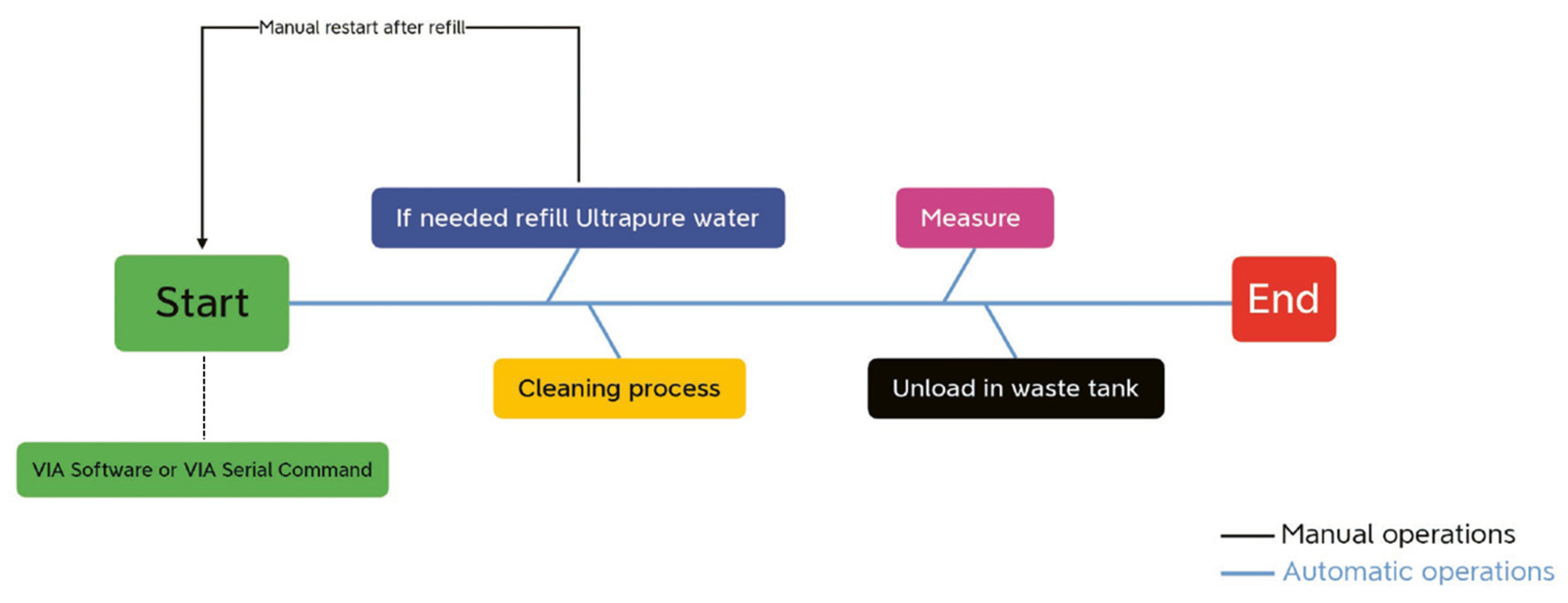
Figure 20 illustrates the automation of the monitoring system described so far. The custom electronics allow the process to be started with a single command, triggering a series of automated steps (represented by the blue line) necessary for measurement once the sample has been loaded into the system. The process begins with a preventive cleaning of the cell, followed by a blank measurement on deionized water. After the ultra-pure water is drained, the sample is charged and measured and then discharged back into the same tank containing the previously used water. Since the volumes involved are small, by adjusting the size of the discharge tank to the work environment, it is possible to obtain a high number of measurements before the waste needs to be disposed of. By now, the only necessary manual process, represented by the black line, is the refilling of the water reservoir. In the absence of deionized water, the system triggers an error notification and returns to the initial start mode, prompting the user to address the issue. This limitation can be overcome in future developments by implementing deionisation systems that connect adequately filtered tap water to the measurement system.

5. Conclusions

The aim of this work is to provide an in situ versatile platform monitoring system able to modulate the detection of chromium in different ranges.

Using the flow rate as a control parameter, very useful insights were determined with FEM simulation, such as the pressure in the filtering system and the optimum flow rate for both the filter and the cell.

The simplicity of the UV-Vis direct colorimetric analysis includes different advantages, such as the absence of chromophores or reagents for the procedure, making this technology well suited for in situ sensing. In particular, the absence of chromophores makes the waste product the same as the input product, making waste management from the analysis identical to process management. The absence of reagents allows for more frequent sampling, as there is no need to plan for their refilling or to ensure a guaranteed time frame after specific analyses that make the reagents reliable for a certain period. It is also worth mentioning that the use of no extra reagents also produces a reduction in the cost of the device and makes it safe for the end user.

The designed filter showed the ability to stop particles whose dimensions ranged from hundreds of µm upwards, effectively protecting the platform system. The device is also cost-effective due to the simplicity and speed of the additive manufacturing technique used to produce it. Moreover, it also exhibited a great capability to be cleaned in an easy and green way by flowing clean water in the opposite direction and collecting the residues suspended in the water at the inlet hole. Future efforts will be directed towards refining the cleaning process to optimize system reusability, leading to significant cost reductions in filter fabrication and waste management.

The successful development of the described versatile online platform monitoring system holds significant promise for various applications, including industrial process control, environmental monitoring, and public health protection.