Groundwater Sustainability and Land Subsidence in California’s Central Valley

Abstract

The Central Valley of California is one of the most prolific agricultural regions in the world. Agriculture is reliant on the conjunctive use of surface-water and groundwater. The lack of available surface-water and land-use changes have led to pumping-induced groundwater-level and storage declines, land subsidence, changes to streamflow and the environment, and the degradation of water quality. As a result, in part, the Sustainable Groundwater Management Act (SGMA) was developed. An examination of the components of SGMA and contextualizing regional model applications within the SGMA framework was undertaken to better understand and quantify many of the components of SGMA. Specifically, the U.S. Geological Survey (USGS) updated the Central Valley Hydrologic Model (CVHM) to assess hydrologic system responses to climatic variation, surface-water availability, land-use changes, and groundwater pumping. MODFLOW-OWHM has been enhanced to simulate the timing of land subsidence and attribute its inelastic and elastic portions. In addition to extending CVHM through 2019, the new version, CVHM2, includes several enhancements as follows: managed aquifer recharge (MAR), pumping with multi-aquifer wells, inflows from ungauged watersheds, and more detailed water-balance subregions, streamflow network, diversions, tile drains, land use, aquifer properties, and groundwater level and land subsidence observations. Combined with historical approximations, CVHM2 estimates approximately 158 km³ of storage loss in the Central Valley from pre-development to 2019. About 15% of the total storage loss is permanent loss of storage from subsidence that has caused damage to infrastructure. Climate extremes will likely complicate the efforts of water managers to store more water in the ground. CVHM2 can provide data in the form of aggregated input datasets, simulate climatic variations and changes, land-use changes or water management scenarios, and resulting changes in groundwater levels, storage, and land subsidence to assist decision-makers in the conjunctive management of water supplies.

1. Introduction and Background

Water scarcity can be a significant threat to global food supplies [1]. Groundwater provides nearly 50% of the water used for global food production [2,3]. This reliance on groundwater can create imbalances in groundwater budgets and cause severe declines in groundwater levels and groundwater storage depletion [1,4,5]. California is the most populated of the United States and the fifth largest agricultural producer in the world, with more than USD 50 billion in agricultural cash receipts in 2019; therefore, water scarcity issues are particularly concerning for California. Similar to global use, groundwater provides about 40 percent of water use in California [2,3]. In California, increasing trends in the consumptive use caused by agricultural and urban development and climate-induced changes in water budgets threaten the sustainability of groundwater supplies.

Integrated hydrologic models provide water managers with the tools required to predict and assess changing conditions (e.g., climate, surface-water delivery, and land use) and the outcomes of possible alternate water-management approaches. Models are often the foundation on which to build effective water management strategies and are the tool used for compliance with California’s Sustainable Groundwater Management Act (SGMA). The goal of this paper is to provide an integrated overview of groundwater availability and sustainability in California, particularly the Central Valley, in which sustainability is particularly concerning. To quantify sustainability in the Central Valley, a broad overview of the history of water use and SGMA is given, and an updated Central Valley Hydrologic Model (CVHM) [5] is used to quantify the sustainability of groundwater resources in the Central Valley. In this paper, CVHM is used to refer to the generic components that are consistent for both versions of the CVHM. CVHM1 or CVHM2 are specified when the context is specific to a particular version. This manuscript’s Supplementary Material provides details on the updates to CVHM2. Briefly, CVHM2 simulates the timing of land subsidence more accurately by incorporating effects that delay deformation, the separation of the inelastic and elastic portions of land subsidence, an updated texture model, inflow from small watersheds and mountain-front recharge, more detailed well construction for inter-borehole flow, and the inclusion of recharge from water banks.

1.1. California Water Supply

California’s climate is volatile and varies spatially and temporally. California receives about 75% of its rain and snow in montane watersheds north of Sacramento. However, 80% of California’s human water demand originates from the southern two-thirds of the state [6], particularly the southern portion of the Central Valley. Water budgets and trends in water supply are dependent on human demands that are superimposed onto ecosystem demands and are not accurately captured for all or even most of the ecosystem for various reasons. Precipitation and streamflow vary significantly from year to year [7,8]. California has experienced large variations between dry and wet climatic patterns. Changes in climate result in longer and more frequent hotter and drier periods, reduced snowpack, and drier soils, which make California’s water supplies more vulnerable to depletion [7,9,10]. California’s population of over 39 million people (according to 2020 Census Bureau estimates [11]), expansive agriculture, and environmental flow requirements increase pressure on its aging water infrastructure, which provides surface-water and groundwater through wells, canals, and rivers. Water stored during the wet winter and spring months (typically October through March, though in recent years, the wet season has often been delayed and shorter) in snowpacks and reservoirs provide storage to sustain demand during dry summers and frequent droughts. Because of the spatial and temporal variability of surface-water, California’s water system includes a vast infrastructure to move water from source areas to demand areas. The State Water Project (SWP) redistributes water from northern California’s rivers to the Central Valley, southern California, and the San Francisco Bay area using a network of reservoirs, canals, and other infrastructure, including the Governor Edmund G Brown California Aqueduct [6]. The Federal Central Valley Project (CVP), operated by the Bureau of Reclamation, consists of multiple reservoirs, canals, hydroelectric power plants, and other facilities [6]. Part of the CVP is the Delta–Mendota Canal, a 188 km long aqueduct that runs southward along the western edge of the San Joaquin Valley and empties into Mendota Pool on the San Joaquin River after supplying water to meet urban and agricultural demands (Figure 1). The Friant-Kern Canal, a 245 km-long aqueduct located on the east side of the San Joaquin Valley [2], is also part of the CVP and supplies water to the eastern Tulare Basin. Despite decreases in deliveries due to drought, the conveyance is often a bigger restriction on water delivery [12], and operational changes may also be needed to improve the resilience of the system to a more volatile climate [2].

Groundwater, although largely invisible, is the largest source of storage in California’s water system [6]. The amount of water supplied by groundwater fluctuates with the large annual and interannual variations in precipitation that substantially affect snowpack, surface-water, and groundwater storage [5,7,9,10]. About 85% of Californians depend on groundwater for some portion of their water supply [12], and groundwater is a critical resource for agriculture, particularly in the Central Valley. In this century, drier conditions and environmental flow requirements have reduced the volume of surface-water available and increased groundwater use for public consumption and agricultural use [5]. Groundwater is often used as a buffer when surface-water supplies are low, such as in dry periods or droughts. In non-drought years, groundwater comprises about 33% of the total water used for consumptive use, but during severe droughts, groundwater comprises more than 50% of the total water used [5]. Groundwater contributes substantially to the flow of rivers, which resource managers allocate to maintain environmental flow requirements in rivers [5]. Groundwater resources allow water managers flexibility in the more extreme drought and floods that California is experiencing and that are predicted to intensify. Changes in climate and less snow in the Sierra Nevada [13] will likely decrease the surface-water available for agriculture and further increase stress on groundwater resources. More than a century of groundwater depletion has created storage space in aquifers that can be replenished, albeit at a slower rate than surface reservoirs.

1.2. Sustainable Groundwater Management Act (SGMA)

Historically, landowners largely controlled the use of groundwater resources. However, declining groundwater levels, drying wells, the permanent loss of groundwater and storage capacity, and land subsidence [2,14] have led to the development of the Local Groundwater Management Assistance Act of 2000 (Assembly Bill 303) and the adjudication of groundwater rights in certain basins [2] to regulate groundwater use. In 2014, California adopted the Sustainable Groundwater Management Act (SGMA) to help manage groundwater resources [15]. The SGMA aimed to address the impact of the compounding of decades of overuse and droughts on groundwater supplies. The SGMA originally applied to 127 of 515 total basins, designated as either high- or medium-priority basins (Figure 1), which accounted for an estimated 96% of annual pumping in California and 88% of the population within high- and medium-priority basins [15]. The SGMA consists of three bills that are likely to have long-term and substantial impacts on California’s economy, agriculture industry, rural communities, and wetlands [15]. Based on stipulations in the SGMA, local Groundwater Sustainability Agencies (GSAs) were formed for all high- and medium-priority basins in California. These GSAs developed and submitted Groundwater Sustainability Plans (GSPs) for managing and using groundwater without causing the following “sustainability indicators” (also referred to as “undesirable results”):

• Groundwater-level declines;
• Groundwater storage reductions;
• Seawater intrusion;
• Water-quality degradation;
• Land subsidence;
• Interconnected surface-water depletions.

Figure 1. Map of California’s Sustainable Groundwater Management Act (SGMA) Basin prioritization [16] and extent of the four Central Valley Hydrologic Model (CVHM) regions (identified by the surface-water basin) and twenty-one Water Balance Subregions (WBSs) [5]. Hydrograph and subsidograph locations are identified and numbered according to their location in the rectangular system for the subdivision of public land.

Figure 1. Map of California’s Sustainable Groundwater Management Act (SGMA) Basin prioritization [16] and extent of the four Central Valley Hydrologic Model (CVHM) regions (identified by the surface-water basin) and twenty-one Water Balance Subregions (WBSs) [5]. Hydrograph and subsidograph locations are identified and numbered according to their location in the rectangular system for the subdivision of public land.

GSPs are designed to reach sustainability by 2040, and the sustainability indicators cannot exceed their 2014 estimates established in the GSPs. However, GSPs and their implementation are subject to review and approval by the state and are reassessed every five years. Initially, more than 260 GSAs were formed for areas covering more than 140 of California’s groundwater basins (inclusive of the 127 high- and medium-priority basins), 21 of which are critically over-drafted, of which 11 are in the Central Valley (Figure 1). A crucial part of the SGMA is that local GSAs are each allowed to develop their own plans for achieving sustainable groundwater use, allowing for flexibility to implement water-management strategies that make sense on a local scale. GSPs across the state include a variety of supply and demand management strategies. In many areas, sustainability likely cannot be achieved solely by supplementing supplies. The SGMA allows basins to reach sustainability over two decades, but the SGMA was passed almost a decade ago, and in many areas, particularly the San Joaquin Valley, there have been little, if any, demonstrable improvements with respect to the sustainability indicators [2]. As the SGMA continues to be implemented, the San Joaquin Valley will likely need to adapt to a future with less water available for irrigation [12], and land uses in the San Joaquin Valley will likely have to change to meet GSP goals. SGMA and its companion legislation have increased the availability and diversity of data accessible to monitor and measure groundwater.

1.3. California’s Central Valley

California is like many semi-arid agricultural regions around the world that rely on groundwater for irrigation [17]. California’s agriculture relies on the conjunctive use of federal, state, and local water systems that divert surface-water from streams and canals and pump groundwater to supply agricultural fields. Twenty-one high-priority basins, 11 of which are categorized as critically over-drafted, are within California’s Central Valley (Figure 1). On average, half of the groundwater in California is pumped from the Central Valley groundwater basins [2]. During periods of drought, groundwater provides 67% or more of the Central Valley’s irrigation water [2,5]. Over the past few decades, droughts and below-average precipitation have reduced surface-water reliability in the Central Valley [5,18,19], leading to increases in groundwater use and groundwater storage depletion. Groundwater storage depletion has caused several other issues, such as land subsidence [14,20,21,22], water quality degradation [23,24], the loss of groundwater-dependent ecosystems, reductions in stream base flow [25], and increasing pumping costs due to groundwater-level declines [5,26]. Groundwater pumped out of the Central Valley results in most of the storage losses and land subsidence in California. Hence, the overall success of the SGMA largely depends on Central Valley GSAs mitigating the sustainability indicators outlined in the SGMA.

California’s Central Valley covers about 52,000 km² and is dominated by irrigated agriculture (Figure 1, Figures S1 and S3) [5]. Roughly 80 km in width and 640 km in length, the Central Valley is drained by the Sacramento and San Joaquin Rivers and can be divided into two large parts: the northern one-third is the Sacramento Valley, and the southern two-thirds are the San Joaquin Valley, which is composed of the San Joaquin and Tulare Basins. The Tulare Basin is internally drained and periodically forms Tulare Lake. The San Joaquin and Sacramento Valleys meet in the Sacramento–San Joaquin Delta and discharge to the Pacific Ocean. Most of the Central Valley is close to sea level and has very low relief.

In the Central Valley, agriculture is the dominant land use, and land-use changes have occurred both gradually and rapidly in response to changes in climate, urbanization, agricultural methods, and economics [2,5]. Irrigated agricultural acreage increased almost linearly starting in the 1940s through to the early 1980s, after which total acreage have fluctuated [2,5]. Since the early 1980s, irrigated acreage has remained relatively stable [27,28,29], and most crop types remained essentially unchanged between the early 1960s and early to mid-1990s. From the 1960s through to the mid-2000s, irrigated crop acreage declined with fallowing during drought.

The compilation of reported acreage for crops on a yearly basis between 2000 and 2013 allowed for a more detailed analysis of land-use trends (Figure S3b) [29]. Land-use data by county indicated that the total acreage for fruits and nuts increased by about 40%, while field and grain crops declined comparably, especially regarding cotton. Cotton decreased by about 70% between 2000 and 2013 because it was replaced by more profitable crops, such as perennial fruits and nuts (tree or vineyard) [2,29]. Historically, cotton has been one of the most important crops in the Central Valley—with over 4050 km² planted in the early 1990s. However, less than 1000 square kilometers of cotton remained in 2018 and 2019 (Figure S3). Perennial fruit and nut acreage has nearly tripled from the mid-1970s to the late 2010s and accounted for roughly 60% of irrigated crop acreage in the 2010s [2,28,29,30]. The San Joaquin Valley contains a diverse mix of crops, but perennials represented more than 50% of agricultural acreage (irrigated crop acreage from [12,28,31]) in 2019 (Figure S3). Changes in planted crops are largely driven by market demand but also demonstrate changes in water availability (Figure S3b).

Changes in crop acreage and types can substantially impact water use and irrigation return flow. Some croplands, particularly non-permanent crops in the western and southern Central Valley, are fallowed during dryer years (Figure S3). Water demand increases dramatically when crops with lower water requirements are replaced by crops with higher water requirements, such as when field and grain crops are replaced by perennials (fruits and nuts) [14,32]. In addition, the value of the established perennial is considered when facing water shortages, and the cost of idling or fallowing a permanent crop is extremely high, which can increase water demand.

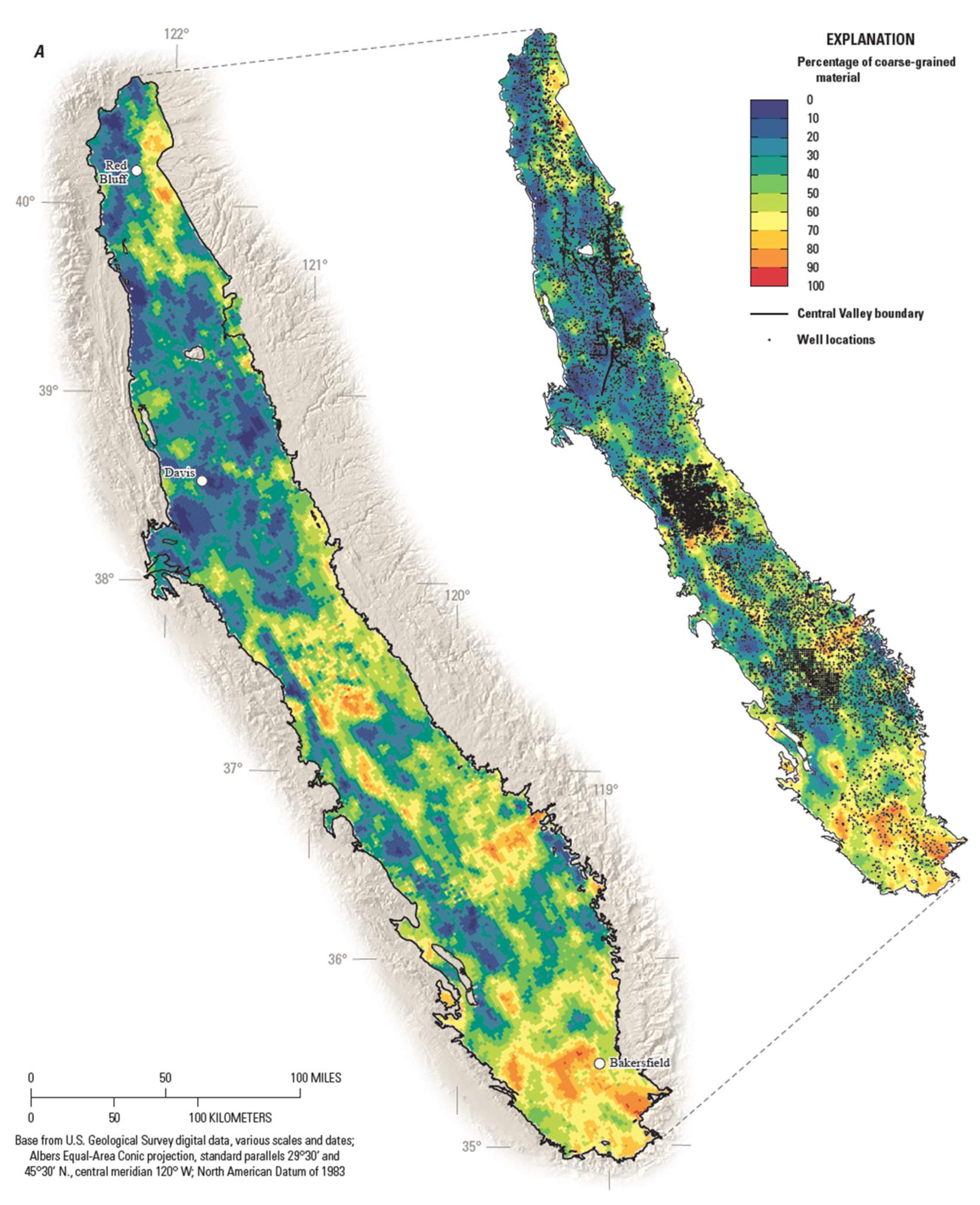
2. Central Valley Geology and Texture

The Central Valley is an asymmetric structural trough filled with sediments as deep as 5 km in the San Joaquin Valley and as much as 10 km deep in the Sacramento Valley. However, most of the freshwater is contained in the upper part of the sediments [22], with thicknesses ranging from 300 to 900 m. During the recent droughts, well drilling increased, and deeper wells were drilled. As a result, since the publication of CVHM1, many new well logs have been available and digitized [33]. To characterize the aquifer-system deposits, we compiled and analyzed lithologic data from approximately 15,000 drillers’ logs of boreholes ranging in depth from 3 to 2227 m below the land’s surface (Figure 2 and Figure S6) [34]. The logs corroborate and refine previous observations of aquifer-system sediments comprising heterogeneous mixtures of unconsolidated to semi-consolidated gravel, sand, silt, and clay (Figure 2).

Based on the methods defined by [34], the three-dimensional (3-D) texture model was updated [33]. The lithologic descriptions on the logs were simplified into a binary classification of coarse- or fine-grained material. The percentage of the coarse-grained sediment, or texture, was then computed from this classification for each 15 m depth interval of the drillers’ logs. A 3-D texture model was developed for the basin-fill deposits of the Central Valley by interpolating the percentage of coarse-grained deposits onto a 2.6 km² spatial grid at 15 m depth intervals from the land’s surface to 550 m below the land surface, which is the depth chosen to represent the depth to the base of freshwater and the deepest wells in the San Joaquin Valley [34].

The 3-D texture model shows substantial heterogeneity and systematic variation in the texture of the sediments [34] (Figure 2). The drillers’ logs and resulting texture model have alternating layers of coarse- and fine-grained materials. Coarse-grained deposits comprise approximately 30% of the aquifer system, which means that the Central Valley aquifer system is composed of about 70% fine-grained deposits dominated by silt and clay beds. These silts and clays make the aquifer system confined to semi-confined. Although these fine-grained lenticular deposits are discontinuous, they are distributed throughout the stratigraphic section, significantly impeding vertical groundwater flow. The 3-D texture correlates well with depositional source areas, independently mapped geomorphic provinces, and factors affecting the development of alluvial fans (Figure 2). In general, the Sacramento Valley is predominantly fine-grained and is composed of volcanic-derived sediments. However, some relatively coarse-grained deposits occur along the river channels and the alluvial fans.

In the San Joaquin Valley, especially on the eastern side, the areas of coarse-grained texture are more widespread than the areas of fine-grained texture and occur along the major rivers and their associated alluvial fans. In the southern part of the San Joaquin Valley, the alluvial fans derived from the glaciated parts of the Sierra Nevada are much more coarser-grained than the alluvial fans to the north (Figure 2). In contrast to the eastern San Joaquin Valley, the western San Joaquin Valley generally is finer-grained and is underlain by the Corcoran Clay Member of the Tulare Formation (hereafter referred to as the Corcoran Clay) (Figure 2).

With the SGMA and the heightened importance of understanding land subsidence and storage change, the accurate distribution of textural properties becomes more important. The airborne electromagnetic (AEM) method can be used to map the large-scale structure of the groundwater systems of the Central Valley [35,36]. The AEM method is a helicopter-deployed system that acquires data along planned flight lines to measure the electrical resistivity of the subsurface to depths of approximately 300 m. Through calibration with drillers’ logs data, electrical resistivity values are then transformed into texture, e.g., sand, gravel, silt, and clay. In particular, AEM data provide information about the abundance of electrically conductive clays and the continuity of extensive clays, such as the Corcoran Clay, which is challenging to capture in the drillers’ log data. Because AEM is a cost-effective way to acquire the lithology or texture data of aquifer systems [35], the state collected and released AEM data for the Central Valley and throughout California’s high- and medium-priority groundwater basins [37].

Although AEM data are available, using them can be challenging because different models are needed in different areas and at different depths to help translate the resistivity information into a metric that can be used to define hydraulic properties. Storage properties and differences between horizontal and vertical conductivities need to be accurately assessed. Interpretations require the inversion of the data and calibration through “models”. To transform the resistivity models, the relationship between resistivity and lithology is established using collocated lithology logs (from drillers’ logs). In addition, water quality greatly affects the ability to interpret these data because AEM models can mistake conductive “salty” waters as fine-grained materials and cannot be used in urban or agricultural areas where there is a potential for interference due to high concentrations of metal infrastructure. Although these data are improvements on mathematical interpolations between borehole data, care must be taken in using and interpreting this information. However, previous researchers [35] demonstrated that AEM can be an effective method for mapping the large-scale texture of aquifer systems like the Central Valley. In a recent AEM application in the Central Valley, the interpretation of lithology was consistent with other lithologic information from the area; however, the AEM method resulted in an overestimation of the thickness of the Corcoran Clay and an inability to detect relatively thin layers at depth [35]. Despite these shortcomings, AEM is a source of surrogate information on hydraulic properties for a wide variety of uses. However, AEM data were not available in time to directly incorporate them into either version of CVHM.

3. Central Valley Hydrologic Model (CVHM)

Integrated hydrologic models can predict and assess changing conditions (e.g., climate, surface-water delivery, and land use) and the outcomes of possible alternate water-management approaches [5,15,38,39,40]. These models provide water managers with diagnostic tools to estimate historical subsidence, predict future subsidence, analyze the effects of projected future conditions, and evaluate a variety of groundwater management strategies. Models are often the foundation on which to build effective water management strategies and are central to the majority of GSPs, particularly those in the Central Valley [5,15,38,39,40]. Often, the challenge faced throughout California is the lack of adequate information about water use and the subsurface characteristics to use as the basis for model development. SGMA and companion legislation are serving as a tool to address these challenges at local and regional scales.

The California Central Valley Groundwater-Surface-Water Simulation Model (C2VSim) [38] and the Central Valley Hydrologic Model (CVHM) [5,14] are regional models developed to simulate the integrated hydrologic system in California’s Central Valley. Both models often use and report temporal information by water year (WY). A WY is the period from October 1 through to the following September 30 and is named for the year in which the period ends. For simplicity, WYs are used in this paper. Coarse-grid (C2VSimCG) [41] and fine-grid (C2VSimFG) [42] versions of C2VSim were developed and are maintained by the California Department of Water Resources (CDWRs) and simulate water years 1973 through 2015. C2VSim simulates the groundwater system but is more focused on simulating the surface-water, soils, and agricultural parts of the system [38]. During the upgrade of CVHM1 to CVHM2, inputs and outputs from C2VSim and CVHM were analyzed to improve both models.

The CVHM [5,29,33,43,44,45,46,47,48,49] is an integrated hydrologic model built to understand and quantify groundwater storage and land subsidence on a regional basis. CVHM1 simulates the water years 1962 through 2003, while CVHM2 extends the period and simulates water years 1962 through 2019. CVHM was developed by the USGS using a specialized version of MODFLOW [50,51] called the MODFLOW One-Water Hydrologic Flow Model (MODFLOW-OWHM, [52,53]). MODFLOW-OWHM combines the hydrological processes of groundwater flow, surface-water flow, landscape and agricultural processes, aquifer compaction, and land subsidence within a single simulation framework. By merging and enhancing multiple specialized versions of MODFLOW-2005 [50], MODFLOW-OWHM provides a comprehensive tool for analyzing conjunctive-use management and addressing water-use and sustainability challenges. In MODFLOW-OWHM, the Farm Process (FMP) (appendices 4, 5, and 6 in [53]) dynamically allocates groundwater recharge and groundwater pumping based on crop water demand, surface-water deliveries, and depth to the water table. More detailed information on MODFLOW-OWHM can be found in [53].

CVHM2 focuses on groundwater availability and land subsidence in the Central Valley. CVHM2 simulates the water years 1962 through 2019 on a monthly stress period (two-week time step). CVHM2 has 2.6 km² cells and is discretized vertically into 13 layers ranging in thickness from 3 to 550 m (Figure S5). The upper three layers from the CVHM1 are split into five layers, the Corcoran Clay that was previously simulated as two layers are split into three, and the lowest 5 layers of the CVHM2 correspond to the original lowest five layers in the CVHM1 (Figure S5). Groundwater pumping for irrigation historically has not been metered; therefore, the FMP automatically pumps groundwater that supplements surface-water to meet the irrigation demand. CVHM2 simulates un-metered historical pumping and the delivery of surface-water for 135 water balance subregions (WBSs or farms) within the Central Valley (Figure S1). The original 21 WBSs from CVHM1 were disaggregated in the Sacramento–San Joaquin Delta and along the Delta–Mendota Canal to better understand the spatial and temporal distribution of land subsidence in this region and to include managed aquifer recharge (MAR) facilities in other areas of the San Joaquin Valley (Figure S2). As in CVHM1, for analysis, 135 farms were aggregated to the 21 WBSs and, at times, these were further aggregated to 4 regions referred to as the Sacramento region, Delta–Eastside Streams region, San Joaquin Basin region, and Tulare Basin region (Figure 1, note: basins are based on surface-water basins (Supplementary Material)). The farm delivery requirement (irrigation requirement) is calculated from consumptive use (calculated in MODFLOW-OWHM from the crop coefficient and reference evapotranspiration), effective precipitation, groundwater uptake by plants, and on-farm efficiency. The details of the farm delivery requirements are described in [5].

CVHM2 simulates groundwater and surface-water flow, irrigated agriculture, land subsidence, and other key processes in the Central Valley on a monthly stress period (two-week time step). The texture model from CVHM1 was updated and used to estimate hydraulic conductivity for every cell in the model [33]. Intra-borehole flow, an important mechanism for vertical flow within and between hydrogeologic units in parts of the valley, is simulated throughout the domain using MODFLOW’s MNW2 Package [54,55]. Relative to the amount of pumping, inter-borehole flow is small, with <5% of the annual pumping, but twice as much during wet years than dry years and much larger across the Corcoran Clay than the other layers. Flux from the surrounding mountains (mountain-block recharge) was estimated with the Basin Characterization Model (BCM; [56]) and is simulated using MODFLOW’s WEL Package [50,57]. Net flux in and out through the delta is simulated using MODFLOW’s GHB Package [50]. Land subsidence, a consequence of intense groundwater pumping in susceptible aquifer systems like the San Joaquin Valley, is simulated using MODFLOW’s SUB Package [51,53]. In CVHM2, compaction and, ultimately, land subsidence are simulated using a hybrid approach with compaction from delay and non-delay clay interbeds. The term delay refers to the slow draining of thicker clay beds, resulting in a delay in compaction that can last for hundreds of years [58]. In some locations, the magnitude of storage changes, and land subsidence varies greatly throughout short distances (horizontally and vertically). More details on model development and calibration strategies are described in [5]. Details on updates from CVHM1 to CVHM2 can be found in this manuscript’s Supplementary Materials.

4. Enhancements and Limitations

The CVHM2 includes significant technical enhancements from CVHM1 to comprehensively simulate the groundwater system and data enhancements to bring the model and the underlying datasets closer to present conditions (especially given the recent extreme droughts and flood events). Enhancements include adding water-banking data, simulating pumping with multi-aquifer wells and at actual well locations for urban and domestic pumping, adding inflows from ungauged watersheds, and extending the simulation period through to 2019. In addition, the more broadly available groundwater level and land subsidence monitoring data associated with California’s SGMA, more detailed water balance subregions, and more detailed diversions from the Delta–Mendota Canal have allowed CVHM2 to simulate land subsidence and storage changes more robustly. The details of the enhancements included in CVHM2 are found in the associated data releases [29,33,43,44,45,46,47,48,49,59] and the manuscript’s Supplementary Material. Many enhancements are focused on improving the accuracy of land-subsidence simulations.

Like CVHM1, our goal in developing CVHM2 was to provide a model capable of being accurate at scales relevant to water-management decisions. CVHM2 was designed to portray general characteristics for examining hydrology at a regional scale; CVHM2 was not designed to reproduce every detail of the Central Valley hydrologic system. For example, the scale of the spatial distribution of deliveries used in the CVHM2 is regional to subregional in scale. If deliveries are used in greater spatial detail, groundwater pumping could be estimated in greater spatial detail. Despite the limitations, CVHM2 is designed to facilitate the addition of more detailed features that may be relevant at a more local scale, such as the sub-regional to GSA scale. CVHM2 uses the latest datasets and modeling methods available, but there are inherent limitations associated with the use of numerical models to simulate hydrologic systems. Limitations of the modeling software, data limitations, assumptions made during model development, conceptual model error, and the results of model calibration and sensitivity analysis all are factors that constrain the appropriate use of the CVHM. The details on the limitations of CVHM1 are still applicable and described in [5]. Although CHVM2 does include more detailed accounting units, particularly along the Delta–Mendota Canal, these details are not always easily available through time for the entire Central Valley. Given these limitations, the CVHM2 can be used to represent the longer-term changes and larger spatial trends in groundwater storage and can simulate regional and sub-regional groundwater flow and land subsidence.

Calibration

The CVHM (both versions) simulates the long-term trends in hydrologic conditions and water use in the Central Valley. The overall calibration methods for CVHM2 are similar to methods used to calibrate CVHM1 [5]; the model was recalibrated by adjusting hydraulic and land-use parameters to better match the simulated results with observed datasets (field measurements). CVHM2 uses CVHM1 parameters as a starting point; however, the CVHM2 parameterization was more extensive than CVHM1 because CVHM2 simulates a more detailed hydrologic process and often leverages enhanced packages and processes in MODFLOW-OWHM and includes a more detailed aquifer texture model. This section provides a high-level overview of the CVHM2 recalibration, and further details on the model calibration methods and results are provided in [5] and the Supplementary Material associated with this manuscript.

Like CVHM1, the degree to which the CVHM2 simulation provides a reasonable representation of the hydrologic system was evaluated by comparing simulated hydrologic conditions with observed field conditions. Observed datasets used in the CVHM2 calibration built upon the datasets used in CVHM1 included groundwater level and change in groundwater levels (drawdowns and trends), land subsidence and compaction, streamflow, and drain flow [46]. CVHM2 generally replicated, complemented, and extended results from previous studies of water availability in the Central Valley [5,22,38,42]. The final calibrated model produced simulated results that reasonably matched the more than 300,000 observations. The observations include groundwater levels, changes in groundwater levels, relative land-surface altitude and compaction, and streamflow and drain flow (Supplementary Material and [5]). The calibrated model was used to estimate parameter sensitivity and demonstrated how simulated results were sensitive to land subsidence, aquifer hydraulic conductivity, and storage parameters.

Calibration was focused on matching general trends for all simulated groundwater-level altitudes, changes in groundwater-level altitudes, land subsidence, and streamflow losses and was not focused on matching individual hydrographs, land subsidence records, or streamflow losses. These more general comparisons of simulated and observed values were used to ensure that the simulation of the regional hydrologic system was consistent with historical measurements of responses to stresses throughout the entire Central Valley. Several locations were selected for groundwater levels and subsidence that had long, continuous observation records and represented more general and longer-term trends in hydrogeologic conditions across large areas in the Central Valley. A subset of these groundwater level time series (hydrographs) and subsidence time series (subsidographs) from well locations were examined (Figure 1 and Figure 3). These hydrographs and subsidographs are identified and numbered according to their location in the rectangular system for the subdivision of public lands [5]. At each location, observed data were compared to the simulated results for CVHM1 and CVHM2. CVHM2 simulated versus observed values in the calibration of CVHM2 are provided in the model data released [59].

Hydrograph 08S14E02A001 (Figure 3A) represents conditions in the eastern San Joaquin Valley (WBS 13). Groundwater levels in this area are generally declining; however, they experience periods of increasing during wet periods. CVHM2 simulated a much greater decline in groundwater-level altitudes during the 1960s and early 1970s compared to CVHM1. After that time, both models simulate similar trends, with CVHM2 showing a slightly greater response to wet and dry conditions.

Hydrograph 14S20E01J001 (Figure 3B, WBS16) represents conditions farther south in the eastern San Joaquin Valley (Tulare Basin region of CVHM). Groundwater levels in this area are declining and demonstrate less of a response to wet periods compared to groundwater levels farther north in the eastern San Joaquin Valley (WBS13), likely due to the less conjunctive use of groundwater and surface-water. At this location, CVHM2 slightly overestimates groundwater-level altitudes, and CVHM1 underestimates groundwater-level altitudes, but both CVHM versions simulate long-term trends well. Simulated groundwater-level altitudes stopped declining around 2009, likely due to the decreased groundwater pumping and increased groundwater recharge associated with Fresno starting to use surface-water in addition to groundwater.

Hydrographs 15S13E02N002 (Figure 3C, WBS14) and 18S16E02N001 (Figure 3D, WBS14) represent conditions in the northwestern Tulare Basin and southwestern Tulare Basin, respectively. The western Tulare Basin had declining groundwater-level altitudes until the late 1960s when surface-water supplies for the Central Valley project became available. After these surface-water supplies became available, groundwater-level altitudes increased in some areas by over 100 m. Starting in the 1990s, groundwater-level altitudes stabilized and then began declining again, likely because more extreme climate variability caused less surface-water to be available in dry years and because greater environmental constraints were implemented on Central Valley project deliveries. CVHM1 and CVHM2 match groundwater-level altitudes reasonably well at these two hydrographs. Overall, the CVHM2 does an adequate job of matching groundwater-level altitudes, changes in groundwater-level altitudes, land subsidence, and streamflow. Furthermore, the CVHM adequately represents groundwater conditions for the entire Central Valley and can simulate regional and sub-regional groundwater flow and land subsidence.

For subsidographs (Figure 3E–I), the data were vertically adjusted so that plots on each figure shared a “zero” value at the date of the first observation to better compare the simulated and observed values. Observed subsidence may have already been recorded before the start of the model if the site was installed before 1962. Likewise, simulated subsidence may have already occurred before the first observation was taken if the site was installed after 1962. Overall, CVHM2 is constrained by more observations of compaction and land subsidence than CVHM1, and minimizing error between simulated and observed subsidence values was a primary objective in the development of CVHM2. Subsidographs comparing CVHM1- and CVHM2-simulated values with observed values demonstrate the reduced error and improved accuracy of the subsidence values simulated by CVHM2.

5. Results and Discussion

The present-day hydrologic system in the Central Valley is driven by the conjunctive use of surface-water and groundwater resources; the availability and delivery of these resources have varied spatially and temporally with changes in climate and land use [5]. Groundwater levels and the volume of water in storage have been substantially altered primarily by agricultural irrigation development in the Central Valley [5,14,20,22] (Figure 3). Historically, about half of the approximately 27 km³ of irrigation water applied annually is from groundwater [2,5,14,20,49] (see the Supplementary Material for more details). Because of the abundance of surface-water and lower levels of groundwater pumping [2,5,6,38], the Sacramento Valley and Sacramento–San Joaquin Delta regions (Figure 1) have generally experienced relatively little groundwater storage depletion or land subsidence, as demonstrated by CVHM2 (Supplementary Material and [2,5,6,38]). Conversely, groundwater storage depletion and land subsidence are more substantial in the San Joaquin Valley (Supplementary Material and [2,5,6,38]).

Both versions of the CVHM and available data indicate that in the early 1960s, groundwater pumping exceeding surface-water deliveries in the San Joaquin Valley caused groundwater levels to decline to historical lows on the west side of the San Joaquin Valley, which resulted in large amounts of groundwater storage loss and land subsidence [5,22,38] (Figure 4). In the late 1960s, the surface-water delivery system began to route water from the wetter Sacramento Valley to the drier, more heavily pumped San Joaquin Valley. The surface-water delivery system was fully functional by the early 1970s, resulting in groundwater-level recovery in the northern and western parts of the San Joaquin Valley. In general, groundwater levels stabilized, and land subsidence was halted. Year-to-year changes in groundwater levels were associated with climate variability and associated surface-water availability. In general, during wet or average years, greater amounts of imported surface-water were available for irrigation in the San Joaquin Valley; as a result, groundwater pumping decreased, and groundwater levels rose. The droughts of 1976–1977, 1987–1992, 2007–2009, and 2012–2016 [60] led to reduced surface-water deliveries and increased groundwater pumping, thereby lowering groundwater levels again and re-initiating land subsidence.

When heads declined sufficiently for the inelastic compaction of clay beds to occur, the rate of groundwater-level decline slowed. During the inelastic compaction of the clay bed, the compaction per unit decline in the head in the inelastic range was much greater than in the elastic range, and land subsidence rates increased. Since about 2000, annual surface-water deliveries have generally increased, but groundwater levels have generally declined due to increased groundwater pumping ([38,44], Figure 3 and Figure 4, and Supplementary Material). To meet demand, predominantly for evapotranspiration from agriculture, groundwater is removed from storage, and land subsidence is occurring in most years in the San Joaquin Valley [2,14] (Figure 4). Key model results from CVHM2, including hydrologic budgets, surface-water flows and diversions, inflows from small tributary watersheds, the effects of managed aquifer recharge (MAR), changes in groundwater storage, and land subsidence, help identify the drivers of the Central Valley’s hydrologic system. Water resource managers can use CVHM2 to inform decisions about the management of water resources in California.

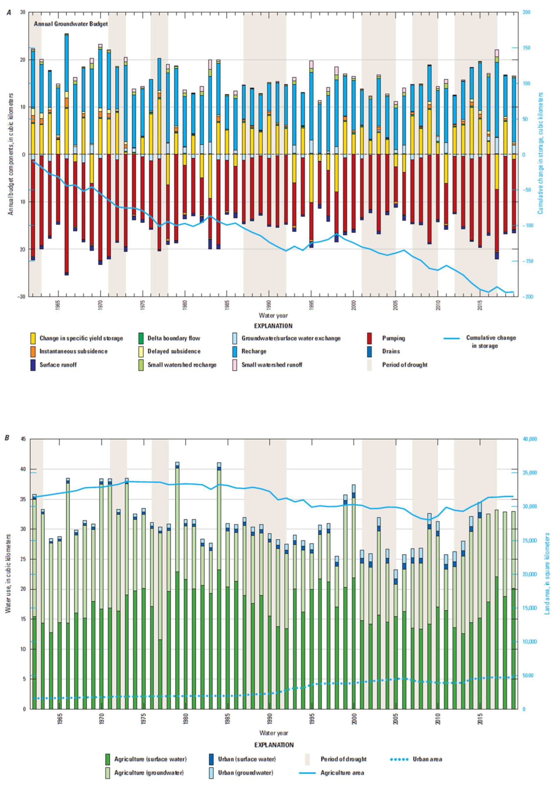
5.1. Hydrologic Budgets

CVHM2 can be used to quantify and synthesize hydrologic budgets for groundwater, surface-water, and water use. The CVHM2 hydrologic budget terms include many complex processes in the integrated surface-water and groundwater system of the Central Valley (Figure 4). CVHM2 simulates the temporal imbalances between water supply and demand, the complex interaction and conjunctive use of surface-water and groundwater, and the resulting land subsidence and changes in groundwater storage. Although SGMA has helped quantify the water-budget components at a local scale, simulated pumping and, ultimately, groundwater storage estimates are still largely determined from the surface-water deliveries and the model-estimated consumptive use of water that calculates supplementary groundwater pumping. With these components, CVHM2 can be used to examine water use and groundwater budgets. For example, as simulated in CVHM2, crop evapotranspiration is about 32 km³ per year, which is relatively large compared to the average annual surface-water inflow to the Central Valley of about 37 km³ per year. This inflow must support agricultural demands and environmental flows, and the distribution of this inflow is not uniform throughout the Central Valley. More than three-quarters of surface-water inflow is in the Sacramento Valley (Figure A5 of [5]), but more than two-thirds of the demand is in the San Joaquin Valley [5]. Land-use data [29] indicate that during droughts, irrigated lands are often fallowed (Figure 4B and Figure S3), and crop evapotranspiration decreases. However, increases in perennial crops have decreased the ability to fallow lands; therefore, the total crop evapotranspiration has become less variable.

CVHM2 can also illustrate temporal changes in water budgets. Surface-water is used when available (generally times with excess precipitation), and groundwater is used when surface-water is not available, either locally or during droughts. As agriculture expanded after the 1960s, irrigation used an average of 29 km³ of water per year from 1962 to 2019 (Figure 4B and Figure S3). Interannual variations in the use of surface-water and groundwater are also subject to climatic variability (Figure 3 and Figure 4). Likewise, the simulated monthly water budgets indicated that precipitation and surface-water deliveries supply most of the water consumed in the early part of the growing season, whereas supply from groundwater pumping increases later in the growing season (Figure 5). In drier years, more groundwater is pumped, and pumping generally starts earlier in the growing season. CVHM2 generally simulates wet years as putting water into groundwater storage and dry years as pulling out of groundwater storage. However, some recharging to the groundwater system almost always occurs during winter or early spring, even during the dry years.

5.1.1. Surface-Water Inflows, Reuse, Diversions, and Water Rights

In CVHM2, the surface-water inflows (average 37 km³ per year) [44] have spatial variability with more inflow from the Sacramento Valley and the Sierra Nevada compared to the San Joaquin Valley and the Coast Ranges, respectively. Diversions into the local irrigation delivery system, which are defined as the amount of flow that is conveyed from a water source, such as a reservoir, stream, or regional canal, average almost half the inflow (17 km³ per year). The amount of water diverted may be different than the actual amount of water used for irrigation. Exploring this distinction between diversion and delivery is important for better understanding simulated water use budgets and the nuances between simulated, reported, and actual water use. Delivery may be less than diversion due to conveyance losses (such as seepage or evaporation). These conveyance losses are not directly simulated in CVHM2 but are indirectly accounted for using irrigation efficiencies. Delivery may also be greater than diversion due to runoff being “reused”. In addition, agriculture water users may not use all the water diverted for irrigation for various reasons, and this water may flow back to the delivery system. The Water Code indicates that if a water right holder fails to beneficially use all or a portion of a water right for a period of five years, “that unused water may revert to the public and shall if reverted, be regarded as unappropriated public water” (California Water Code § 1241). In the San Luis Delta Mendota Water Authority (SLDMWA) area (WBS 10), agricultural water reuse is relatively large compared to other parts of the valley, and CVHM2 was configured to simulate this reuse.

5.1.2. Underflow from Adjacent Watersheds and Surface-Water Flow from Small Ungauged Basins

The amount of water that enters the Central Valley from the surrounding watersheds, which is simulated to enter the model across the eastern and western boundaries, is difficult to estimate accurately. The majority of water entering the Central Valley across eastern and western boundaries is surface-water inflows from reservoir releases (average 37 km³ per year) [44]. To better quantify the magnitude of these smaller inflows that can directly recharge the groundwater system, simulated results from the BCM were used for the boundaries where inflows from streams were not available [56]. BCM simulates 0.55 km³/yr surface inflow from small watersheds that discharges to the stream network and may infiltrate along the streambed and underflow of 0.54 km³/yr, some of which may not reach the Central Valley. Scale factors were used to account for uncertainty in BCM estimates. The scaled BCM mountain-front recharge that flows as groundwater into the Central Valley (referred to here as underflow) from the watersheds surrounding the Central Valley is 0.4 km³/yr for 1962–2019 [47] (Figure 6). There is an additional scaled BCM surface runoff from these small ungauged basins of 0.4 km³/yr, for a total flow of 0.8 km³/yr. CVHM2 uses the BCM estimates and adjusts them during calibration. CVHM2 simulates an average of approximately 12.6 km³/yr of recharge from 1962 to 2019 from all sources, which include the following: (1) net land-surface recharge (precipitation recharge plus agricultural recharge minus the root update of groundwater), (2) small watershed recharge (underflow) and runoff, (3) canal seepage, (4) urban water-use recharge, (5) MAR, and (6) net seepage from streams (Figure 6). About 87% of the total groundwater recharge is from precipitation and agricultural return flow (11.0 km³/yr). The surrounding watersheds supply about 7% of total recharge—about 3% (0.42 km³/yr) of this recharge is from underflow (mountain block recharge) and small watershed runoffs that flow into ephemeral or intermittent streams and then recharge supplies at about 4% (0.45 km³/yr). About 5.5% (0.69 km³/yr) comes from canal seepage, urban water-use recharge, and MAR combined. Net seepage from streams to the groundwater system averages less than 1% of total recharge (0.01 km³/yr). However, net stream seepage varies with water-year type (wet or dry) and was as large as 3.7 km³/yr in 2017 (a wet year) and as small as −2.0 km³/yr in 1968 (a dry year). A negative value indicates that the groundwater system is discharging water to the streams. Other recharge sources include canal seepage, MAR, and urban recharge, and these sources account for the remaining 6% (0.7 km³/yr) of total recharge.

In contrast, recently, 5 km³/yr of subsurface-water flux (often referred to as mountain block recharge) was estimated from the east side of the Central Valley based on the integration of Global Positioning System displacements, Gravity Recovery and Climate Experiment (GRACE) gravity data, reservoir water volumes, and snowpack [61]. The GRACE mission measures changes in the Earth’s gravity field from space using twin-satellite gravimetry data. GRACE data have enabled a continuous and uniform global Terrestrial Water Storage record starting in April 2002 at a spatial resolution OF around 666 km and with monthly sampling [62]. Groundwater storage changes can be quantified from this gravity field [18,19,62,63,64]. These remote regional groundwater storage change estimates are not easily differentiable from small watershed streamflow, soil moisture changes, and evapotranspiration [63,64]. In the recent GRACE study, the subsurface flux (mountain block recharge) was inferred to flow in autumn and winter [52]. Estimates of evapotranspiration from the water-balance model developed from GRACE data [52] were lower compared to estimates of evapotranspiration in the spring and summer; these observed discrepancies likely resulted from estimates of groundwater pumping that were not accounted for [52]. The 5 km³/yr estimate of subsurface-water flux from GRACE data [52] is different from the estimates obtained from c2VSim (1.5 km³/yr), BCM (1.1 km³/yr), and CVHM2 (0.8 km³/yr). c2VSim simulates a small watershed underflow of 1.0 km³/yr to the groundwater system for a slightly different period, 1974–2015. c2VSim simulates a total small watershed flow of approximately 2.5 km³/yr; however, this number includes 1.5 km³/yr surface inflow from small watersheds that discharge to the stream network and may infiltrate along the streambed. Similarly, BCM simulates a total small watershed flow of approximately 1.1 km³/yr; however, this number includes 0.55 km³/yr surface inflow from small watersheds that discharge to the stream network and may infiltrate along the streambed. BCM also does not account for the routing of the flow that might ultimately end in evapotranspiration before the recharge becomes an underflow to the Central Valley, estimated at 0.54 km³/yr. Further, sensitivity analyses of CVHM2 indicate that the magnitude of underflow from adjacent watersheds is small and largely insensitive to parameter changes (parameter sensitivity is shown in the Supplementary Material).

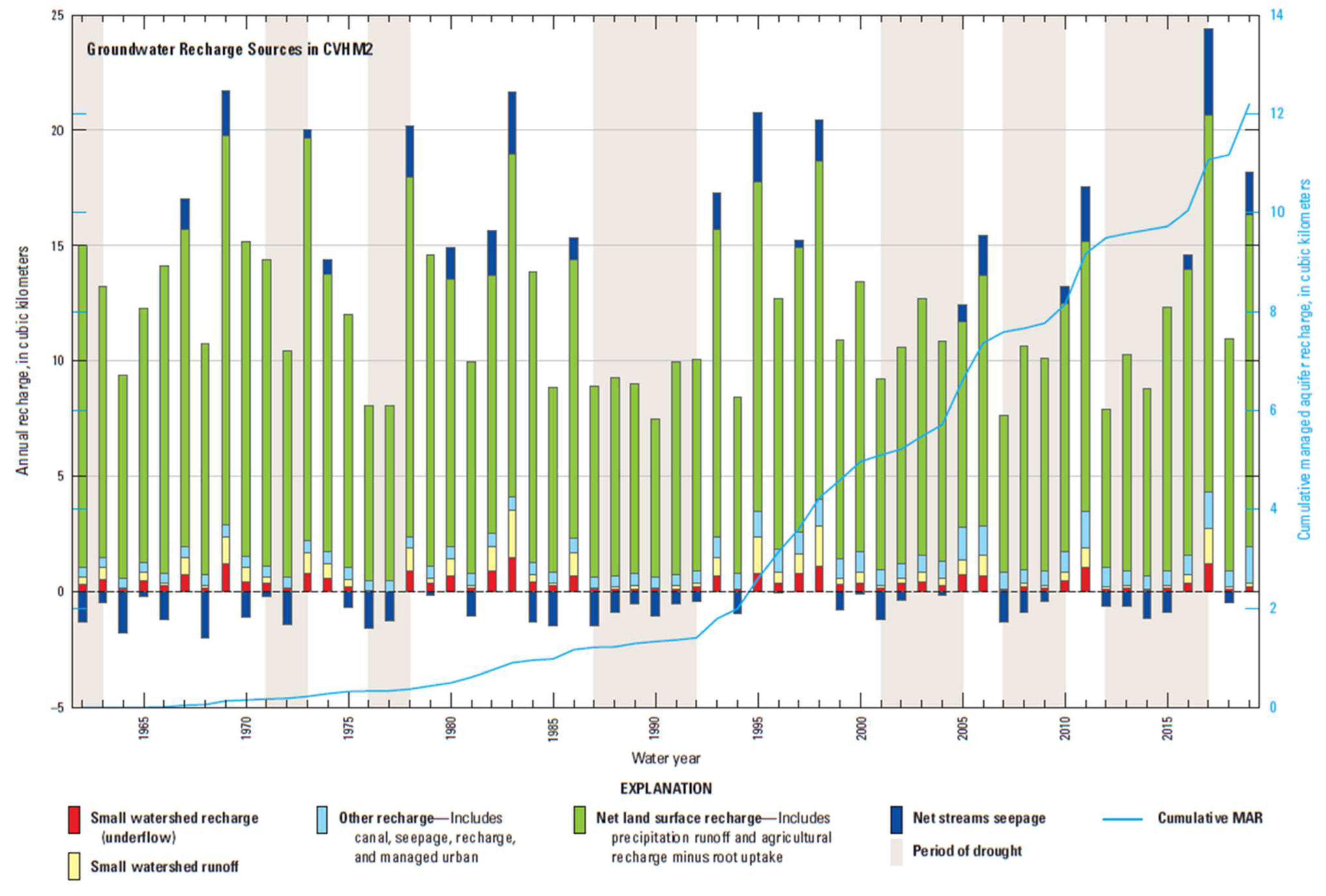
5.1.3. Managed Aquifer Recharge (MAR)

Within the constraints of SGMA and as more pressure is placed on groundwater resources, the demand for groundwater is outweighing the rate of groundwater recharge, and water managers are examining alternative ways to balance the water budget and maintain water supplies [65,66,67,68]. MAR has been used in the Central Valley since the 1960s to help replenish groundwater basins [17,67,68]. MAR is the purposeful recharge of water to aquifers for subsequent recovery or for environmental benefit [65]. Previous studies provide thorough reviews of MAR [67,68]. The five main methods of MAR are as follows: (1) “in lieu” recharge, (2) infiltration ponds, (3) wellfields of storage and recovery wells, (4) seasonal crop flooding, and (5) low-impact development, including permeable pavement, rain gardens, rooftop rainfall capture and recharge, and slow-it–spread-it–sink-it landscaping techniques [65].

In the San Joaquin Valley, decades of groundwater depletion have created an unsaturated aquifer space [14,22] that can be viewed as an opportunity to store water and manage water more effectively. Although aquifers fill more slowly than surface reservoirs, this additional unsaturated aquifer space, which is large compared to the permanently lost aquifer storage space caused by compaction, can be replenished through MAR. Hence, MAR uses aquifer systems as subsurface reservoirs to store surface-water when a surplus is available during wetter periods. This recharged groundwater can then be extracted to meet water demands effectively and economically during droughts, which is a concept often referred to as groundwater banking [69]. The recharged groundwater can also be left in the aquifer to help achieve sustainable groundwater conditions by improving groundwater levels, increasing groundwater storage, reducing land subsidence, diminishing the depletion of interconnected surface-water, improving water quality, and preventing seawater intrusion. In essence, MAR helps provide water supply resiliency by balancing out the seasonal and periodic decreases in surface-water availability.

MAR provides a viable alternative to traditional surface-water reservoirs for storing surplus water. Injection wells and surface impoundments slowly recharge the groundwater system. Surface impoundments are common in the Tulare Basin portion of the Central Valley (Figure 1) and are generally located on alluvial fans or stream channels consisting of sandy sediments, such as the Kern and Kings Rivers. Data were compiled for the major MAR activities in the Central Valley (Figure S2; [43]). MAR operations in the Tulare Basin, including the Kern Water Bank and the Arvin-Edison Water Storage District, each contributed a cumulative storage volume of approximately 2 km³ of water (Figure S2). Recharge and recovery data corresponded with climatic wet and dry periods; that is, more water was spread, and less was recovered during the wet years, and less water was spread, and more was recovered during the dry years. The total cumulative amount of water recharged through MAR facilities was about 12.2 km³ for the years 1962 through 2019 (Figure 6). Even though the magnitude of MAR in an individual year is historically small relative to other recharge amounts in the Central Valley, the cumulative volumes over time can be substantial, especially at the local level. This finding is supported by an analytical approach to assess the impact of MAR operations in the Central Valley [66] suggests that mitigated groundwater droughts and long-term rises in groundwater levels demonstrate the value of long-term MAR operations locally and the contributions of MAR toward sustainable groundwater management. Flood-MAR is any MAR using flood water. In this type of MAR, unused land or a farm or field is flooded by excess surface-water. On-farm recharge, often referred to as Ag-MAR, has become increasingly popular and is often practiced during flood events. In this type of MAR, a farm or field is flooded by surface-water before the growing season. In either Flood-MAR or Ag-MAR, water slowly percolates into the soil, thereby recharging the groundwater system and increasing soil moisture, which can reduce the need for groundwater pumping to meet crop irrigation requirements.

In relation to groundwater budgets and SGMA, MAR is a method of increasing groundwater storage and supply to offset the groundwater storage reductions sustainability indicator. Many of the Central Valley GSAs rely heavily on MAR for groundwater management in their GSPs [2,70]. CVHM2 can be used to quantify the benefits of MAR to the groundwater system at a regional scale. Figure 6 shows the volume of “other recharge” (predominantly MAR—more than 75% of “other recharge” since the early 1990s) relative to land-surface recharge (precipitation and agricultural return flow), underflow from the east- and west-side mountain ranges (small watershed recharge or mountain block and mountain front recharge), recharge from small ungauged streams (small watershed runoff), and seepage from rivers and canals. The expansion of MAR, particularly Flood-MAR, may help mitigate the impacts of climate change due to extreme floods interspersed with longer-term droughts by storing floodwater and pumping this stored water during droughts [39].

As water managers in the Central Valley follow SGMA guidance and adjust for climate change-induced extremes, water-supply availability and the infiltration of MAR will likely become more challenging. Within the aquifer system, there are networks of sand and gravel that provide pathways for recharge. Identifying suitable locations for MAR is complex and involves seeking locations that (1) are geologically favorable (Figure S2), (2) minimize the contamination of fresh groundwater aquifers, (3) are proximal to locations of excess water, and (4) contain compatible land use and conveyance systems to deliver water to recharge areas. Mapping the sand and gravel networks could help identify geologically suitable surface spreading areas so that recharge can be maximized and the interconnected confined aquifer can be repressurized. Data obtained from the California Department of Water Resource’s AEM survey program can help state and local agencies identify sites for groundwater recharge projects that provide the most benefit [35,37]. Other AEM or ground-based transient electromagnetics(TEM) methods could also be used to more accurately resolve the top 50 to 100 m for the assessment of recharge potential [35].

5.1.4. Changes in Groundwater Storage

Two studies incorporating numerical models were used to examine the history of changes in groundwater storage in the Central Valley; the original Regional Aquifer System Analysis (RASA) Central Valley Model has data prior to 1962 and has associated calculations described by [22] and the CVHM2 (Supplementary Material) (Figure 4 and Figure 7). The combined results of these two studies simulate a decline in groundwater levels from the onset of agricultural irrigation development (approximately 1900) until 1977, which resulted in a loss of 74 km³ of storage [20,22]. An additional 85 km³ of storage loss is simulated in CVHM2 from 1978 to 2019 (Supplementary Material). This depletion of storage is made up of the following three components: (1) water-table release; (2) inelastic compaction release; and (3) elastic release [22]. The water-table release is water from storage as a result of dewatering shallow aquifers and lowering the groundwater table (49 km³ from 1900 to 1977 and 73 km³ from 1978 to 2019). Inelastic compaction is irreversible and occurs when applied stress exceeds pre-consolidation stress so that the pores of the sediments are rearranged, and pore volume is permanently reduced (21 km³ from 1900 to 1977 [22,71] and 12 km³ from 1978 to 2019). The loss of storage from inelastic compaction causes a permanent loss of pore space that, in turn, is balanced by an equivalent volume of land subsidence [22]. The reversible elastic release is water from storage as a result of the expansion of the compressed water and sediments when the hydraulic pressure is reduced—3.7 km³ from 1900 to 1977 and −0.1 km³ from 1978 to 2019 (negative value indicates a net gain in elastic storage) [22].

The results from CVHM2 were analyzed to quantify and understand long-term groundwater storage and depletion trends for the period 1962–2019. During this period, groundwater withdrawn from storage averaged 3.1 km³ per year, representing about 22% of annual pumping (14.4 km³) (Figure 4). The rest of the groundwater pumping comes from recharge sources (Figure 6). Nevertheless, the lowering of groundwater levels in the upper and lower zones caused an increase in pumping head lifts and pumping costs, changes in water quality, and land subsidence [5,22]. After surface-water delivery systems were put in place, groundwater pumping decreased, and groundwater levels rose in many areas [5,22]. From 2000 to 2019, there was an increase in pumping in dry years and an average storage loss of about 3.5 km³ per year (Figure 6 and Figure 7). The periods of more storage loss and increased pumping generally occurred during droughts or following changes in land use. The most rapid groundwater storage losses occurred during the droughts of 2007–2009 (24 km³ of loss over 3 years) and 2012–2016 (37 km³ of loss over 5 years) (Figure 4 and Figure 7). As [19] also found, reduced net inflows, the transition from row to tree crops, and higher evapotranspiration led to most of the groundwater loss in the 2012–2016 drought. Much of the 2012–2016 groundwater loss was from the San Joaquin Valley, with approximately one-third from the San Joaquin Basin and two-thirds from the Tulare Basin (Figure 7). The decline during the 2012–2016 drought period was more widespread and higher in magnitude compared to the declines in the 2007–2009 period.

CVHM2 also simulates the monthly and annual variability in groundwater storage due to climate variability. The results demonstrated that during the wet years, groundwater storage typically increased, whereas in dry years, groundwater storage decreased (Figure 7). Annual climate effects on groundwater storage were most notable during the droughts of 2007–2009 and 2012–2016, and the changes in groundwater levels between these drought periods simulated in CVHM2 were analyzed to better understand the location of groundwater storage depletion during these drought periods. Figure 8A shows that most groundwater depletion during the 2007–2009 drought period occurred in the southern part of the Central Valley (Tulare Basin), and the most extreme changes took place in the northwestern part of the Tulare Basin. Simulated groundwater level declines of up to 10 m were observed in some areas of the eastern and northeastern San Joaquin Valley. Figure 8B shows that groundwater-level declines occurred in the same portions of the Tulare Basin and eastern San Joaquin Valley during the 2012–2016 drought period. However, during the 2012–2016 drought period, groundwater-level declines were observed in a portion of the western San Joaquin Valley that did not have observed groundwater-level declines during the 2007–2009 drought period. The groundwater level decline in the northern San Joaquin Valley was also more widespread during the 2012–2016 drought period compared to the 2007–2009 drought period, with declines of up to 10 m occurring in parts of the east side of the San Joaquin Valley. In addition, groundwater levels declined in parts of the Sacramento Valley. The southernmost part of the San Joaquin Valley was simulated to show increased groundwater levels near MAR facilities.

Famiglietti et al. [18] identified the need for quantifying groundwater storage changes at frequent temporal samplings to improve the management of groundwater resources and characterization of groundwater depletion. In the Central Valley, GRACE data were used to compute groundwater depletion during 2002–2011. One GRACE-based study estimated the depletion trend during the drought from January 2006 to July 2009 to be 41 km³ [39]. A later GRACE-based study estimated that about 55 km³ of groundwater was lost from the Central Valley during the 2007–2009 and 2012–2016 droughts combined [19]. CVHM2 simulated 24 km³ of depletion over a similar period to the first study (from the start of WY 2007 to the end of WY 2009). With the 2007–2009 and 2012–2016 droughts combined, CVHM2 simulated 62 km³ of depletion. The GRACE estimates and the CVHM2 storage change estimates were similar in magnitude and areal extent [19,39,72]. These numbers were also similar to the simulated total volume of 30 km³, which was the estimated loss through a separate method using only Global Positioning System deformation data [72]. GRACE-derived estimates of Central Valley groundwater loss were similar during droughts but not between droughts.

The scale of these storage change estimates is regional in nature. Due to the limited spatial resolution and the associated errors in disaggregating GRACE-derived total water storage [39], the application of GRACE data is not feasible at the local scale [63]. The resolution, soil moisture accuracy, and computational methods have limitations even at the scale of the Central Valley. Although a more detailed scale than GRACE-derived estimates, the CVHM2 encompasses a larger scope for use by managers who need modeling information at regional to subregional scales. However, more detailed models and analyses are required for the finer-resolution water budgets needed by local water managers aiming to meet the guidelines established by the SGMA.

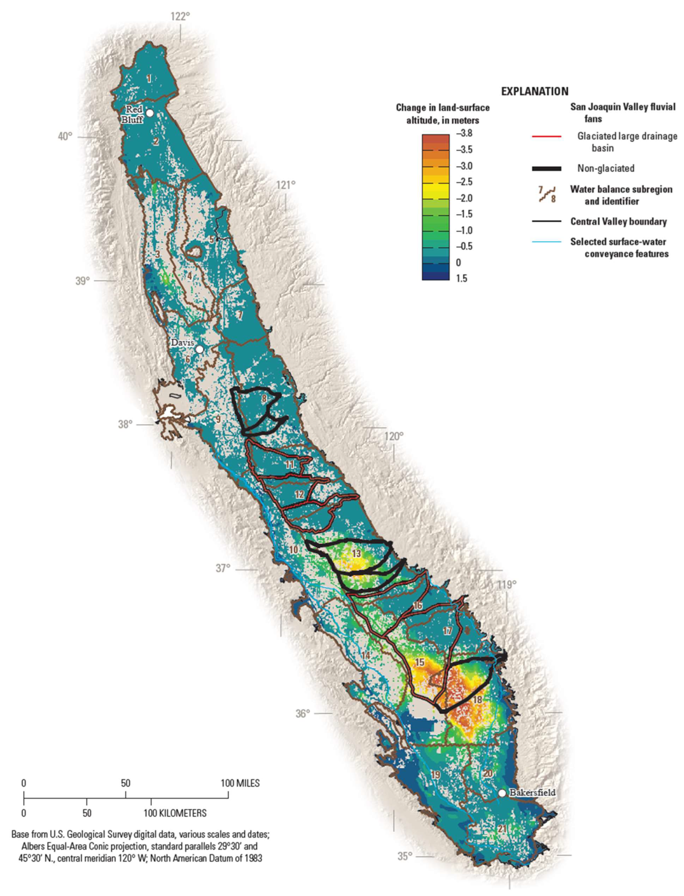
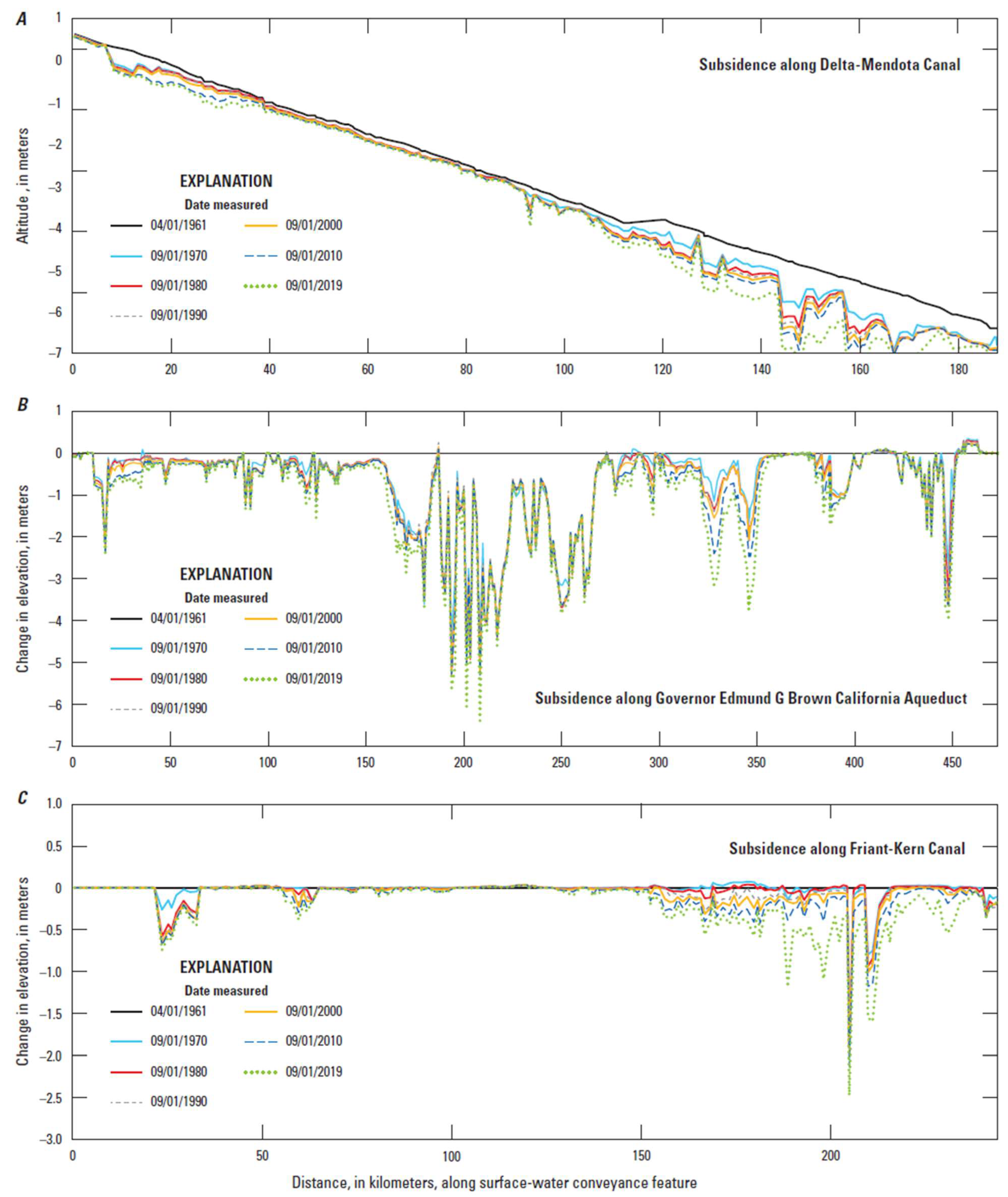
5.2. Land Subsidence

Land subsidence affects many of the world’s major aquifers [73,74,75]. The largest volume of land subsidence in the world caused by human activities is in the Central Valley [20,58]. In the Central Valley, land subsidence is typically caused by groundwater extraction that results in a one-time release of water from compacting, fine-grained deposits [21]. Once the effective stress increases beyond a pre-consolidation stress level, inelastic deformation causes a permanent loss in the aquifer-system pore space that results in irreversible land subsidence [71,76,77,78]. Groundwater storage loss can be delayed, instantaneous, or a combination of both. The location, thickness, and distribution of the finer-grained deposits When combined with the location and magnitude of groundwater extraction, the locations, thicknesses, and distributions of the finer-grained deposits are directly related to the extent, magnitude, and timing of land subsidence. Approximately 70% of the thickness of the Central Valley aquifer system is composed of fine-grained sediments [5,14,34] (Figure 2) that are susceptible to aquifer-system compaction when the sediments are depressurized by groundwater pumping. Historically, compaction and subsidence rates have been measured by a variety of methods, including benchmark surveys, extensometers [79], continuous Global Positioning System (cGPS), an interferometric synthetic aperture radar (InSAR), and uninhabited aerial vehicle synthetic aperture radar (UAVSAR) (Figure 9; [46] and Supplementary Material). Recently, these methods have been combined with GRACE measurements to characterize groundwater storage dynamics and their uses and limitations [14,58,61,80]. Recent land subsidence rates have been compiled and mapped using satellite data (Figure 9 and Figure 10) [81].

Extensive groundwater pumping through much of the early-to-mid-1900s resulted in groundwater declines and land subsidence throughout much of the San Joaquin Valley [2,5,22,40]. The importation of surface-water to this area via the Delta–Mendota Canal began in the 1950s [5,6]. The Governor Edmund G Brown California Aqueduct began importing surface-water to this area in the 1970s, and the accompanying reduction in groundwater pumping caused groundwater levels to rise and land subsidence to virtually cease (Figure 3) [2,5,22,40]. During the 1970s, 80s, and 90s, there was very little land subsidence, except during the 1976–1977 drought, when pumping from wells sharply increased due to the lack of surface-water supplies [5,6,38] (Figure 4). This increased pumping caused groundwater levels to drop below their previous lows. Stored water was released due to inelastic compaction, and land subsidence resumed (Figure 3 and Figure 4). By the early 1980s, more than one-half of the San Joaquin Valley, or about 13,500 km², had undergone land subsidence of more than 0.3 m [22]. As of 1983, land subsidence in the San Joaquin Valley had either slowed considerably or ceased ([84]; Figure 3 and Figure 4; Supplementary Material). Land use changes, water restrictions, and recurring droughts resulted in substantial observed and simulated land subsidence in 2007–2009 and 2012–2016, but recent occurrences were observed at additional locations that were different from previous historical locations (Figure 10; [14]).

Despite the long history of studying and monitoring land subsidence, the key hydrogeological factors influencing the spatial variation in land subsidence are typically not well mapped [40]. In the Central Valley, land subsidence occurs primarily in areas where there are numerous clay layers interlayered with sand and gravel [14,40,58,74]. To help explain the variability in location and magnitude of land subsidence, simulated land subsidence was compared with local geological information and groundwater-level measurements retrieved from USGS [85] and the California Department of Water Resources [86] databases (Figure 10). Satellite data and simulated land subsidence from CVHM2 were used to further evaluate the spatial extent and magnitude of land subsidence during the period WY 1962–2019 (Figure 4 and Figure 10). As mentioned previously, the magnitude and rate of land subsidence varies depending on the hydraulic and mechanical properties and consolidation history of the aquifer system. As was performed by [14,40], the extent of land subsidence was compared with the extent of alluvial fans from the Sierra Nevada ([83]; Figure 2 and Figure 10). In general, deposits sourced from the Coast Ranges and the non-glaciated alluvial fan deposits sourced from the Sierra Nevada are finer-grained and as a result more compressible, resulting in greater land subsidence. Conversely, the upper reaches of the large-drainage area glaciated alluvial fans that are relatively coarser-grained had much lower rates of land subsidence. These are general broad brushed correlations; a more detailed examination of the driller’s logs, groundwater levels, and the mapping of the aquifer system, such as with AEM, could help assess the vulnerability of local areas to land subsidence. In addition, accurate conceptual models could guide the sitting of expensive monitoring wells for groundwater levels and compaction.

The loss of groundwater storage to inelastic compaction resulted in land subsidence being one of six issues that GSAs are intended to address [15]. In the San Joaquin Valley, elastic (reversible) compaction recovers rapidly on an annual basis (Figure 11), but inelastic (permanent) compaction has resulted in land subsidence and has damaged infrastructure [21,74,80]. Land subsidence has damaged some critical water conveyance systems, including the Delta–Mendota Canal, the Friant-Kern Canal (60% of capacity lost in some stretches), and the Governor Edmund G Brown California Aqueduct (more than 20% of capacity lost) [87] (Figure 10). Bridges over these and other canals impede flow, and some dams on water courses have sunk to the extent that they no longer create storage capacity [2]. Land subsidence also permanently reduces the capacity of aquifer systems to store water. Between 1962 and 2019, approximately 27 km³ of storage loss was attributed to inelastic compaction.

GSAs vary widely in their approaches to addressing land subsidence, but most GSPs include thresholds for groundwater levels, land subsidence, or both [2]. In several areas where infrastructure has already been damaged, agencies are setting thresholds to avoid additional land subsidence [15,27,87]. The portion of the Central Valley affected by land subsidence due to groundwater extraction includes much of the southern part of the San Joaquin Valley and smaller areas in the Sacramento Valley (Figure 10). In southern and western portions of the San Joaquin Valley, between 1925 and 1977, the land near Mendota sank by nearly 9 m, and the majority of compaction occurred below the Corcoran Clay [79,88]. During 1925–2019, like CVHM and C2VSim, CVHM2 simulated most of the pumping and subsidence in this region from the deeper confined portion of the aquifer below this clay-confining unit. Groundwater-level changes more rapidly in confined systems, and reductions in pressure result in subsidence. The pressurized nature of this part of the aquifer system intensifies the rate of compaction of the fine-grained materials in the Central Valley. The largest amount of land subsidence recorded that was attributed to groundwater withdrawals in the Central Valley is in the finer-grained areas below the Corcoran Clay and in the relatively fine-grained area near the town of Pixley in western WBS 18 (Figure 10). Figure 11 shows that the groundwater levels near Mendota are declining at a much faster rate in the deeper part of the system. Compaction and land subsidence track these groundwater-level change differences, with most of the compaction occurring in the deeper confined system. The land surface is sinking at a much faster rate than the sediments are compacting in an anchored extensometer that records compaction in the shallow part of the system.

CVHM2 simulates the magnitudes of each of the components of the groundwater storage change (Figure 12A). These storage components are unconfined storage (specific yield storage), instantaneous elastic storage, instantaneous inelastic storage, delayed elastic storage, and delayed inelastic storage. From 1962 to 2019, 86% of the storage loss was from unconfined storage loss (178 km³), 7% of the storage loss was from delayed inelastic storage loss (14 km³), and 7% of storage loss was from instantaneous inelastic storage loss (13 km³). The storage loss from elastic storage loss was small (less than 0.3%). The instantaneous and delayed (slower drainage from thicker clay beds) storage losses were similar in overall magnitude from 1962 to 2019, but the storage losses varied greatly in location and timing. Water managers can use this information to manage water more effectively and reduce storage loss and land subsidence in the Central Valley.

CVHM2 simulates the magnitude of the change in storage from the shallow and deep aquifer systems and the Corcoran Clay (Figure 12B), which has previously been difficult to quantify. Most of the storage loss was from the shallow unconfined to semi-confined portion of the aquifer system (layers 1–5, generally <100 m) located above the Corcoran Clay (where present). A small amount of storage was lost in the Corcoran Clay (Layers 6–8). About 20% of the storage loss occurred in the deeper confined portions of the aquifer system (Layers 9–13) located below the Corcoran Clay.

Figure 13A–C shows the simulated cumulative land subsidence for each decade along the Delta–Mendota Canal, Governor Edmund G Brown California Aqueduct, and the Friant-Kern Canal. Simulated land subsidence along the Delta–Mendota Canal (Figure 13A) is largest at the bottom of the canal from approximately km 113 (mile 70) to the end of the canal (km 245 (mile 152)). Much of the simulated land subsidence took place from 1960 to 1970 and from 2000 to 2019. The magnitude and rate of land subsidence along the Governor Edmund G Brown California Aqueduct (Figure 13B) vary. The largest magnitude of land subsidence occurred from approximately km 161 (mile 100) to km 241 (mile 150), and most of this subsidence occurred during 1960–1970.

Another area of land subsidence along the Governor Edmund G Brown California Aqueduct is from approximately km 322 (mile 200) to km 354 (mile 220). In this area, as much as 2 m of land subsidence occurred during 1960–1970, and then land subsidence virtually stopped with the importation of surface-water starting in the 1970s [2,5,22,40]; however, land subsidence started reoccurring in the 2000s, and about 1 m more of subsidence occurred during 2000–2019. Land subsidence along the Friant-Kern Canal (Figure 13C) is mostly located from about km 145 (mile 90) to the end of the canal (195.5 km (mile 121.5)). This length corresponds to the 53 km stretch of the canal where the Friant-Kern Canal Middle Reach Capacity Correction Project is taking place to restore flow capacity in the canal [89]. The rate of land subsidence has not decreased near the Friant-Kern Canal (Figure 10, Figure 11 and Figure 13) following the enactment of SGMA in 2014 [15].

Monitoring and simulating land subsidence can provide insight into the management of groundwater for meeting the management constraints defined by the SGMA. CVHM2 was developed to account for the time-dependent deformation in the subsurface from which groundwater is being pumped [14,36]. Groundwater levels within fine-grained clay interbed and aquifers continue to equilibrate beyond the drought period and vary spatially. As a result, the residual compaction of the fine-grained materials and land subsidence continues. The rate of equilibration of these groundwater levels, and ultimately the rate and extent of subsidence, depends on the vertical conductivity between the coarse-grained portion of the aquifer (which does not compact residually) and the interbeds, with head differences between the coarse-grained portion of the aquifer and the interbeds, and the thickness of the fine-grained interbeds. An equilibration period of 0.5–1.5 years was simulated for the CVHM2-modeled area; however, the equilibration period varied widely within the San Joaquin Valley. Corcoran Clay is believed to have a significantly lower vertical hydraulic conductivity [5,14,22] than the surrounding materials and likely will drain for more than a thousand years (Supplementary Material).

Simulated land subsidence in the San Joaquin Valley from 1962 to 2009 (Figure 14A) shows a large amount of land subsidence in the San Joaquin Valley. Figure 14B shows that from 2000 to 2019, land subsidence occurred in many of the same areas of the San Joaquin Valley but was more localized and occurred at lower rates. Exceptions to this pattern are that land subsidence in the southwestern San Joaquin Valley and southernmost San Joaquin Valley has mostly ceased. From 2012 to 2016 (Figure 14C), the location of subsidence is similar to 2000 to 2019, with total land subsidence in just these five years being roughly half of the total land subsidence over the last 20 years (Figure 14B). Much of the subsidence occurring in just this 5-year period is likely due to drought and recent land use changes.

6. Conclusions

Water scarcity, particularly the decrease in groundwater availability, is a global problem and is particularly problematic in California’s Central Valley. Climate variability, including droughts of increasing frequency and intensity and the overuse has led to increasing concerns related to water sustainability [60]. Groundwater overuse has severely impacted SGMA groundwater basins in the Central Valley and has led to falling groundwater levels, the permanent loss of groundwater and storage capacity, and land subsidence.

Options available to support groundwater sustainability include augmenting water supplies, reducing water demand, or some combination of the two. Integrated hydrologic modeling is critical to understanding the dynamics of the management strategies. On a regional scale, the CVHM2 shows changes in groundwater level, storage, and land subsidence and the relationships of these changes to land use, climate, and management strategies. Combined with historical approximations, CVHM2 estimates that approximately 158 km³ of groundwater storage has been lost in the Central Valley over the last 120 years. About 15% of this depletion is estimated to be irreversible and accounts for most of the observed land subsidence in the modeled area. This long-term decrease in storage is large but only represents about 15% of the more than 990 km³ of freshwater estimated by [22] to be stored in the upper 300 m of sediments in the Central Valley (Figure 5 and Figure 7). Based on these estimates, the upper 300 m of groundwater basins store about a 20-year supply of water for use based on consumption estimates from CVHM2. For comparison, the total surface-water storage capacity in California is 52 km³—or a one-year supply for farms, cities, and the environment [12]. Typically, groundwater supplies about one-third of the water for cities and farms, and during severe droughts, groundwater provides more than half of the water used [12]. From 1962 to 2019, the Central Valley lost about 27 km³ of water due to inelastic compaction, or about 3% of the estimated pumping of 835 km³ for the entire Central Valley. Most of the water released from inelastic compaction occurred in the Tulare Basin (Figure 4 and Figure 10). For the entire Central Valley, the amount of water released from unconfined storage in the aquifer was 155 km³ or about 19% of the estimated pumping for 1962–2019 (Figure 4 and Figure 7).

Overdraft is a major issue in the San Joaquin Valley; however, the CVHM2 shows that climate variability and more recent changes in land use are affecting the water budget and subsidence and will likely be considered in future decisions regarding water management. Resource managers and stakeholders can use CVHM2 and our study results to better understand the drivers of water budgets and plan for continued land subsidence in the Central Valley. CVHM2 includes ancillary datasets used to construct model input and can be used to assess regional changes in groundwater availability and land subsidence and inform decisions related to conjunctive water resource management. It provides hydrologic data and can be used to assist decision makers in conjunctive water resource management. Specifically, CVHM2 can be used to guide and provide datasets to GSAs and allow for comparisons of GSAs.

CVHM2 could also be used in conjunction with local models and other tools such as C2VSim, various forms of gravity, or AEM. As the SGMA continues to be implemented through the six interconnected sustainability indicators, water managers will likely need to identify the limiting factors specific to their local areas, including the spatial and temporal balancing of supply and demand, including variable usage and climate fluctuations. CVHM2 provides an integrated platform and data compilation to assess these indicators.

The ability to maximize groundwater storage can help water managers maintain sustainable water supplies throughout varying conditions caused by climate extremes. The mapping of aquifer-system characteristics could help rewater managers identify geologically suitable surface spreading areas so that recharge can be maximized. Data obtained from AEM survey programs can be used to map the large-scale texture of aquifer systems and help water managers determine the best areas to recharge the aquifer system.

The amount and rate of land subsidence is controlled by groundwater head dynamics and geologic conditions encompassing a complex combination of fast- and slow-draining clay beds and interbeds. In some locations, the magnitude of land subsidence varies within short distances (horizontally and vertically). Finer-grained sediments are generally more compressible than coarser-grained deposits regardless of their source, resulting in greater land subsidence under equivalent applied stresses, such as declining groundwater levels. As a result, the upper reaches of the large-drainage area glaciated alluvial fans are relatively coarser-grained and have much lower rates of land subsidence. The valley deposits sourced from the Coast Ranges and the non-glaciated alluvial fan deposits sourced from the Sierra Nevada have substantially higher rates of land subsidence. These broadly measured and simulated correlations can be used by water managers to optimize locations for groundwater pumping and surface-water deliveries. More refined local-scale assessments of the vulnerability of local areas to land subsidence and the detailed mapping of the aquifer system could be completed with local drilling, mapping, and AEM. Much of the Tulare Basin has had delay and non-delay compaction at various times, resulting in land subsidence. When groundwater levels reach historically low levels, delay and non-delay compaction occur. Conversely, groundwater levels in the eastern San Joaquin Basin (WBS 13; Figure 1) have been declining steadily since the 1960s, and most of the land subsidence is related to non-delay (or instantaneous) compaction. As groundwater levels are declining in the shallow parts of the system (which are often semi-confined due to their high clay content), even the shallow parts of the aquifer system are measured and simulated as compacting and contributing to land subsidence. CVHM2 can be used by water managers to simulate these complex and interrelated conditions for decision support purposes, particularly for decisions related to subsidence. Various scenarios related to climate or land-use changes can be readily used to address and analyze the impacts of subsidence on infrastructure.

References

1. Turner, S.W.D.; Hejazi, M.; Calvin, K.; Kyle, P.; Kim, S. A Pathway of Global Food Supply Adaptation in a World with Increasingly Constrained Groundwater. Sci. Total Environ. 2019, 673, 165–176. [Google Scholar] [CrossRef] [PubMed]
2. California Department of Water Resources. California’s Groundwater Update 2020 (Bulletin 118); California Department of Water Resources: Sacramento, CA, USA, 2020. [Google Scholar]
3. De Graaf, I.E.M.; Sutanudjaja, E.H.; Van Beek, L.P.H.; Bierkens, M.F.P. A High-Resolution Global-Scale Groundwater Model. Hydrol. Earth Syst. Sci. 2015, 19, 823–837. [Google Scholar] [CrossRef]
4. Bierkens, M.F.P.; Wada, Y. Non-Renewable Groundwater Use and Groundwater Depletion: A Review. Environ. Res. Lett. 2019, 14, 063002. [Google Scholar] [CrossRef]
5. Faunt, C.C. (Ed.) Groundwater Availability of the Central Valley Aquifer, California; U.S. Geological Survey Professional Paper 1766; U.S. Geological Survey: Reston, VA, USA, 2009; ISBN 978-1-4113-2515-9.
6. California Department of Water Resources. The California Water System. Available online: https://water.ca.gov/Water-Basics/The-California-Water-System (accessed on 24 November 2023).
7. Dettinger, M.D.; Cayan, D.R.; Meyer, M.K.; Jeton, A.E. Simulated Hydrologic Responses to Climate Variations and Change in the Merced, Carson, and American River Basins, Sierra Nevada, California, 1900–2099. Clim. Chang. 2004, 62, 283–317. [Google Scholar] [CrossRef]
8. Kattelmann, R. Very Warm Storms and Sierra Nevada Snowpacks. In Proceedings of the 65th Annual Western Snow Conference, Banff, AB, Canada, 4–8 May 1997; pp. 125–129. [Google Scholar]
9. Cayan, D.; Tyree, M.; Dettinger, M.; Hidalgo, H.; Das, T.; Maurer, E.; Bromirski, P.D.; Flick, R.E. Climate Change Scenarios and Sea Level Rise Estimates for the California 2009 Climate Change Scenarios Assessment; Oceanography Program, California Department of Parks & Recreation; UC San Diego: San Diego, CA, USA, 2009. [Google Scholar]
10. Dettinger, M.D.; Ralph, F.M.; Das, T.; Neiman, P.J.; Cayan, D.R. Atmospheric Rivers, Floods and the Water Resources of California. Water 2011, 3, 445–478. [Google Scholar] [CrossRef]
11. United States Census Bureau. United States Census Bureau California Statistis. Available online: https://data.census.gov/profile/California (accessed on 1 April 2024).
12. Hanak, E.; Lund, J.R.; Mount, J.; Gurdak, J.; Harter, T.; Viers, J.; Escriva-Bou, A.; Fisher, A.T.; Fogg, G.; Gray, B. California’s Water: Storing Water; Public Policy Institute of California: San Francisco, CA, USA, 2018; p. 4. [Google Scholar]
13. Dettinger, M.D.; Anderson, M.L. Storage in California’s Reservoirs and Snowpack in This Time of Drought. San Fr. Estuary Watershed Sci. 2015, 13, 1. [Google Scholar] [CrossRef]
14. Faunt, C.C.; Sneed, M.; Traum, J.; Brandt, J.T. Water Availability and Land Subsidence in the Central Valley, California, USA. Hydrogeol. J. 2016, 24, 675–684. [Google Scholar] [CrossRef]
15. California Department of Water Resources. Sustainable Groundwater Management Act (SGMA). Available online: https://water.ca.gov/Programs/Groundwater-Management/SGMA-Groundwater-Management (accessed on 24 November 2023).
16. California Department of Water Resources. Basin Prioritization. Available online: https://water.ca.gov/Programs/Groundwater-Management/Basin-Prioritization (accessed on 24 November 2023).
17. Scanlon, B.R.; Keese, K.E.; Flint, A.L.; Flint, L.E.; Gaye, C.B.; Edmunds, W.M.; Simmers, I. Global Synthesis of Groundwater Recharge in Semiarid and Arid Regions. Hydrol. Process. 2006, 20, 3335–3370. [Google Scholar] [CrossRef]
18. Famiglietti, J.S.; Lo, M.; Ho, S.L.; Bethune, J.; Anderson, K.J.; Syed, T.H.; Swenson, S.C.; de Linage, C.R.; Rodell, M. Satellites Measure Recent Rates of Groundwater Depletion in California’s Central Valley. Geophys. Res. Lett. 2011, 38, L03403. [Google Scholar] [CrossRef]
19. Xiao, M.; Koppa, A.; Mekonnen, Z.; Pagán, B.R.; Zhan, S.; Cao, Q.; Aierken, A.; Lee, H.; Lettenmaier, D.P. How Much Groundwater Did California’s Central Valley Lose during the 2012–2016 Drought? Geophys. Res. Lett. 2017, 44, 4872–4879. [Google Scholar] [CrossRef]
20. Bertoldi, G.L.; Johnston, R.H.; Evenson, K.D. Ground Water in the Central Valley, California: A Summary Report; Professional Paper; U.S. Geological Survey: Reston, VA, USA, 1991; p. 56.
21. Galloway, D.L.; Jones, D.R.; Ingebritsen, S.E. Land Subsidence in the United States; Circular; U.S. Geological Survey: Reston, VA, USA, 1999; p. 177.
22. Williamson, A.K.; Prudic, D.E.; Swain, L.A. Ground-Water Flow in the Central Valley, California; Professional Paper; U.S. Geological Survey: Reston, VA, USA, 1989; p. 127.
23. Gailey, R.M. Inactive Supply Wells as Conduits for Flow and Contaminant Migration: Conditions of Occurrence and Suggestions for Management. Hydrogeol. J. 2017, 25, 2163–2183. [Google Scholar] [CrossRef]
24. Levy, Z.F.; Jurgens, B.C.; Burow, K.R.; Voss, S.A.; Faulkner, K.E.; Arroyo-Lopez, J.A.; Fram, M.S. Critical Aquifer Overdraft Accelerates Degradation of Groundwater Quality in California’s Central Valley During Drought. Geophys. Res. Lett. 2021, 48, 10. [Google Scholar] [CrossRef]
25. Duffy, W.G.; Kahara, S.N. Wetland Ecosystem Services in California’s Central Valley and Implications for the Wetland Reserve Program. Ecol. Appl. 2011, 21, S128–S134. [Google Scholar] [CrossRef]
26. Gailey, R.M.; Lund, J.R.; Medellín-Azuara, J. Domestic Well Reliability: Evaluating Supply Interruptions from Groundwater Overdraft, Estimating Costs and Managing Economic Externalities. Hydrogeol. J. 2019, 27, 1159–1182. [Google Scholar] [CrossRef]
27. Hanak, E.; Lund, J.; Arnold, B.; Escriva-Bou, A.; Gray, B.; Green, S.; Harter, T.; Howitt, R.; MacEwan, D.; Medellín-Azuara, J. Water Stress and a Changing San Joaquin Valley; Public Policy Institute of California: San Francisco, CA, USA, 2017; p. 48. [Google Scholar]
28. Hanak, E.; Escriva-Bou, A.; Gray, B.; Green, S.; Harter, T.; Jezdimirovic, J.; Lund, J.; Medellín-Azuara, J.; Moyle, P.; Seavy, N. Water and the Future of the San Joaquin Valley; Public Policy Institute of California: San Francisco, CA, USA, 2019; p. 15. [Google Scholar]
29. Seymour, W.A.; Faunt, C.C. Central Valley Hydrologic Model Version 2 (CVHM2): Land Use Properties (Ver. 3.0, October 2023); U.S. Geological Survey Data Release; U.S. Geological Survey: Reston, VA, USA, 2022. [CrossRef]
30. Mall, N.K.; Herman, J.D. Water Shortage Risks from Perennial Crop Expansion in California’s Central Valley. Environ. Res. Lett. 2019, 14, 9. [Google Scholar] [CrossRef]
31. California Department of Water Resources Land IQ California 2014. Available online: https://catalog.data.gov/dataset/i15-crop-mapping-2014-dec52 (accessed on 15 April 2024).
32. Brush, C.F.; Belitz, K.; Phillips, S.P. Estimation of a Water Budget for 1972–2000 for the Grasslands Area, Central Part of the Western San Joaquin Valley, California; Scientific Investigations Report; U.S. Geological Survey: Reston, VA, USA, 2004; p. 59.
33. Marcelli, M.F.; Shepherd, M.M.; Faunt, C.C. Central Valley Hydrologic Model Version 2 (CVHM2): Well Log Lithology Database and Texture Model; U.S. Geological Survey Data Release; U.S. Geological Survey: Reston, VA, USA, 2022. [CrossRef]
34. Faunt, C.C.; Belitz, K.; Hanson, R.T. Development of a Three-Dimensional Model of Sedimentary Texture in Valley-Fill Deposits of Central Valley, California, USA. Hydrogeol. J. 2010, 18, 625–649. [Google Scholar] [CrossRef]
35. Knight, R.; Smith, R.; Asch, T.; Abraham, J.; Cannia, J.; Viezzoli, A.; Fogg, G. Mapping Aquifer Systems with Airborne Electromagnetics in the Central Valley of California. Groundwater 2018, 56, 893–908. [Google Scholar] [CrossRef] [PubMed]
36. Smith, R.; Knight, R. Modeling Land Subsidence Using InSAR and Airborne Electromagnetic Data. Water Resour. Res. 2019, 55, 2801–2819. [Google Scholar] [CrossRef]
37. California Department of Water Resources. Airborne Electromagnetic (AEM) Surveys. Available online: https://water.ca.gov/Programs/SGMA/AEM (accessed on 25 November 2023).
38. Brush, C.F.; Dogrul, E.C.; Kadir, T.N. Development and Calibration of the California Central Valley Groundwater-Surface Water Simulation Model (C2VSim), version 3.02-CG; Technical Memorandum; California Department of Water Resources: Sacramento, CA, USA, 2013.
39. Scanlon, B.R.; Faunt, C.C.; Longuevergne, L.; Reedy, R.C.; Alley, W.M.; McGuire, V.L.; McMahon, P.B. Groundwater Depletion and Sustainability of Irrigation in the US High Plains and Central Valley. Proc. Natl. Acad. Sci. USA 2012, 109, 9320–9325. [Google Scholar] [CrossRef]
40. Faunt, C.C.; Sneed, M. Water Availability and Subsidence in California’s Central Valley. San Fr. Estuary Watershed Sci. 2015, 13, 4. [Google Scholar] [CrossRef]
41. California Department of Water Resources. C2VSimCG, version 1.0; California Department of Water Resources: Sacramento, CA, USA, 2022.
42. California Department of Water Resources. C2VSimFG, version 1.01; California Department of Water Resources: Sacramento, CA, USA, 2023.
43. Bond, S.; Jachens, E.R.; Faunt, C.C. Central Valley Hydrologic Model Version 2 (CVHM2): Water Banking for Water Years 1961–2019 (Ver. 2.0, Aug 2023); U.S. Geological Survey Data Release; U.S. Geological Survey: Reston, VA, USA, 2022. [CrossRef]
44. Earll, M.M. Central Valley Hydrologic Model Version 2 (CVHM2): Surface Water Network for Water Years 1922–2019; U.S. Geological Survey Data Release; U.S. Geological Survey: Reston, VA, USA, 2022. [CrossRef]
45. Faunt, C.C. Central Valley Hydrologic Model Version 2 (CVHM2): Model Setup Files; U.S. Geological Survey Data Release; U.S. Geological Survey: Reston, VA, USA, 2022. [CrossRef]
46. Faunt, C.C.; Stamos-Pfeiffer, C.L.; Brandt, J.; Sneed, M.; Boyce, S.E. Central Valley Hydrologic Model Version 2 (CVHM2): Observation Data (Groundwater Level, Streamflow, Subsidence) from 1916 to 2018 (Ver. 2.0, June 2023); U.S. Geological Survey Data Release; U.S. Geological Survey: Reston, VA, USA, 2022. [CrossRef]
47. Seymour, W.A.; Martin, D. Central Valley Hydrologic Model Version 2 (CVHM2): Climate Data (Precipitation, Evapotranspiration, Recharge, Runoff) from the Basin Characterization Model for Water Years 1922–2019 (Ver. 2.0, June 2023); U.S. Geological Survey Data Release; U.S. Geological Survey: Reston, VA, USA, 2022. [CrossRef]
48. Traum, J.A. Central Valley Hydrologic Model Version 2 (CVHM2): Subsidence Package; U.S. Geological Survey Data Release; U.S. Geological Survey: Reston, VA, USA, 2022. [CrossRef]
49. Traum, J.A.; Faunt, C.C. Central Valley Hydrologic Model Version 2 (CVHM2): Groundwater Pumping; U.S. Geological Survey Data Release; U.S. Geological Survey: Reston, VA, USA, 2022. [CrossRef]
50. Harbaugh, A.W. MODFLOW-2005, the US Geological Survey Modular Ground-Water Model: The Ground-Water Flow Process; Techniques and Methods 6-A16; U.S. Geological Survey: Reston, VA, USA, 2005. [CrossRef]
51. Hoffmann, J.; Leake, S.A.; Galloway, D.L.; Wilson, A.M. MODFLOW-2000 Ground-Water Model-User Guide to the Subsidence and Aquifer-System Compaction (SUB) Package; Open-File Report; U.S. Geological Survey: Reston, VA, USA, 2003; p. 44.
52. Boyce, S.E. MODFLOW One-Water Hydrologic Flow Model (MF-OWHM) Conjunctive Use and Integrated Hydrologic Flow Modeling Software, version 2.3.0; U.S. Geological Survey Software Release; U.S. Geological Survey: Reston, VA, USA, 2024. [CrossRef]
53. Boyce, S.E.; Hanson, R.T.; Ferguson, I.; Schmid, W.; Henson, W.R.; Reimann, T.; Mehl, S.W.; Earll, M.M. One-Water Hydrologic Flow Model: A MODFLOW Based Conjunctive-Use Simulation Software; Techniques and Methods 6-A60; U.S. Geological Survey: Reston, VA, USA, 2020; 435p. [CrossRef]
54. Halford, K.J.; Hanson, R.T. User Guide for the Drawdown-Limited, Multi-Node Well (MNW) Package for the U.S. Geological Survey’s Modular Three-Dimensional Finite-Difference Ground-Water Flow Model, Versions MODFLOW-96 and MODFLOW-2000; Open-File Report; U.S. Geological Survey: Reston, VA, USA, 2002; p. 33.
55. Konikow, L.F.; Hornberger, G.Z.; Halford, K.J.; Hanson, R.T.; Harbaugh, A.W. Revised Multi-Node Well (MNW2) Package for MODFLOW Ground-Water Flow Model; Techniques and Methods 6-A30; U.S. Geological Survey: Reston, VA, USA, 2009; 67p. [CrossRef]
56. Flint, L.E.; Flint, A.L.; Stern, M.A. The Basin Characterization Model—A Regional Water Balance Software Package; Techniques and Methods 6-H1; U.S. Geological Survey: Reston, VA, USA, 2021; 85p. [CrossRef]
57. Schmid, W.; Hanson, R.T. The Farm Process Version 2 (FMP2) for MODFLOW-2005—Modifications and Upgrades to FMP1; Techniques and Methods 6-A32; U.S. Geological Survey: Reston, VA, USA, 2009; 102p.
58. Galloway, D.L.; Erkens, G.; Kuniansky, E.L.; Rowland, J.C. Preface: Land Subsidence Processes. Hydrogeol. J. 2016, 24, 547–550. [Google Scholar] [CrossRef]
59. Traum, J.A.; Faunt, C.C.; Boyce, S.E. MODFLOW-OWHM Used to Characterize the Groundwater Flow System of the Central Valley, California; U.S. Geological Survey Data Release; U.S. Geological Survey: Reston, VA, USA, 2024. [CrossRef]
60. California Department of Water Resources. Drought. Available online: https://water.ca.gov/Water-Basics/Drought (accessed on 3 April 2024).
61. Argus, D.F.; Martens, H.R.; Borsa, A.A.; Knappe, E.; Wiese, D.N.; Alam, S.; Anderson, M.; Khatiwada, A.; Lau, N.; Peidou, A.; et al. Subsurface Water Flux in California’s Central Valley and Its Source Watershed From Space Geodesy. Geophys. Res. Lett. 2022, 49, e2022GL099583. [Google Scholar] [CrossRef]
62. Frappart, F.; Ramillien, G. Monitoring Groundwater Storage Changes Using the Gravity Recovery and Climate Experiment (GRACE) Satellite Mission: A Review. Remote Sens. 2018, 10, 829. [Google Scholar] [CrossRef]
63. Alley, W.M.; Konikow, L.F. Bringing GRACE Down to Earth, Groundwater. Groundwater 2015, 53, 826–829. [Google Scholar] [CrossRef] [PubMed]
64. Rateb, A.; Scanlon, B.R.; Pool, D.R.; Sun, A.; Zhang, Z.; Chen, J.; Clark, B.; Faunt, C.C.; Haugh, C.J.; Hill, M.; et al. Comparison of Groundwater Storage Changes From GRACE Satellites With Monitoring and Modeling of Major U.S. Aquifers. Water Resour. Res. 2020, 56, e2020WR027556. [Google Scholar] [CrossRef]
65. National Groundwater Association. Managed Aquifer Recharge. Available online: https://www.ngwa.org/what-is-groundwater/groundwater-issues/managed-aquifer-recharge (accessed on 25 November 2023).
66. Wendt, D.E.; Loon, A.F.V.; Scanlon, B.R.; Hannah, D.M. Managed Aquifer Recharge as a Drought Mitigation Strategy in Heavily-Stressed Aquifers. Environ. Res. Lett. 2021, 16, 014046. [Google Scholar] [CrossRef]
67. Zhang, H.; Xu, Y.; Kanyerere, T. A Review of the Managed Aquifer Recharge: Historical Development, Current Situation and Perspectives. Phys. Chem. Earth Parts ABC 2020, 118–119, 102887. [Google Scholar] [CrossRef]
68. Dillon, P.; Stuyfzand, P.; Grischek, T.; Lluria, M.; Pyne, R.D.G.; Jain, R.C.; Bear, J.; Schwarz, J.; Wang, W.; Fernandez, E.; et al. Sixty Years of Global Progress in Managed Aquifer Recharge. Hydrogeol. J. 2019, 27, 1–30. [Google Scholar] [CrossRef]
69. Water Education Foundation. Groundwater Banking. Available online: https://www.watereducation.org/aquapedia/groundwater-banking (accessed on 24 November 2023).
70. California Department of Water Resources. Statewide Groundwater Management. Available online: https://water.ca.gov/Programs/Groundwater-Management (accessed on 25 November 2023).
71. Holzer, T.L. Preconsolidation Stress of Aquifer Systems in Areas of Induced Land Subsidence. Water Resour. Res. 1981, 17, 693–703. [Google Scholar] [CrossRef]
72. Ojha, C.; Shirzaei, M.; Werth, S.; Argus, D.F.; Farr, T.G. Sustained Groundwater Loss in California’s Central Valley Exacerbated by Intense Drought Periods. Water Resour. Res. 2018, 54, 4449–4460. [Google Scholar] [CrossRef]
73. Galloway, D.L.; Burbey, T.J. Review: Regional Land Subsidence Accompanying Groundwater Extraction. Hydrogeol. J. 2011, 19, 1459–1486. [Google Scholar] [CrossRef]
74. Galloway, D.; Riley, F.S. San Joaquin Valley, California. Land Subsid. U. S. US Geol. Surv. Circ. 1999, 1182, 23–34. [Google Scholar]
75. Luhdorff and Scalmanini Consulting Engineers; Borchers, J.W.; Carpenter, M.; Grabert, V.K.; Dalgish, B.; Cannon, D. Land Subsidence from Groundwater Use in California; California Water Foundation: Sacramento, CA, USA, 2014. [Google Scholar]
76. Burbey, T.J. Stress-Strain Analyses for Aquifer-System Characterization. Groundwater 2001, 39, 128–136. [Google Scholar] [CrossRef]
77. Jacob, C.E. On the Flow of Water in an Elastic Artesian Aquifer. Eos Trans. Am. Geophys. Union 1940, 21, 574–586. [Google Scholar] [CrossRef]
78. Terzaghi, K. Principles of Soil Mechanics. IV. Settlement and Consolidation of Clay. Eng. News-Rec. 1925, 95, 874. [Google Scholar]
79. Poland, J.F.; Lofgren, B.E.; Ireland, R.L.; Pugh, R.G. Land Subsidence in the San Joaquin Valley, California, as of 1972; Professional Paper; U.S. Geological Survey: Reston, VA, USA, 1975; p. 77.
80. Galloway, D.L. Subsidence Induced by Underground Extraction. In Encyclopedia of Natural Hazards; Bobrowsky, P.T., Ed.; Encyclopedia of Earth Sciences Series; Springer: Dordrecht, The Netherlands, 2013; pp. 979–986. ISBN 978-1-4020-4399-4. [Google Scholar]
81. California Department of Water Resources. SGMA Data Viewer. Available online: https://sgma.water.ca.gov/webgis/?appid=SGMADataViewer#currentconditions (accessed on 15 April 2024).
82. California Natural Resources Agency. TRE ALTAMIRA InSAR Subsidence Data—California Natural Resources Agency Open Data. Available online: https://data.cnra.ca.gov/dataset/tre-altamira-insar-subsidence (accessed on 4 April 2024).
83. Weissmann, G.S.; Bennett, G.L.; Lansdale, A.L. Factors Controlling Sequence Development on Quaternary Fluvial Fans, San Joaquin Basin, California, USA. In Alluvial Fans: Geomorphology, Sedimentology, Dynamics; Harvey, A.M., Mather, A.E., Stokes, M., Eds.; Geological Society of London: London, UK, 2005; Volume 251, pp. 169–186. ISBN 978-1-86239-189-5. [Google Scholar]
84. Ireland, R.L. Land Subsidence in the San Joaquin Valley, California, as of 1983; Water-Resources Investigations Report; U.S. Geological Survey: Reston, VA, USA, 1986; p. 50.
85. U.S. Geological Survey. USGS Groundwater Data for the Nation; U.S. Geological Survey Data Release; U.S. Geological Survey: Reston, VA, USA, 2024. Available online: https://waterdata.usgs.gov/nwis/gw (accessed on 15 April 2024).
86. California Department of Water Resources. California Statewide Groundwater Elevation Monitoring (CASGEM). Available online: https://water.ca.gov/Programs/Groundwater-Management/Groundwater-Elevation-Monitoring--CASGEM (accessed on 4 April 2024).
87. Escriva-Bou, A.; Jezdimirovic, J.; Hanak, E. Sinking Lands, Damaged Infrastructure: Will Better Groundwater Management End Subsidence? Available online: https://www.ppic.org/blog/sinking-lands-damaged-infrastructure-will-better-groundwater-management-end-subsidence (accessed on 24 November 2023).
88. Poland, J.F. Guidebook to Studies of Land Subsidence Due to Ground-Water Withdrawal; Studies and Reports in Hydrology; UNESCO: Paris, France, 1984; p. 323. [Google Scholar]
89. Bureau of Reclamation. Friant-Kern Canal Middle Reach Capacity Correction Project. Available online: https://www.usbr.gov/mp/sccao/fkc-fr.html (accessed on 25 November 2023).
90. California Department of Water Resources. Flood-MAR Using Flood Water for Managed Aquifer Recharge to Support Sustainable Water Resources; California Department of Water Resources: Sacramento, CA, USA, 2018.
91. California Department of Water Resources. Flood-Managed Aquifer Recharge (Flood-MAR). Available online: https://water.ca.gov/Programs/All-Programs/Flood-MAR (accessed on 24 November 2023).
92. Quinn, N.; Jacquemin, C.; Heinzer, T. WESTSIM: A GIS-Based Application of the Integrated GW Surface Water Model (IGSM) to the Western San Joaquin Basin for Conjunctive Use Plannning and Drainage Prediction; Lawrence Berkeley National Laboratory: Berkeley, CA, USA, 2001.
93. California State Water Resources Control Board Office of the Delta Watermaster. Available online: https://www.waterboards.ca.gov/water_issues/programs/delta_watermaster/ (accessed on 8 April 2024).
94. California Department of Water Resources Land Use Surveys. Available online: https://water.ca.gov/Programs/Water-Use-And-Efficiency/Land-And-Water-Use/Land-Use-Surveys (accessed on 15 April 2024).
95. California State Water Resources Control Board California River Indices. Available online: https://www.waterboards.ca.gov/waterrights/water_issues/programs/hearings/daviswoodland/daviswoodland_cspa_bj11.pdf (accessed on 15 April 2024).
96. U.S. Geological Survey Spirit Leveling. Available online: https://www.usgs.gov/centers/land-subsidence-in-california/science/spirit-leveling (accessed on 2 April 2024).
97. Riley, F.S. Analysis of Borehole Extensometer Data from Central California. In Land Subsidence: Proceedings of the Tokyo Symposium; International Association of Scientific Hydrology: Tokyo, Japan, 1970; pp. 423–431. [Google Scholar]
98. Riley, F.S. Developments in Borehole Extensometry. In Proceedings of the Third International Symposium on Land Subsidence, Venice, Italy, 19–25 March 1984; pp. 169–186. [Google Scholar]
99. Ikehara, M.E.; Predmore, S.K.; Swope, D.J. Geodetic Network to Evaluate Historical Elevation Changes and to Monitor Land Subsidence in Lower Coachella Valley, California, 1996; Water-Resources Investigations Report; U.S. Geological Survey: Reston, VA, USA, 1997.
100. Sneed, M.; Ikehara, M.E.; Stork, S.V.; Amelung, F.; Galloway, D.L. Detection and Measurement of Land Subsidence Using Interferometric Synthetic Aperture Radar and Global Positioning System, San Bernardino County, Mojave Desert, California; Water-Resources Investigations Report; U.S. Geological Survey: Reston, VA, USA, 2003; p. 69.
101. Armstrong, M.; Schenewerk, M.; Mader, G.; Martin, D.; Stone, B.; Foote, R. OPUS-Projects: Online Positioning User Service Baseline Processing and Adjustment Software User Instructions and Technical Guide; National Oceanic and Atmospheric Administration, National Geodetic Survey: Silver Spring, MD, USA, 2015; p. 118.
102. Zilkoski, D.B.; D’Onofrio, J.D.; Frakes, S.J. Guidelines for Establishing GPS-Derived Ellipsoid Heights (Standards: 2 CM and 5 CM) Version 4.3. NOAA Tech. Memo. 1997, 58. [Google Scholar]
103. Bureau of Reclamation Subsidence Monitoring—San Joaquin River Restoration Program. Available online: https://www.restoresjr.net/science/subsidence-monitoring/ (accessed on 1 April 2024).
104. EarthScope GAGE GNSS Analysis Center Derived Data Products. Available online: https://www.unavco.org/data/gps-gnss/derived-products/derived-products.html (accessed on 24 November 2023).
105. EarthScope Plate Boundary Observatory (PBO). Available online: https://www.unavco.org/projects/past-projects/pbo/pbo.html (accessed on 24 November 2023).
106. EarthScope NOTA Network Monitoring. Available online: https://www.unavco.org/instrumentation/networks/status/nota/ (accessed on 22 February 2018).
107. Langbein, J. Noise in GPS Displacement Measurements from Southern California and Southern Nevada. J. Geophys. Res. 2008, 113, 2007JB005247. [Google Scholar] [CrossRef]
108. Williams, S.D.P.; Bock, Y.; Fang, P.; Jamason, P.; Nikolaidis, R.M.; Prawirodirdjo, L.; Miller, M.; Johnson, D.J. Error Analysis of Continuous GPS Position Time Series. J. Geophys. Res. 2004, 109. [Google Scholar] [CrossRef]
109. Zerbini, S.; Richter, B.; Negusini, M.; Romagnoli, C.; Simon, D.; Domenichini, F.; Schwahn, W. Height and Gravity Variations by Continuous GPS, Gravity and Environmental Parameter Observations in the Southern Po Plain, near Bologna, Italy. Earth Planet. Sci. Lett. 2001, 192, 267–279. [Google Scholar] [CrossRef]
110. Bawden, G.W.; Sneed, M.; Stork, S.V.; Galloway, D.L. Measuring Human-Induced Land Subsidence from Space; Fact Sheet; U.S. Geological Survey: Reston, VA, USA, 2003; p. 4.
111. Sneed, M.; Brandt, J.T.; Solt, M. Land Subsidence along the Delta-Mendota Canal in the Northern Part of the San Joaquin Valley, California, 2003-10; Scientific Investigations Report; U.S. Geological Survey: Reston, VA, USA, 2013; p. 86.
112. Farr, T.G.; Jones, C.E.; Liu, Z. Progress Report: Subsidence in California, March 2015—September 2016; Jet Propulsion Laborator: Pasadena, CA, USA, 2016; p. 37.
113. Allen, R.G.; Pereira, L.S.; Raes, D.; Smith, M. Crop Evapotranspiration: Guidelines for Computing Crop Water Requirements; FAO Irrigation and Drainage Paper; Food and Agriculture Organization of the United Nations: Rome, Italy, 1998; ISBN 978-92-5-104219-9. [Google Scholar]
114. Prudic, D.E.; Konikow, L.F.; Banta, E.R. A New Streamflow-Routing (SFR1) Package to Simulate Stream-Aquifer Interaction with MODFLOW-2000; Open-File Report; U.S. Geological Survey: Reston, VA, USA, 2004; p. 104.
115. Niswonger, R.G.; Prudic, D.E. Documentation of the Streamflow-Routing (SFR2) Package to Include Unsaturated Flow Beneath Streams—A Modification to SFR1; U.S. Geological Survey Techniques and Methods 6–A13; U.S. Geological Survey: Reston, VA, USA, 2005; 51p. [CrossRef]
116. Burrough, P.A.; McDonnell, R.; Lloyd, C.D. Principles of Geographical Information Systems, 3rd ed.; Oxford University Press: Oxford, NY, USA, 2015; ISBN 978-0-19-874284-5. [Google Scholar]
117. Sneed, M. Aquifer-System Compaction and Land Subsidence: Data and Simulations, the Holly Site, Edwards Air Force Base, California. Master’s Thesis, California State University, Sacramento, Sacramento, CA, USA, 2008. [Google Scholar]
118. Helm, D.C. One-dimensional Simulation of Aquifer System Compaction near Pixley, California: 1. Constant Parameters. Water Resour. Res. 1975, 11, 465–478. [Google Scholar] [CrossRef]
119. Helm, D.C. One-dimensional Simulation of Aquifer System Compaction near Pixley, California: 2. Stress-Dependent Parameters. Water Resour. Res. 1976, 12, 375–391. [Google Scholar] [CrossRef]
120. Helm, D.C. Estimating Parameters of Compacting Fine-Grained Interbeds Within a Confined Aquifer System by a One-Dimensional Simulation of Field Observations. In Proceedings of the Second International Symposium on Land Subsidence, Anaheim, CA, USA, 13–17 December 1976; International Association of Hydrological Sciences: Anaheim, CA, USA, 1977; pp. 145–156. [Google Scholar]
121. Ireland, R.L.; Poland, J.F.; Riley, F.S. Land Subsidence in the San Joaquin Valley, California, as of 1980; Professional Paper; U.S. Geological Survey: Reston, VA, USA, 1984; p. 93.
122. Doherty, J. Calibration and Uncertainty Analysis for Complex Environmental Models; Watermark Numerical Computing: Brisbane, Australia, 2015. [Google Scholar]
Figure 2. Distribution of the percentage of coarse-grained deposits of the Central Valley Hydrologic Model version 2 (CVHM2) texture model for the (A) upper 15 m, (B) fence diagram, (C) fence diagram with all cells of <25% coarseness shown in cooler colors (modified from [33,34]).
Water 16 01189 g002aWater 16 01189 g002b
Figure 3. Simulated (CVHM2) versus observed hydrographs and subsidographs for representative sites in the Central Valley. (A) Hydrograph 08S14E02A001, (B) hydrograph 14S20E01J001, (C) hydrograph 15S13E02N002, (D) hydrograph 18S16E02N001, (E) subsidograph 12S12E16H002, (F) subsidograph 14S12E12H001, (G) subsidograph 16S15E34N001, (H) subsidograph 23S25E16N001, and (I) subsidograph 32S28E20Q001. Locations of observations are provided in Figure 1.
Water 16 01189 g003aWater 16 01189 g003bWater 16 01189 g003c
Figure 4. Graphs showing (A) annual groundwater budget components and (B) urban and agricultural surface-water and groundwater use simulated by the Central Valley Hydrologic Model version 2 (CVHM2).
Water 16 01189 g004
Figure 5. Monthly agricultural delivery requirement and the demand met by surface-water and groundwater simulated by the Central Valley Hydrologic Model version 2 (CVHM2). (A) shown as a line chart and (B) shown as a stacked bar chart. Shaded areas show the time frame of the 2012–2016 drought.
Water 16 01189 g005
Figure 6. Groundwater recharge and components simulated by the Central Valley Hydrologic Model version 2 (CVHM2).
Water 16 01189 g006
Figure 7. Cumulative change in groundwater storage in the Central Valley regions. Regions are shown in Figure 1.
Water 16 01189 g007
Figure 8. Central Valley Hydrologic Model version 2 (CVHM2) simulations of groundwater-level declines for (A) the 2007–2009 drought and (B) the 2012–2016 drought periods. Maps represent simulated groundwater-level differences in the deeper confined system (layer 9 of CVHM2). Figure 1 shows the outline of the water balance subregions and regions of CVHM2.
Water 16 01189 g008
Figure 9. Multiple types of land subsidence observation data with the water balance subregions (WBS) ([46]; Supplementary Material).
Water 16 01189 g009
Figure 10. Land subsidence between June 2015 and April 2023 based on the California Department of Water Resource’s TRE Altamira InSAR Dataset [82]. Also shown are the glaciated and non-glaciated alluvial fans [83].
Water 16 01189 g010
Figure 11. Graph showing vertical displacement (land subsidence) at cGPS station P304, compaction at a nearby extensometer, and the depth to the water below the land’s surface in nearby wells during 1999–2023.
Water 16 01189 g011
Figure 12. Cumulative change in groundwater storage in the Central Valley from 1962 to 2019. (A) shows the relative magnitudes of each of the components of the cumulative change storage (specific yield storage, instantaneous elastic storage, instantaneous inelastic storage, delayed elastic storage, and delayed inelastic storage). (B) shows the relative magnitude of the change in storage from the shallow aquifer, the Corcoran Clay, and the deep aquifer.
Water 16 01189 g012
Figure 13. Simulated land subsidence along major water conveyance features in the Central Valley. (A) Delta–Mendota Canal, (B) Governor Edmund G Brown California Aqueduct, and (C) Friant-Kern Canal. Part a is the slope of the canal, where b and c are depicted with no slope on the land’s surface. The initial elevation of the Delta–Mendota Canal is set to the elevation of the canal as constructed, whereas for the California Aqueduct and the FKC, initial canal elevation is set to zero because detailed data were not readily available.
Water 16 01189 g013
Figure 14. Simulated land subsidence in the southern Central Valley (A) from the water year (WY) 1962 to WY 2009. (B) From WY 2000 to WY 2019. (C) From WY 2012 to WY 2016.
Water 16 01189 g014
Disclaimer/Publisher’s Note: The statements, opinions and data contained in all publications are solely those of the individual author(s) and contributor(s) and not of MDPI and/or the editor(s). MDPI and/or the editor(s) disclaim responsibility for any injury to people or property resulting from any ideas, methods, instructions or products referred to in the content.