Safety Monitoring Method for the Uplift Pressure of Concrete Dams Based on Optimized Spatiotemporal Clustering and the Bayesian Panel Vector Autoregressive Model

Abstract

To establish a safety monitoring method for the uplift pressure of concrete dams, spatiotemporal information from monitoring data is needed. In the present study, the method of ordering points to identify the clustering structure is employed to spatially cluster the uplift pressure measuring points at different locations on the dam; three distance indexes and two clustering evaluation indexes are used to realize clustering optimization and select the optimal clustering results. The Bayesian panel vector autoregressive model is used to establish the uplift stress safety monitoring model for each category of monitoring point. For a nonstationary sequence, the difference method is selected to ensure that the sequence is stable, and the prediction is carried out according to the presence or absence of exogenous variables. The result is that the addition of exogenous variables increases the accuracy of the model’s forecast. Engineering examples show that the uplift pressure measurement points on the dam are divided into seven categories, and classification is based mainly on location and influencing factors. The multiple correlation coefficients of the training set and test set data of the BPVAR model are more than 0.80, and the prediction error of the validation set is lower than that of the Back Propagation neural network, XGBoost algorithm, and Support Vector Machines. The research in this paper provides some reference for seepage monitoring of concrete dams.

1. Introduction

The long-term health and service of concrete dams is important for the safety of water control and is an important public safety issue related to economic life and social stability [1,2,3]. With the continuous construction of concrete dam projects, the geological conditions of dam site areas have become increasingly complex. To prevent engineering accidents caused by structural damage, it is necessary to adopt an appropriate dam safety monitoring strategy [4]. In monitoring concrete dams for safety, the seepage safety of dam foundations is an important issue. According to statistics [5], a large proportion of concrete dam failures are caused by dam foundation seepage problems. The Bouzey gravity dam in France [6], the Austin gravity dam in the United States, and the Malpasset dam in France were affected by dam break accidents caused by seepage in the dam foundation. In dam seepage monitoring, commonly employed mathematical models include statistical models, hybrid models, fuzzy mathematical models, and time series models [7]. These models are single-point monitoring models. When the number of measuring points is large, the possibility of false alarms greatly increases [8], and the spatial distribution information of the monitored quantities is not considered.

In recent years, to change the previous dam safety monitoring modelling methods from “point” analysis to “area” analysis, scholars have successively proposed methods such as spatiotemporal distribution models, principal component analysis, multioutput machine learning models, and panel data models. By introducing the coordinates of observation points as influencing factors, Gu et al. [9] formulated a spatiotemporal distribution model for arch dam deformation. Based on the single surveying point deformation monitoring theory, Wei et al. [10] established a space–time distribution model by introducing spatial coordinates and using the finite element method (FEM) to calculate the hydraulic component. Cheng et al. [11] successfully separated environmental effects and noise interference from monitoring data by analyzing the covariance matrix of the multi-dimensional monitoring data of dams. Building upon this analysis, they proposed two multivariate dam safety monitoring models. Popescu et al. [12] proposed unconventional technology based on blind source separation for main building monitoring and dam monitoring. Zhu et al. [13] used the data collected by the dam monitoring automation system to propose a least squares Support Vector Machine method, combining phase space reconstruction and a Bayesian framework for the defects of previous monitoring data verification methods in verifying the effectiveness of monitoring the physical quantity data. Xu [14] used Support Vector Machines and Relevance Vector Machines as research objects and constructed a dual-objective optimization prediction model of super-high arch dam displacement that integrates the spatial correlation of deformation by optimizing key parameters. Hu et al. [15] proposed a partition deformation prediction model for super-high arch dams based on a principal component hierarchical clustering method and panel data model. Based on the clustering method in the field of spatio-temporal data mining, Hu et al. [16] extracted the similarity characteristics of deformation sequences and established a cluster analysis model of high concrete dam deformation measuring points based on panel data analysis method. Wang et al. [17] created and validated a mixing coefficient panel model of dam displacement at multiple monitoring points.

The above time–space model of dam safety monitoring needs to predict the effect according to a forecast factoring environmental variables. When there is an absence of environmental variables or when the selection of environmental forecasting factors is difficult, a time series model can be utilized for analysis. On the other hand, the panel data model of a time series can capture the dynamic changes of data in time and space, and the spatiotemporal forecasting effect is good. A vector autoregressive (VAR) model is combined with panel data to form a panel data-based vector autoregressive (PVAR) model, which is a breakthrough from the planar to space-based time series model. The model can consider the relationship between multiple variables at the same time and has a wide range of applications [18,19,20]. The benefit of employing multivariate modeling is that more accurate forecasting results can be obtained by pooling the data instead of only using the data of a single series [21]. Under normal circumstances, the least squares method, method of moments, and maximum likelihood estimation methods are utilized for parameter estimation in the PVAR model. Pesaran [22] noted that due to cross-sectional heterogeneity, conventional estimation techniques are no longer suitable for panel data. Zellner [23] and Canova et al. [24] employed Bayesian estimation methods for the PVAR model. Assuming prior information, the posterior distribution of the model is derived using the Gibbs sampling method, yielding estimates for the parameters, and the prediction analysis involving multiple periods in the future can be realized [25]. Compared with the traditional estimation method, the Bayesian panel vector autoregressive model is better in its mathematical properties and has less parameter estimation advantages when considering the spatial and temporal information of panel data.

This paper proposes a safety monitoring model that considers space–time information on the uplift pressure of a dam foundation. First, to identify the clustering structure [26], the ordering points are employed. The clustering method performs spatial clustering analysis on the uplift pressure monitoring data, calculates the distance matrix using different distance indicators, and selects the optimal clustering result based on the evaluation of the clustering indicators. Second, the stationarity test and optimal lag order calculation are carried out on the panel data of various measuring points, and the BPVAR model with exogenous variables is used to establish a safety monitoring model for various measuring points. These steps address the problems where the temporal and spatial ranges covered by the monitoring data of a single pressure measuring tube are limited, that they only reflect the local seepage behavior at the location of the measuring point, and that the temporal and spatial laws of the uplift pressure of the dam foundation described are not uniform and coordinated. Lastly, an engineering example is selected to verify the application effect of the uplift pressure safety monitoring model proposed in this paper.

2. Basic Theory and Methods

2.1. Time Series Similarity Measure

At present, commonly used time series difference measurement methods are mainly divided into two types: distance measurement and similarity measurement. Generally speaking, the distance function needs to satisfy the properties of non-negativity, symmetry, triangle inequality, the distance to itself is 0, and the size of the distance should be proportional to the degree of difference between sequences. Common distance measurement methods mainly include Euclidean distance, Manhattan distance, Mahalanobis distance, and so on. In contrast to the distance metric, the value of the similarity metric is inversely proportional to the difference. The most commonly utilized similarity methods include the Pearson correlation coefficient and Bharbyian distance. This paper describes three methods:

(1)

Cosine similarity [27]

Cosine similarity is a method to measure the similarity between two vectors by calculating the cosine value between them. When the cosine similarity is 0, they are linearly independent; when the cosine similarity is 1, they are completely similar. The calculation formula is presented as follows:

$$\cos \left(\mathbf{x},\mathbf{y}\right)=\frac{{\sum }_{i=1}^n{x}_i{y}_i}{\sqrt{{\sum }_{i=1}^n{x_i}^2}\sqrt{{\sum }_{i=1}^n{y_i}^2}}$$

(1)

where x and y are n-dimensional vectors and are the i-th dimension data of vectors x and y, respectively. A smaller value represents a higher similarity. In contrast, a larger value represents a weaker similarity.

(2)

Bilateral slope distance [28]

Typically, the calculation of the vertical distance between two points relies solely on Manhattan or Euclidean distances, disregarding their shape characteristics. However, shape similarity is crucial in determining the matching mode of similar points. Relying solely on vertical distance may result in incorrect matching. The slope of a line segment connecting two points serves as a significant shape feature. Bearing this characteristic in mind, Hossein and Abbas et al. [29] proposed the utilization of bilateral slope distance as an alternative to the conventional distance metric, employing it to denote the slope. The bilateral slope distance is calculated based on the Euclidean distance and the slope distance of each segment, and the slopes of the sections on both sides are considered. In the time series TS = [$x_1$,$x_2$, …,$x_L$], the value measured on a straight line is defined and calculated as follows:

$${\theta }_l=Arc\mathrm{t}\mathrm{a}\mathrm{n}\left(\frac{x_{l+1}-x_l}{t_{l+1}-t_l}\right)$$

(2)

where l $\in$ [$1$, $2$, …,$\mathrm{L}$]; $t_{l+1}$ and $t_l$ are the corresponding time nodes for $x_{l+1}$ and $x_l$, respectively.

Two matrices of measurement points are introduced: ${\mathrm{T}\mathrm{S}}^1$ = [${\mathrm{x}}_1^1$, ${\mathrm{x}}_2^1$, …, ${\mathrm{x}}_{\mathrm{n}}^1$] and ${\mathrm{T}\mathrm{S}}^2$ = [${\mathrm{x}}_1^2$, ${\mathrm{x}}_2^2$, …, ${\mathrm{x}}_{\mathrm{m}}^2$]. The calculation formulas are presented as follows:

$${\mathrm{d}}_{\mathrm{B}\mathrm{S}\mathrm{D}}\left({\mathrm{T}\mathrm{S}}_{\mathrm{i}}^1,{\mathrm{T}\mathrm{S}}_{\mathrm{j}}^2\right)=\left|{\mathrm{x}}_{\mathrm{i}}^1-{\mathrm{x}}_{\mathrm{j}}^2\right|+\left|\sin {\mathsf{\theta }}_{\mathrm{i}}^1-\sin {\mathsf{\theta }}_{\mathrm{j}}^2\right|+\left|\sin {\mathsf{\theta }}_{\mathrm{i}-1}^1-\sin {\mathsf{\theta }}_{\mathrm{j}-2}^2\right|$$

(3)

where ${\mathrm{x}}_{\mathrm{i}}^1$ and ${\mathrm{x}}_{\mathrm{j}}^2$ are the ${\mathrm{T}\mathrm{S}}_{\mathrm{i}}^1$ a of the i-th item and j-th item, respectively; $\sin {\mathsf{\theta }}_{\mathrm{i}}^1$ and $\sin {\mathsf{\theta }}_{\mathrm{j}}^2$ are the ${\mathrm{x}}_{\mathrm{i}}^1$ right slope and ${\mathrm{x}}_{\mathrm{j}}^2$ right slope, respectively; and $\sin {\mathsf{\theta }}_{\mathrm{i}-1}^1$ and $\sin {\mathsf{\theta }}_{\mathrm{j}-2}^2$ are the ${\mathrm{x}}_{\mathrm{i}}^1$ left slope and ${\mathrm{x}}_{\mathrm{j}}^2$ left slope, respectively. To balance the size, two sequences are used in ${\mathrm{T}\mathrm{S}}_{\mathrm{i}}^1$ and ${\mathrm{T}\mathrm{S}}_{\mathrm{j}}^2$ and were previously normalized to [−1, 1].

(3)

Dynamic Time Warping (DTW) [30]

First, two time series, Q = [${\mathrm{q}}_1$, ${\mathrm{q}}_2$, …, ${\mathrm{q}}_{\mathrm{m}}$] and C = [${\mathrm{c}}_1$, ${\mathrm{c}}_2$, …, ${\mathrm{c}}_{\mathrm{n}}$], are introduced and arranged into an m × n matrix. Each point (i, j) in the matrix represents the distance measure of $q_i$ and $c_j$. In this paper, the absolute distance is used to calculate

$$d\left(i,j\right)=\left|q_i-c_j\right|$$

(4)

After constructing the matrix, a bending path is found by dynamic programming to minimize the cumulative distance between time series Q and C. The curved path W = $\left\{{\mathrm{w}}_1,{\mathrm{w}}_2,\cdots ,{\mathrm{w}}_{\mathrm{k}}\right\}$ is a grid point sequence, where K satisfies (max(m,n) ≤ K ≤ m + n − 1), and a mapping function is defined $l_{\mathrm{w}}$: (Q, C)→W. In this way, the correspondence between Q and C becomes a curved path, where the k-th element of the curved path is

$$w_k=l_w\left(q_i,c_j\right)1\le i\le m,1\le j\le n,1\le k\le K$$

(5)

The curved path W needs to satisfy the following properties:

(1)

Bounded condition:

$$\left\{\begin{array}{c}{w}_1=l_w\left(q_1,c_1\right)\\ w_K=l_w\left(q_m,c_n\right)\end{array}\right.$$

(6)

(2)

Continuity:

$$\left\{\begin{array}{c}{w}_k=l_w\left(q_i,c_j\right)\\ w_{k+1}=l_w\left(q_{i^{\prime }},c_{j^{\prime }}\right)\end{array}\Rightarrow \right.i^{\prime }\le i+1,j^{\prime }\le j+1$$

(7)

(3)

Monotonicity:

$$\left\{\begin{array}{c}{w}_k=l_w\left(q_i,c_j\right)\\ w_{k+1}=l_w\left(q_{i^{\prime }},c_{j^{\prime }}\right)\end{array}\Rightarrow \right.i\le i^{\prime },j\le j^{\prime }$$

(8)

After satisfying the distance calculation and bending path, the DTW distance of Q and C can be calculated. This distance represents the cumulative distance of the best alignment path obtained by dynamic warping, which is used to measure the similarity between the two sequences.

$$\mathrm{D}\mathrm{T}\mathrm{W}\left(\mathbf{Q},\mathbf{C}\right)=min\left[{\sum }_{i=1}^k{w}_i\right]$$

(9)

In the dynamic time warping algorithm, the cumulative distance of the curved path is calculated by the recursive relationship. The cumulative distance of each point can be expressed by the following formula:

$$y\left(i,j\right)=d\left(i,j\right)+\mathrm{m}\mathrm{i}\mathrm{n}\left\{\gamma \left(i-1,j-1\right),\gamma \left(i-1,j\right),\gamma \left(i,j-1\right)\right\}$$

(10)

where $y\left(i,j\right)$ is the cumulative distance of column j, row i, $d\left(i,j\right)$ is the distance measure between the time series $q_i$ and $c_j$, and $\mathrm{m}\mathrm{i}\mathrm{n}\left\{\gamma \left(i-1,j-1\right),\gamma \left(i-1,j\right),\gamma \left(i,j-1\right)\right\}$ are the minimum values of the cumulative distance between the three adjacent spots.

2.2. Clustering and Evaluation

2.2.1. OPTICS Clustering Algorithm

The purpose of OPTICS is to perform clustering based on density, and OPTICS is an improved version of DBSCAN (density-based spatial clustering of applications with noise). In contrast to the DBSCAN algorithm, the OPTICS algorithm does not directly generate clustering results. Instead, it produces a cluster ordering for each point in the sample set, reflecting the density of data points and their distance to the nearest cluster center. The principle of the OPTICS algorithm is to start from a core sample in the sample set and obtain all the sample points related to it to generate a cluster. The advantages of the OPTICS algorithm are that it is insensitive to input parameters and is more suitable for use on large datasets.

The OPTICS algorithm needs two input parameters: the neighbourhood radius of the sample point and the minimum number of points (MinPts) within the neighbourhood radius. According to these two input parameters, the density of a sample point can be calculated, and based on the density, adjacent sample points with similar densities can be determined to be the same cluster. When at least one of the MinPts sample points is contained within the neighbourhood radius of the sample point, the sample point is referred to as a core point (set), and the set of all the core points is referred to as the core set. When the core point is not classified, it is put into the seed set (seeds). The core point satisfies the following condition:

$$N_{\epsilon }\left(x\right)\ge \mathrm{M}\mathrm{i}\mathrm{n}\mathrm{P}\mathrm{t}\mathrm{s}$$

(11)

where $N_{\epsilon }\left(x\right)$ is the sample point and x$\epsilon$ is the number of neighbouring points in the neighbourhood.

The core distance of sample point x is defined as follows:

$$cd\left(x\right)\left\{\begin{array}{c}\mathrm{undefinition},\mathrm{if} \left|N_{\epsilon }\left(x\right)\right|<\mathrm{M}\mathrm{i}\mathrm{n}\mathrm{P}\mathrm{t}\mathrm{s}\\ d\left(x,N_{\epsilon }^M\left(x\right)\right),\mathrm{if} N_{\epsilon }\left(x\right)\ge \mathrm{M}\mathrm{i}\mathrm{n}\mathrm{P}\mathrm{t}\mathrm{s}\end{array}\right.$$

(12)

The core distance of a sample point x is the minimum radius threshold that makes x a core point. When x is not a core point, the core distance is not defined.

The reachable distance of sample point y is defined as follows:

$$rd\left(y,x\right)\left\{\begin{array}{c}\mathrm{undefinition},\\ \mathrm{if} \left|N_{\epsilon }\left(x\right)\right|<\mathrm{M}\mathrm{i}\mathrm{n}\mathrm{P}\mathrm{t}\mathrm{s}\\ max\left(cd\left(x\right),d\left(x,y\right)\right),\\ \mathrm{if} N_{\epsilon }\left(x\right)\ge \mathrm{M}\mathrm{i}\mathrm{n}\mathrm{P}\mathrm{t}\mathrm{s}\end{array}\right.$$

(13)

If the distance from point y to the core point x exceeds the core distance of x, the reachable distance of point y is the actual distance from point y to point x. Contrarily, the reachable distance of point y is equal to the core distance of point x.

As shown in Figure 1, we assume that the initial parameter sets the minimum number of points in the neighborhood radius $\mathrm{M}\mathrm{i}\mathrm{n}\mathrm{P}\mathrm{t}\mathrm{s}$ to three. At point P$\epsilon$, if the count of neighboring points within the neighborhood radius exceeds three, then point P is marked as the core point and its core distance is the third closest point to it ${\mathrm{q}}_3$. The distance between this point and point P is ${\mathrm{c}\mathrm{d}}_{\mathrm{P}}$ = ${\mathrm{d}\mathrm{i}\mathrm{s}\mathrm{t}\mathrm{a}\mathrm{n}\mathrm{c}\mathrm{e}}_{\left(\mathrm{P},{\mathrm{q}}_3\right)}$. The distance from P is less than ${\mathrm{c}\mathrm{d}}_{\mathrm{p}}$, ${\mathrm{q}}_1$, and ${\mathrm{q}}_2$. The reachable distance is the core distance P; that is, ${\mathrm{r}\mathrm{d}}_{\left(\mathrm{P},{\mathrm{q}}_1\right)}$ = ${\mathrm{c}\mathrm{d}}_{\mathrm{P}}$, and the distance from P is greater than ${\mathrm{c}\mathrm{d}}_{\mathrm{p}}$ of ${\mathrm{q}}_4$ and ${\mathrm{q}}_5.$ The reachable distance is the distance between them and P; that is, ${\mathrm{r}\mathrm{d}}_{\left(\mathrm{P},{\mathrm{q}}_4\right)}$ = ${\mathrm{d}}_{\left(\mathrm{P},{\mathrm{q}}_4\right)}$.

2.2.2. Clustering Index Evaluation

The clustering index can be roughly divided into two categories: one is the ”external index”, where the clustering results are evaluated by comparing the clustering results with the known models; the other category is “internal indicators”, which directly check the clustering results. In this paper, two internal indicators are used to evaluate the clustering results.

(1)

Silhouette coefficient [31]

The silhouette coefficient combines the similarity between the sample and the cluster to which it belongs and the dissimilarity with the nearest other clusters. The formula is as follows:

$$S=\frac{b-a}{\mathrm{m}\mathrm{a}\mathrm{x}\left(a,b\right)}$$

(14)

where $a$ is the average distance of the samples in the cluster and $b$ is the average distance of the samples between clusters. For $S$, the value is between −1 and 1, and the closer to 1, the better the clustering result.

(2)

Calinski–Harabasz index [32]

The essence of the Calinski–Harabasz index is the ratio of inter-cluster distance to intra-cluster distance. Its calculation process is similar to the calculation of variance, so it is also called the variance ratio criterion. The formula is as follows:

$$CHI=\frac{BCSS/\left(k-1\right)}{WCSS/\left(n-k\right)}$$

(15)

where $k$ is the number of clusters, $n$ is the total number of data points, BCSS (between-cluster sum of squares) is the weighted sum of squares between each cluster centroid and the overall data centroid, and WCSS (within-cluster sum of squares) is the data point and its respective sum of squares of the Euclidean distance between the cluster centroids. A higher value usually indicates a better clustering effect.

2.3. BPVAR Model Theory

2.3.1. Unit Root Test for Panel Data

The unit root test is a commonly employed hypothesis testing method for testing the stationarity of time series data. If there is a unit root, it is a nonstationary series; if there is not, it is a stationary series. To verify the panel monitoring data of the piezometer, whether to include a unit root, the following panel autoregressive model is used [33]:

$$y_{i,t}={\rho }_i{y}_{i,t-1}+z_{i,t}^{\prime }{\gamma }_i+{\epsilon }_{i,t}$$

(16)

where i = 1, 2, M; t = 1, 2, M; ${\rho }_i$ represents the autoregressive coefficient; $z_{i,t}^{\prime }{\gamma }_i$ represents the size of the individual effect; and ${\epsilon }_{i,t}$ is the error term.

In view of the possible autocorrelation of the error term in Equation (16), Levin et al. [34] proposed the Levin–Lin–Chu test method to test whether the panel monitoring data of the pressure measuring tube contains the unit root.

$$y_{i,t}=\delta y_{i,t-1}+z_{i,t}^{\prime }{\gamma }_i+{\sum }_{j=1}^{p_i}{\theta }_{ij}{y}_{i,j-1}+{\epsilon }_{i,t}$$

(17)

where $\delta$ is the autoregressive coefficient,${ \theta }_{ij}$ is the statistic, and $p_i$ is the lag order of the model.

The LLC test requires that the δ values of the individuals are equivalent. This prerequisite is difficult to achieve in actual situations, which is a shortcoming of the LLC test. In order to solve this problem, Im et al. [35] proposed the Im–Parasram–Shin unit root test method. The test performed by the IPS is a Lagrangian multiplier test [36]:

$$y_{i,t}={\delta }_i{y}_{i,t-1}+z_{i,t}^{\prime }{\gamma }_i+{\epsilon }_{i,t}$$

(18)

where ${\delta }_i$ is the autoregressive coefficient.

The Fisher-type test is a statistical test method which is usually used to compare the goodness of fit of two or more models. We used the four methods proposed by Choi [37] to test whether the panel monitoring data contain the unit root and synthesize the individual p values into Fishers’ statistics. Using one of the four methods of “inverse chi-square change”.

$$P=-2{\sum }_{i=1}^n\ln P_i\stackrel{d}{\to }{\chi }^2\left(2n\right),\left(T_i\to \mathrm{\infty }\right)$$

(19)

where $T_i$ represents the time dimension of measuring point i. Due to the negative sign, the larger the P statistic, the more inclined it is to reject the null hypothesis of the “panel unit root”.

For the analysis and forecasting of nonstationary time series, some processing needs to be performed to make them stationary. The commonly employed processing methods for nonstationary time series include the following:

(1)

Difference method

The difference method refers to performing first-order or multi-order differences on a nonstationary time series to obtain a stationary time series. The first-order difference usually refers to the difference between two adjacent terms and is calculated as follows:

$$y_t^{\prime }=y_t-y_{t-1}$$

(20)

Multiple-order differencing can be sequentially performed until the series satisfies stationarity.

(2)

Seasonal difference method

If the time series has seasonality, it can be processed by using the seasonal difference method. The seasonal difference usually refers to the difference between two adjacent terms in each season, and the formula is presented as follows:

$$y_t^{\prime }=y_t-y_{t-f}$$

(21)

where f represents the length of the season. The seasonal difference can be iterated until the series satisfies stationarity.

(3)

Sliding average method [38]

The moving average method computes the mean value of the time series within the moving window to smooth out the noise and trend. The sliding average is calculated by methods such as the simple moving average and weighted moving average.

2.3.2. Test of Lag Order on Panel Data

The lag order selection of panel data is important in panel data analysis because the selection of too high a lag order may lead to excessive complexity of the model, resulting in overfitting and model distortion. Too low may lead to information loss or residual autocorrelation. Therefore, for the optimal lag order test of panel data, scholars usually propose some information criteria to avoid over-fitting problems. The commonly applied criteria are the Akaike information criterion, Bayesian information criterion, and Hannan–Quinn information criterion.

The AIC [39] serves as a standard for assessing the goodness of fit of a model, expressed as follows:

$$\mathrm{A}\mathrm{I}\mathrm{C}=2k-2\ln \left(L\right)$$

(22)

where $k$ represents the number of parameters in the model and $L$ denotes the likelihood function value of a given model.

Both the BIC and AIC are statistical metrics used for model selection and comparison. The main difference between the AIC and BIC is the degree to which they penalize model complexity. The AIC imposes a lighter penalty on model complexity, while the BIC imposes a heavier penalty. Thus, when selecting a model, the BIC is more likely to choose a simpler model, thus avoiding overfitting. The formula is as follows [40]:

$$\mathrm{B}\mathrm{I}\mathrm{C}=k\ln \left(b\right)-2\ln \left(L\right)$$

(23)

where b is the sample size.

HQIC is similar to the AIC in model selection, considering the balance between goodness of fit and model complexity. Compared with the AIC, HQIC imposes stricter penalties on model complexity when the sample size is small, so it may be more suitable for model selection in some cases. The formula is as follows [41]:

$$\mathrm{H}\mathrm{Q}\mathrm{I}\mathrm{C}=-2\ln \left(L\right)+\ln \left(\ln \left(b\right)\right)\times k$$

(24)

2.3.3. Bayesian Estimation of PVAR

The general form of the panel vector autoregressive model is as follows:

$${\mathbf{y}}_{i,t}=\sum _{j=1}^N\sum _{E=1}^p{\mathbf{A}}_{ij,t}^e{\mathbf{y}}_{j,t-e}+{\mathbf{C}}_{i,t}{\mathbf{x}}_t+{\mathsf{\epsilon }}_{i,t}$$

(25)

where ${\mathbf{y}}_{i,t}$ is a c × 1 vector, which represents the c endogenous variables of the measuring point i at the time point t; ${\mathbf{A}}_{ij,t}^e$ is an n × n coefficient matrix, which represents the response of measuring point i to the e-th lag term of measuring point j at time t; ${\mathbf{x}}_t$ is an m × 1 vector, representing exogenous variables; ${\mathbf{C}}_{i,t}$ is an n × m coefficient matrix, which represents the correlation between endogenous variables and exogenous variables; and ${\mathsf{\epsilon }}_{i,\mathrm{t}}$ is the n × 1 residual error vector of measuring point i. In the present study, the panel data of uplift pressure measuring points were input into the model as endogenous variables, and the upstream water level, precipitation, temperature, and timeliness were input as exogenous variables. After adding exogenous variables, the form is expressed as follows:

$${\mathbf{y}}_{i,t}=\sum _{j=1}^N\sum _{E=1}^p{\mathbf{A}}_{ij,t}^e{\mathbf{y}}_{j,t-e}+{\mathbf{U}}_{i,t}{\overline{\mathbf{x}}}_t+{\mathsf{\epsilon }}_{i,t}$$

(26)

where ${\mathbf{U}}_{i,t}$ is the coefficient matrix relating the endogenous variables to the exogenous variables; ${\overline{\mathrm{x}}}_{\mathrm{t}}$ is the water level factor {${\overline{\mathrm{H}}}_{\mathrm{u}1}$, ${\overline{\mathrm{H}}}_{\mathrm{u}2}$, ${\overline{\mathrm{H}}}_{\mathrm{u}3}$, ${\overline{\mathrm{H}}}_{\mathrm{u}4}$, ${\overline{\mathrm{H}}}_{\mathrm{u}5}$, ${\overline{\mathrm{H}}}_{\mathrm{u}6}$, ${\mathrm{H}}_{\mathrm{d}}$}, rainfall factor {${\overline{\mathrm{P}}}_1$, ${\overline{\mathrm{P}}}_2$, ${\overline{\mathrm{P}}}_3$, ${\overline{\mathrm{P}}}_4$, ${\overline{\mathrm{P}}}_5$, ${\overline{\mathrm{P}}}_6$}, temperature factor {sin ($\frac{2\mathsf{\pi }\mathrm{l}}{365}$), cos ($\frac{2\mathsf{\pi }\mathrm{l}}{365}$), sin ($\frac{4\mathsf{\pi }\mathrm{l}}{365}$), cos ($\frac{4\mathsf{\pi }\mathrm{l}}{365}$)}, and ageing factor {$\mathsf{\sigma },\ln \mathsf{\sigma }$}. An m × 1 exogenous vector consisting of ${\overline{\mathrm{H}}}_{\mathrm{u}1}$, ${\overline{\mathrm{H}}}_{\mathrm{u}2}$, ${\overline{\mathrm{H}}}_{\mathrm{u}3}$, ${\overline{\mathrm{H}}}_{\mathrm{u}4}$, ${\overline{\mathrm{H}}}_{\mathrm{u}5}$, and ${\overline{\mathrm{H}}}_{\mathrm{u}6}$ is the reservoir water level on the observation day, the average reservoir water level on the first day, two days before, three to four days before, five to fifteen days before, and sixteen to thirty days before the observation day, respectively. ${\mathrm{H}}_{\mathrm{d}}$ is the downstream water level on the corresponding date; ${\overline{\mathrm{P}}}_1$, ${\overline{\mathrm{P}}}_2$, ${\overline{\mathrm{P}}}_3$, ${\overline{\mathrm{P}}}_4$, ${\overline{\mathrm{P}}}_5$, and ${\overline{\mathrm{P}}}_6$ is the precipitation on the observation day and the average precipitation on the first day, two days before, three to four days before, five to fifteen days before, and sixteen to thirty days before the observation day, respectively; l is the number of days; and $\mathsf{\sigma }$ is the number of days from the initial stage of water storage or engineering measure divided by 100; that is, to increase by 1.0 for every 100 days [1].

Due to the complexity of the general form in practice, Zellner et al. [42] proposed an alternative approach, employing a hierarchical prior identification scheme, which essentially follows the method outlined by Jarocinski [43]. In the alternative method proposed by Zellner et al. [42] the only estimated parameter is $\mathsf{\beta }$. Other fundamental parameters are assumed to be known, including the group of residual covariance matrices ${\mathsf{\Sigma }}_{\mathrm{i}}$ and the vector autoregressive coefficient b, ${\mathsf{\Sigma }}_{\mathbf{b}}$. The posterior distribution of the model is as follows:

$$\pi \left(\mathsf{\beta },\mathbf{b},{\mathsf{\Sigma }}_b,\mathsf{\Sigma }\left|\mathbf{y}\right.\right)\propto \pi \left(\mathbf{y}\left|\mathsf{\beta },\right.\mathsf{\Sigma }\right)\pi \left(\mathsf{\beta }\left|\mathbf{b},{\mathsf{\Sigma }}_b\right.\right)\pi \left(\mathbf{b}\right)\pi \left({\mathsf{\Sigma }}_b\right)\pi \left(\mathsf{\Sigma }\right)$$

(27)

where $\pi \left(\mathsf{\beta },\mathbf{b},{\mathsf{\Sigma }}_b,\mathsf{\Sigma }\left|\mathbf{y}\right.\right)$ is the complete posterior distribution, $\pi \left(\mathbf{y}\left|\mathsf{\beta },\right.\mathsf{\Sigma }\right)$ is the likelihood function, $\pi \left(\mathsf{\beta }\left|\mathbf{b},{\mathsf{\Sigma }}_b\right.\right)$ is the conditional prior distribution, $\pi \left(\mathbf{b}\right)\pi \left({\mathsf{\Sigma }}_b\right)$ is two overarching priors, and $\pi \left(\mathsf{\Sigma }\right)$ is the prior.

The $\pi \left(\mathbf{y}\left|\mathsf{\beta },\right.\mathsf{\Sigma }\right)$ is as follows:

$$\pi \left(\mathbf{y}\left|\mathsf{\beta },\right.\mathsf{\Sigma }\right)\propto \prod _{i=1}^N{\left|{\mathsf{\Sigma }}_b\right|}^{-1/2}\mathrm{e}\mathrm{x}\mathrm{p}\left(-\frac{1}{2}{\left({\mathsf{\beta }}_i-\mathbf{b}\right)}^{\prime }{\left({\mathsf{\Sigma }}_b\right)}^{-1}\left({\mathsf{\beta }}_i-\mathbf{b}\right)\right)$$

(28)

The prior distribution of ${\mathsf{\Sigma }}_{\mathrm{i}}$ is the classical diffusion prior, which is given by the following formula:

$$\pi \left({\mathsf{\Sigma }}_i\right)\propto {\left|{\mathsf{\Sigma }}_i\right|}^{-\left(n+1\right)/2}$$

(29)

The method provided by the Gibbs sampler is the basis for establishing the model [44]. Hence, it is imperative to derive the posterior distribution of parameters ${\mathsf{\beta }}_i$, b, ${\mathsf{\Sigma }}_b$, and ${\mathsf{\Sigma }}_i$. The conditional distribution of ${\mathsf{\beta }}_{\mathrm{i}}$ is represented as follows, with any term not involving ${\mathsf{\beta }}_{\mathrm{i}}$ being treated as a proportionality constant:

$$\pi \left({\mathsf{\beta }}_i\left|{\mathsf{\beta }}_{-i}\right.,\mathbf{y},\mathbf{b},{\mathsf{\Sigma }}_b,\mathsf{\Sigma }\right)\propto \pi \left(\mathbf{y}\left|{\mathsf{\beta }}_i,\right.\mathsf{\Sigma }\right)\pi \left({\mathsf{\beta }}_i\left|\mathbf{b},{\mathsf{\Sigma }}_b\right.\right)$$

(30)

where ${\mathsf{\beta }}_{-\mathrm{i}}$ is used to represent all $\mathsf{\beta }$ coefficients minus ${\mathsf{\beta }}_{\mathrm{i}}$ the collection of variables.

The conditional distribution of b is represented as follows, with any term not involving b being treated as a proportionality constant:

$$\pi \left(\mathbf{b}\left|\mathbf{y}\right.,\mathsf{\beta },{\mathsf{\Sigma }}_b,\mathsf{\Sigma }\right)\propto \mathrm{e}\mathrm{x}\mathrm{p}\left(-\frac{1}{2}{\left(\mathbf{b}-{\mathsf{\beta }}_m\right)}^{\prime }{\left({\mathbf{N}}^{-1}{\mathsf{\Sigma }}_b\right)}^{-1}\left(\mathbf{b}-{\mathsf{\beta }}_m\right)\right)$$

(31)

where ${\mathsf{\beta }}_{\mathrm{m}}$ is the arithmetic mean of vector ${\mathsf{\beta }}_i$.

The conditional distribution of ${\mathsf{\Sigma }}_{\mathrm{b}}$ is represented as follows, with any term not involving ${\mathsf{\Sigma }}_{\mathrm{b}}$ being treated as a proportionality constant:

$$\pi \left({\mathsf{\Sigma }}_b\left|\mathbf{y}\right.,\mathsf{\beta },\mathbf{b},\mathsf{\Sigma }\right)\propto {\lambda }_1^{-\frac{\overline{s}}{2}-1}\mathrm{e}\mathrm{x}\mathrm{p}\left(-\frac{\overline{\nu }}{2}\frac{1}{{\lambda }_1}\right)$$

(32)

where $\overline{\mathrm{s}}=\mathrm{h}+{\mathrm{s}}_0, \overline{\mathsf{\nu }}={\mathsf{\nu }}_0\sum _{\mathrm{i}=1}^{\mathrm{N}}\left\{{\left({\mathsf{\beta }}_{\mathrm{i}}-\mathrm{b}\right)}^{\prime }{\left({\mathsf{\Omega }}_{\mathrm{b}}\right)}^{-1}\left({\mathsf{\beta }}_{\mathrm{i}}-\mathrm{b}\right)\right\}$.

The conditional distribution of ${\mathsf{\Sigma }}_{\mathrm{i}}$ is represented as follows, with any term not involving ${\mathsf{\Sigma }}_{\mathrm{i}}$ being treated as a proportionality constant:

$$\pi \left({\mathsf{\Sigma }}_i\left|{\mathsf{\Sigma }}_{-i}\right.,\mathbf{y},\mathsf{\beta },\mathbf{b},{\mathsf{\Sigma }}_b\right)\propto {\left|{\mathsf{\Sigma }}_i\right|}^{-\left(T+n+1\right)/2}\mathrm{e}\mathrm{x}\mathrm{p}\left(-\frac{1}{2}tr\left[{\mathsf{\Sigma }}_i^{-1}{\tilde{\mathbf{S}}}_i\right]\right)$$

(33)

where ${\tilde{\mathrm{S}}}_{\mathrm{i}}={\left({\mathrm{Y}}_{\mathrm{I}}-{\mathrm{X}}_{\mathrm{I}}{\mathrm{B}}_{\mathrm{I}}\right)}^{\prime }\left({\mathrm{Y}}_{\mathrm{I}}-{\mathrm{X}}_{\mathrm{I}}{\mathrm{B}}_{\mathrm{I}}\right)$.

3. Building Method of the Concrete Dam Uplift Pressure Safety Monitoring Model

A flowchart of the uplift pressure safety monitoring method for concrete dam foundations based on the OPTICS clustering method and BPVAR model proposed in this paper is shown in Figure 2, and the main steps are listed as follows:

(1)

The uplift pressure monitoring data sample set D and the neighbourhood radius at each measuring point are input. The minimum number of points in the neighbourhood radius MinPts.

(2)

The distance matrix is calculated based on the DTW, cosine similarity, and bilateral slope distance.

(3)

Based on the matrix calculated in (2), the OPTICS algorithm is used for clustering.

(4)

Spatial clustering results for different distance matrices using the clustering index silhouette coefficient and variance ratio criterion and the results with the silhouette coefficient closest to one and the largest Calinski–Harabasz index were selected. This result was the optimal clustering result. The uplift pressure measuring points with similar heights were utilized to create panel data.

(5)

The stability of each type of uplift pressure measuring point’s panel data is assessed through the application of LLC, IPS, and ADF-Fisher methods.

(6)

If a series is nonstationary, the difference method is used to convert it to a stationary series.

(7)

According to Equations (22)–(24), the order of the model was determined by using the AIC, BIC, and HQIC, and the minimum information criterion was utilized to ascertain the optimal lag order of the model.

(8)

Whether there is monitoring data of exogenous variables in the data is determined. If so, the exogenous variables (water level, precipitation, temperature, and time) are entered to establish the model according to Equation (26); otherwise, the model is created according to Equation (25).

(9)

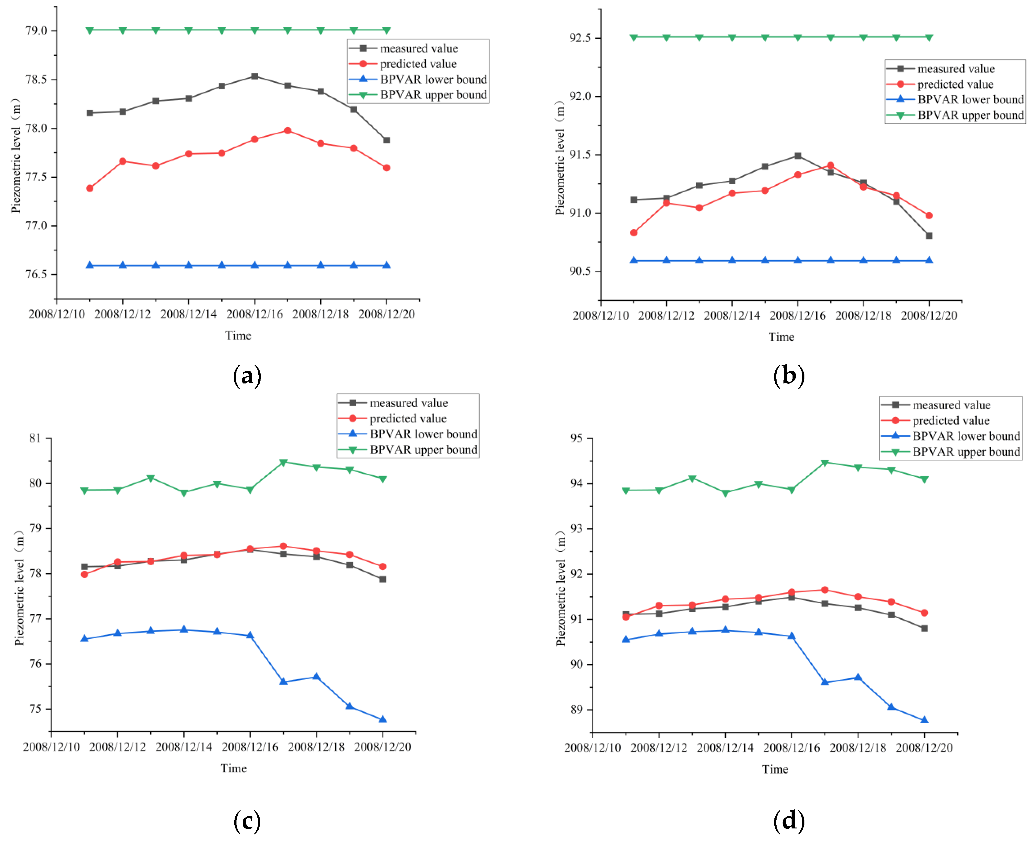
By using the Gibbs sampling method to infer the posterior distribution of the model parameters, the fitting results of the uplift pressure monitoring data are obtained from the posterior probability distribution of the model parameters. The model uses one-step advance forecasting. For the case of no exogenous variables, the forecast result is calculated according to Equation (25), and it consists mainly of two parts: endogenous variables and the residual vector. The number of lag terms of endogenous variables is calculated by the optimal lag order determined. For the presence of exogenous variables, the forecast result is calculated according to Equation (26) and is composed of three parts: endogenous variables, exogenous variables, and residual vectors. The number of lag terms of endogenous variables is determined by the optimal lag order. The prediction interval of the BPVAR model represents a 95% confidence interval.

Figure 2. Flowchart of the construction of the OPTICS- and BPVAR-based concrete dam uplift pressure safety monitoring models.

Figure 2. Flowchart of the construction of the OPTICS- and BPVAR-based concrete dam uplift pressure safety monitoring models.

4. Engineering Examples

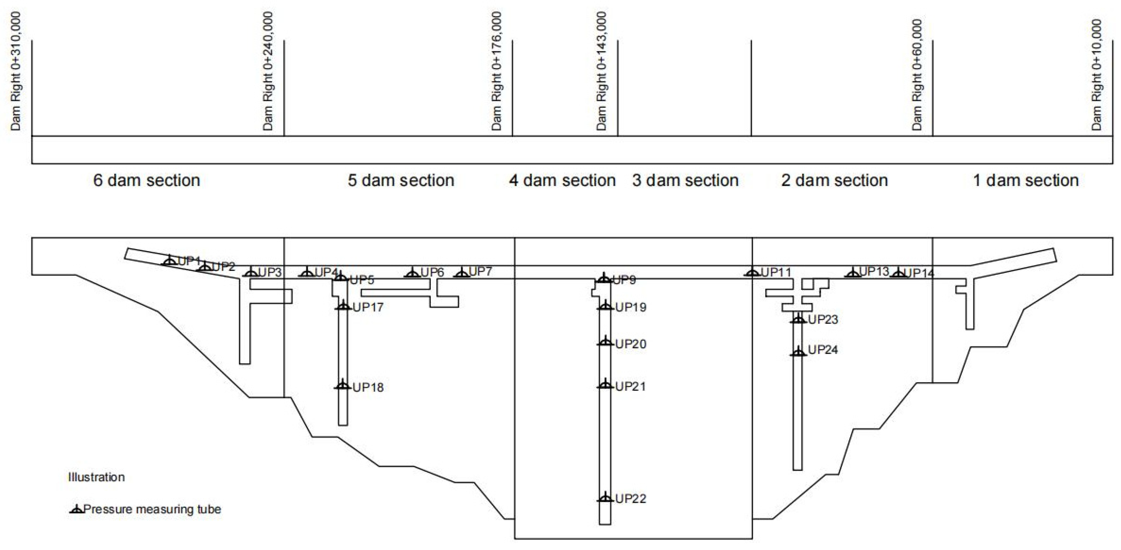
4.1. Project Overview

The water retention system of the hydropower station consists of a roller-compacted concrete gravity dam reaching a maximum height of 113.0 m, with a 308.5 m overall length of the dam crest, and a dam crest elevation of 179.0 m. Its main task is to generate electricity. The uplift pressure holes in the dam foundation are distributed in two areas: the first area is in the vertical foundation corridor, and the second area is in the horizontal corridor. The UP1~UP16 measuring points are located in the first area, and the UP17~UP25 side points are located in the second area. There are a total of 25 measuring points, as shown in Figure 3. The UP8, UP10, UP12, UP15, and UP16 measuring points lost more data and so did not appear. The values measured at all the points included manual and automated values. The period from November 2002 to November 2008 was the time series of automated monitoring, and the monitoring frequency was once a day. The dam is located in Yongding County, Fujian Province. The dam site is in the middle of the cotton beach canyon section of the main stream of the Tingjiang River. The valley of the dam site is narrow, a “V”-shaped valley with basically symmetrical terrain, and the mountains on both sides are strong. The bedrock is early Yanshanian biotite granite with medium-fine grain structure and massive structure, and the slightly weathered rock is dense and hard. There are also granite porphyry veins, diorite lamprophyre veins, and multiple sets of faults in the rock mass. The rock mass of the bank slope of the river valley is seriously weathered, except for the whole, strong, weak, and slightly weathered zones, and has the characteristics of spherical and interlayer weathering. There are many boulders left in the weathered rock, and the permeability of the rock mass is weak. The engineering geological conditions for dam construction are good.

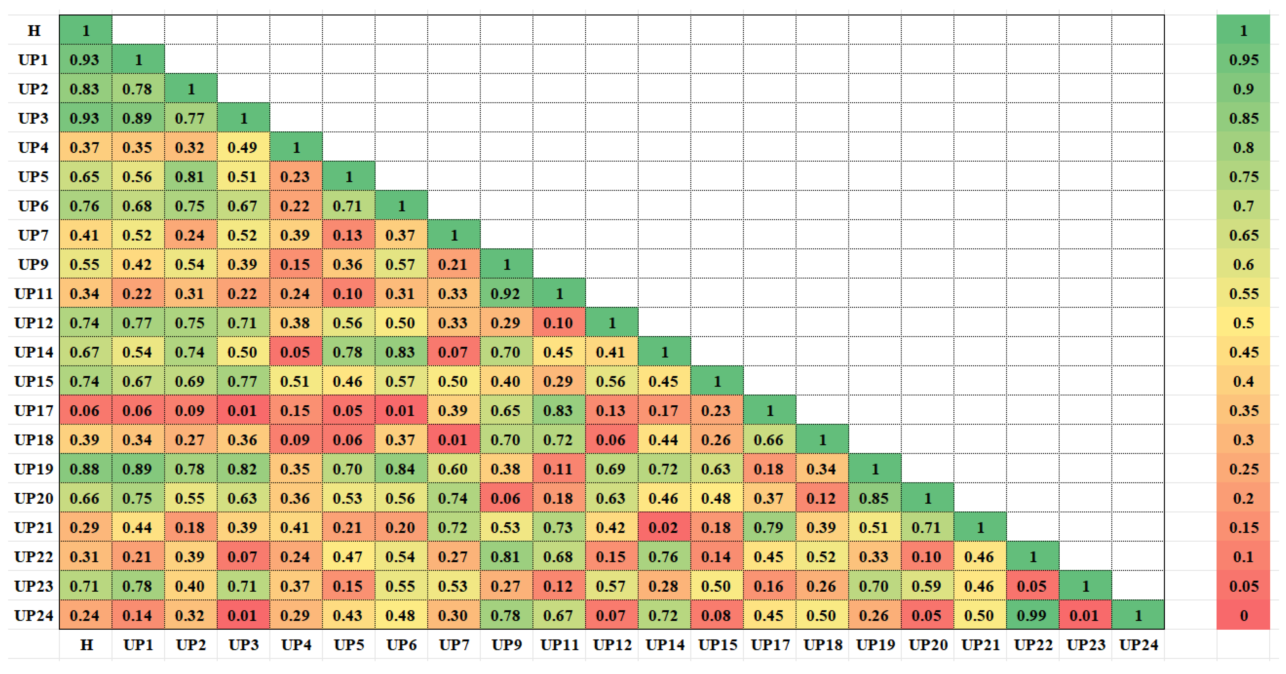
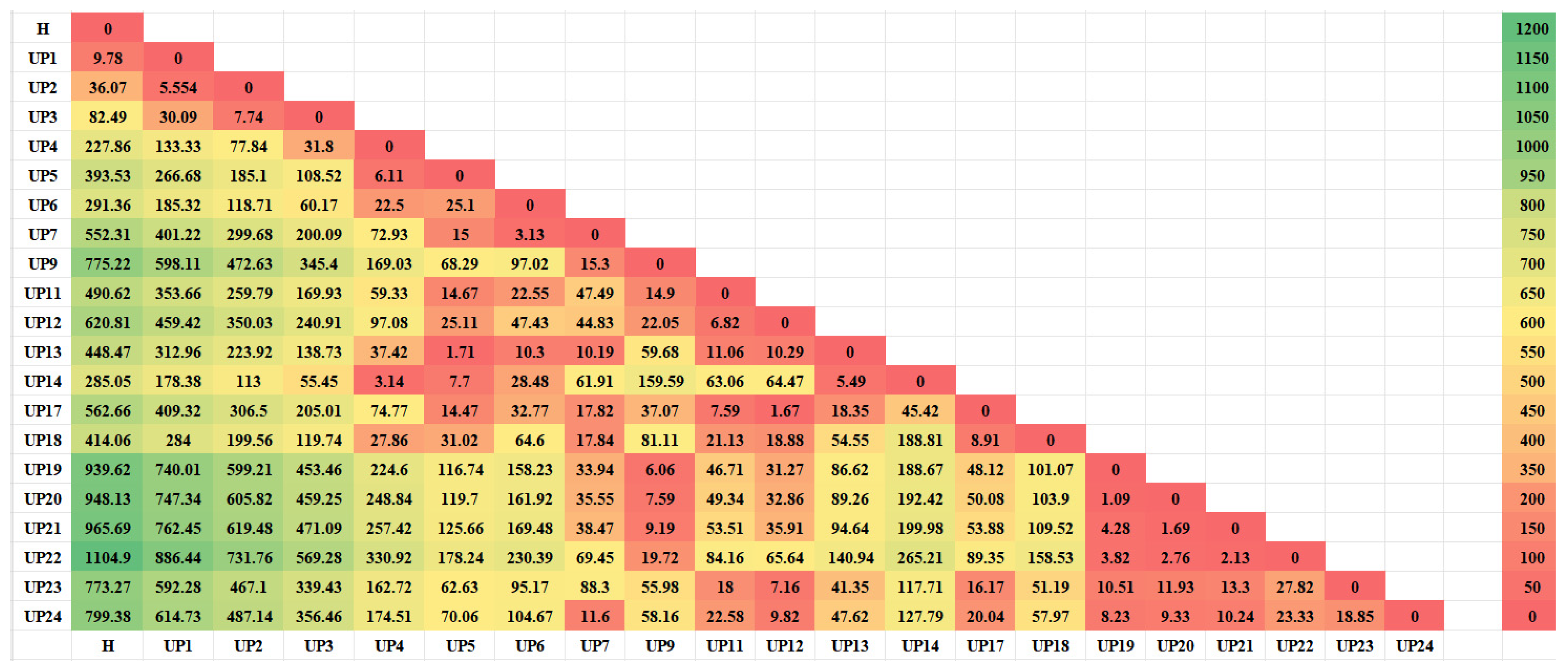
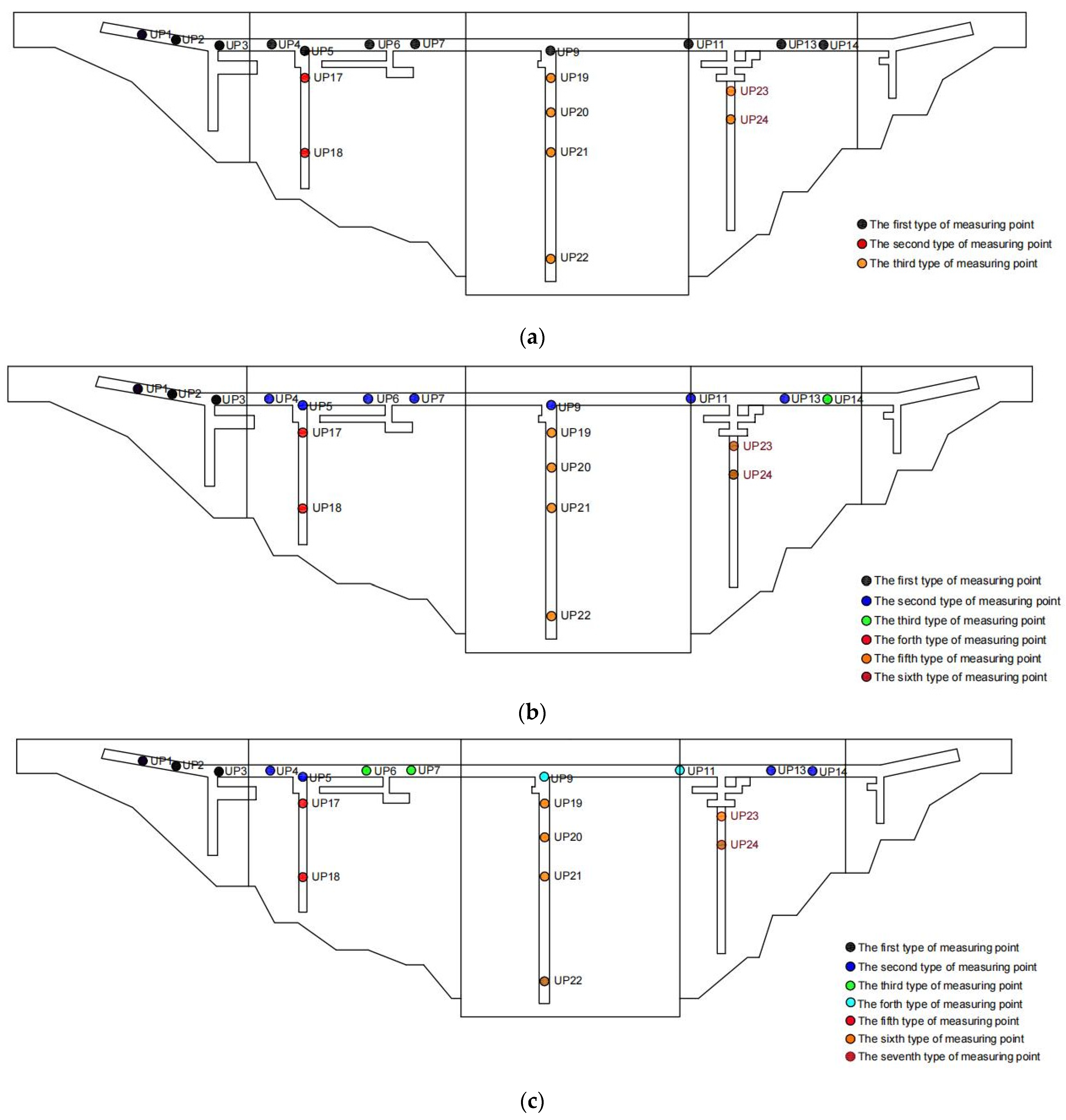
4.2. Spatial Cluster Analysis

In the above piezometric tubes, the monitoring series UP1~UP7, UP9, UP11, UP13, UP14, and UP17~UP24 cover more than one year, and the data from these measuring points are reliable. Therefore, the OPTICS clustering method was selected to spatially analyze the above 20 measuring points. For the cluster analysis, the interval was between 1 January 2004 and 31 December 2008. A total of 1553 data points for each piezometric tube were included in the cluster analysis. Figure 4 shows the correlation analysis diagram for the 20 measuring points, and Figure 5 shows the 20 measuring points. The smallest cumulative distance map of the measuring points was constructed. The uplift pressure monitoring data of the 20 piezometers were clustered by the OPTICS density clustering method using the distance matrix calculated by the three distance indicators (cosine similarity, bilateral slope distance, and DTW), and a visualization diagram of the clustering results was obtained, as shown in Figure 6.

Table 1. Cluster evaluation indicators.

Evaluation Indicators	Cosine Similarity	Bilateral Slope Distance	DTW
Silhouette coefficient	0.51	0.55	0.58
Variance ratio criterion	2684	2848	2850

lists the evaluation indicators of the three clustering results. The silhouette coefficient uses the value of −1~1, and the value of the silhouette coefficient based on the DTW distance is closest to 1. The variance ratio criterion is in the range of 0~∞, and the variance based on the DTW distance is the maximum. Therefore, overall, the clustering result based on the DTW distance was the best. Based on the results of clustering evaluation indicators, the clustering results of OPTICS based on the DTW distance prevailed in the present study when the uplift pressure measuring points of the dam foundation were divided into seven categories. The water level of the piezometer for each type of measuring point is shown in Figure 7.

Table 2. Classification of the seven types of measuring points.

Category	Instrument ID Number	Similar Reasons
Category I	UP1, UP2, UP3	The measuring point is located in front of the grouting curtain in the same dam section (dam Section 6).
Category II	UP4, UP5, UP13, UP14	The measuring point is adjacent to and arranged behind the grouting curtain.
Category Ⅲ	UP6, UP7	The measuring point is located in the same dam section (dam Section 5) and near the right bank.
Category IV	UP9, UP11	The measuring point is located in the middle section of the dam and close to the riverbed.
Category V	UP17, UP18	The measuring points are located in the same lateral corridor (5 dam sections).
Category VI	UP19, UP20, UP21, UP23	The measuring point is located in the lateral corridor and near the upstream water level.
Category VII	UP22, UP24	The measuring point is located in the lateral corridor and near downstream, which is greatly affected by the downstream water level.

is the classification table of seven types of measuring points.

4.3. BPVAR Model Construction

4.3.1. Stationary Test of Panel Data

For non-stationary panel data, the model estimation results may be biased. Therefore, before constructing the model, the unit root test should be performed on the panel data. Using the fourth type of measurement point as a reference, the data show a significant growth trend; at this time, it is a nonstationary time series. The processing method in the present study involves using the logarithmic difference in the variables, as shown in Figure 8, to convert the data into a stationary time series and then perform a stationarity test. In this study, the LLC, IPS, and ADF-Fisher tests are employed to examine the unit root of the panel data concerning uplift pressure. The specific test results are listed in

Table 3. p value of the unit root test for panel data.

Type of Measuring Point	LLC	IPS	ADF-Fisher
Category I	0.01	0.01	0.02
Category II	0.02	0.01	0.00
Category Ⅲ	0.03	0.02	0.03
Category IV	0.00	0.00	0.05
Category Ⅴ	0.02	0.01	0.09
Category VI	0.00	0.00	0.01
Category Ⅶ	0.06	0.04	0.09

. It can be seen from Table 3 that the p values are all less than 0.1, rejecting the null hypothesis of ‘nonstationary panel data’, so the panel data is stationary.

4.3.2. Selection of the Optimal Lag Order

The optimal lag order of the model was determined using the AIC, BIC, and HQIC criteria. The details are shown in

Table 4. Test of the optimal lag order for panel data.

Type of Measuring Point	Lag Order	AIC	BIC	HQIC
Category I	1	−5.26	−5.25	−5.22
	2	−6.15	−6.12	−6.08
	3	−6.22	−6.18	−6.12 *
	4	−6.25 *	−6.20 *	−6.11
Category II	1	−17.09	−17.06	−17.02
	2	−17.21	−17.16	−17.08 *
	3	−17.25 *	−17.19 *	−17.07
	4	−17.25	−17.16	−17.01
Category Ⅲ	1	−5.00	−4.96	−4.89
	2	−5.25	−5.18 *	−5.06 *
	3	−5.26 *	−5.15	−4.98
	4	−5.26	−5.12	−4.89
Category IV	1	−7.93	−7.93	−7.91
	2	−8.32	−8.31	−8.29
	3	−8.35	−8.33 *	−8.30 *
	4	−8.36 *	−8.33	−8.29
Category V	1	−6.75	−6.72	−6.68
	2	−7.08	−7.04	−6.96 *
	3	−7.11	−7.04 *	−6.93
	4	−7.13 *	−7.04	−6.89
Category VI	1	−4.71	−4.70	−4.69
	2	−4.77	−4.76	−4.74
	3	−4.79	−4.77	−4.74
	4	−4.81 *	−4.79 *	−4.75 *
Category Ⅶ	1	−3.88	−3.81	−3.80
	2	−3.87	−3.86 *	−3.84 *
	3	−3.87	−3.86	−3.83
	4	−3.86 *	−3.85	−3.81

Note: * Denotes the optimal lag order.

. The optimal hysteresis order of the first type of monitoring point, fifth type of monitoring point, and sixth type of monitoring point is fourth; the optimal hysteresis order of the second type and fourth type of monitoring point is third; and the optimal hysteresis order of the third and seventh type of measuring points is second.

4.3.3. Model Adaptation and Forecasting Analysis

This paper creates panel data consisting of identical monitoring points and uses the BPVAR model to fit and predict.

The number of pre-iterations and effective iterations of Gibbs sampling are set to 2000 and 1000, respectively. Panel data from seven types of monitoring points are partitioned into three segments: the learning set, the test set, and the verification set. The time span of the learning set is from 1 January 2004 to 10 December 2008, and includes a total of 1533 sets of data for model fitting and hyperparameter adjustment. The test set contains 10 sets of data from 11 December 2008 to 21 December 2008 to evaluate model performance and possible adjustments. The verification set covers 10 sets of data from 21 December 2008 to 31 December 2018 to verify the robustness and prediction error of the model. After debugging several times, the overall tightness of the model is determined to be 0.5, the lag attenuation parameter is 1, and the constant term is 0.

The seventh type of measuring point data is adopted, and the fitting results of the model measuring points of UP22 and UP24 are shown in Figure 9. The multiple correlation coefficients between the fitted value and the measured value are 0.98 and 0.94, respectively, and the fitting effect is good.

The prediction results of the UP22 and UP24 models with and without the addition of exogenous variables are shown in Figure 10. Each measuring point in the test set was represented by 10 data samples. The prediction error, calculated as the difference between the predicted and actual values, was evaluated for each sample in the test dataset of the model with the addition of exogenous variables roughly fluctuated at approximately 0.1 m, indicating that the prediction accuracy of the BPVAR model improved after the addition of exogenous variables.

In order to verify the accuracy of the BPVAR model prediction, a BPVAR model, BP (Back Propagation) neural network, XGBoost algorithm, and Support Vector Machine (SVM) are used to predict and analyze the uplift pressure of UP22 and UP24 measuring points, as shown in Figure 11. Based on the prediction outcomes, the BPVAR model demonstrates greater consistency between its predicted values and the actual measurements compared to the other three models. Furthermore, the predicted values fall within the 95% confidence interval, suggesting that the BPVAR model exhibits clear advantages in prediction accuracy.

To thoroughly assess the predictive accuracy of the BPVAR model, calculate and evaluate the mean absolute error, mean absolute percentage error, mean square error, and root mean square error for both the BP model, SVM model, XGBoost model, and BPVAR model. The seventh type of measuring point data is adopted; the prediction error indexes for each model are presented in

Table 5. Evaluation of model prediction accuracy.

Monitoring Point	Assessment Metrics	BPVAR	BP	SVM	XGBoost
UP22	MAE	0.114	0.848	0.228	0.125
	MSE	0.05	1.033	0.071	0.058
	MAPE	0.124	0.921	0.246	0.135
	RMSE	0.224	1.017	0.267	0.241
UP24	MAE	0.121	0.173	0.529	1.319
	MSE	0.056	0.066	0.285	1.873
	MAPE	0.149	0.191	0.586	1.473
	RMSE	0.237	0.257	0.534	1.369

. A radar chart is constructed based on the error indexes from Table 5, as shown in Figure 12. Observing the radar chart, it becomes evident that the MAE, MAPE, MSE, and RMSE of the BPVAR model surpass those of the BP model, SVM model, and XGBoost model. This highlights the superior predictive accuracy of the BPVAR model, offering valuable insights for uplift pressure prediction and analysis.

5. Conclusions

The OPTICS algorithm was used to cluster the uplift pressure measuring points, and three different distance indexes were used to calculate the distance matrix. Clustering optimization was realized according to the two clustering evaluation indexes, and the dam foundation measuring points were divided. Then, a BPVAR safety monitoring model was established for each type of measuring point. The actual engineering data was verified, and the conclusions are summarized as follows:

(1)

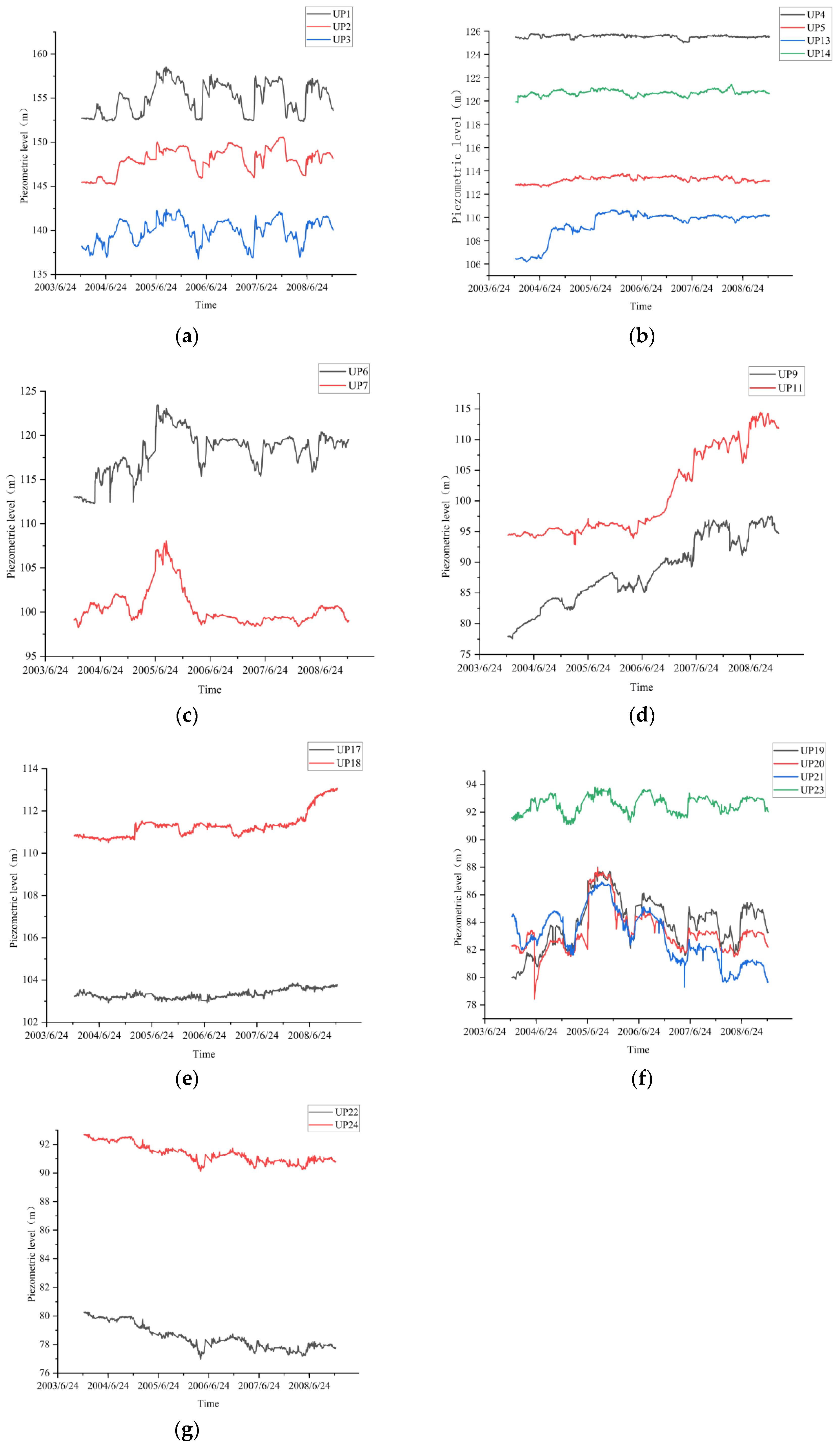
Through the calculation of the clustering evaluation index, the DTW-based clustering results among the OPTICS clustering results calculated by three different distance indicators were found to be consistent with the variation pattern of the uplift pressure monitoring value. Research on engineering applications has shown that the uplift pressure measuring points of a water conservancy project dam foundation can be divided into seven types, and the measuring points of the same type show similar variation in the law of uplift pressure.

(2)

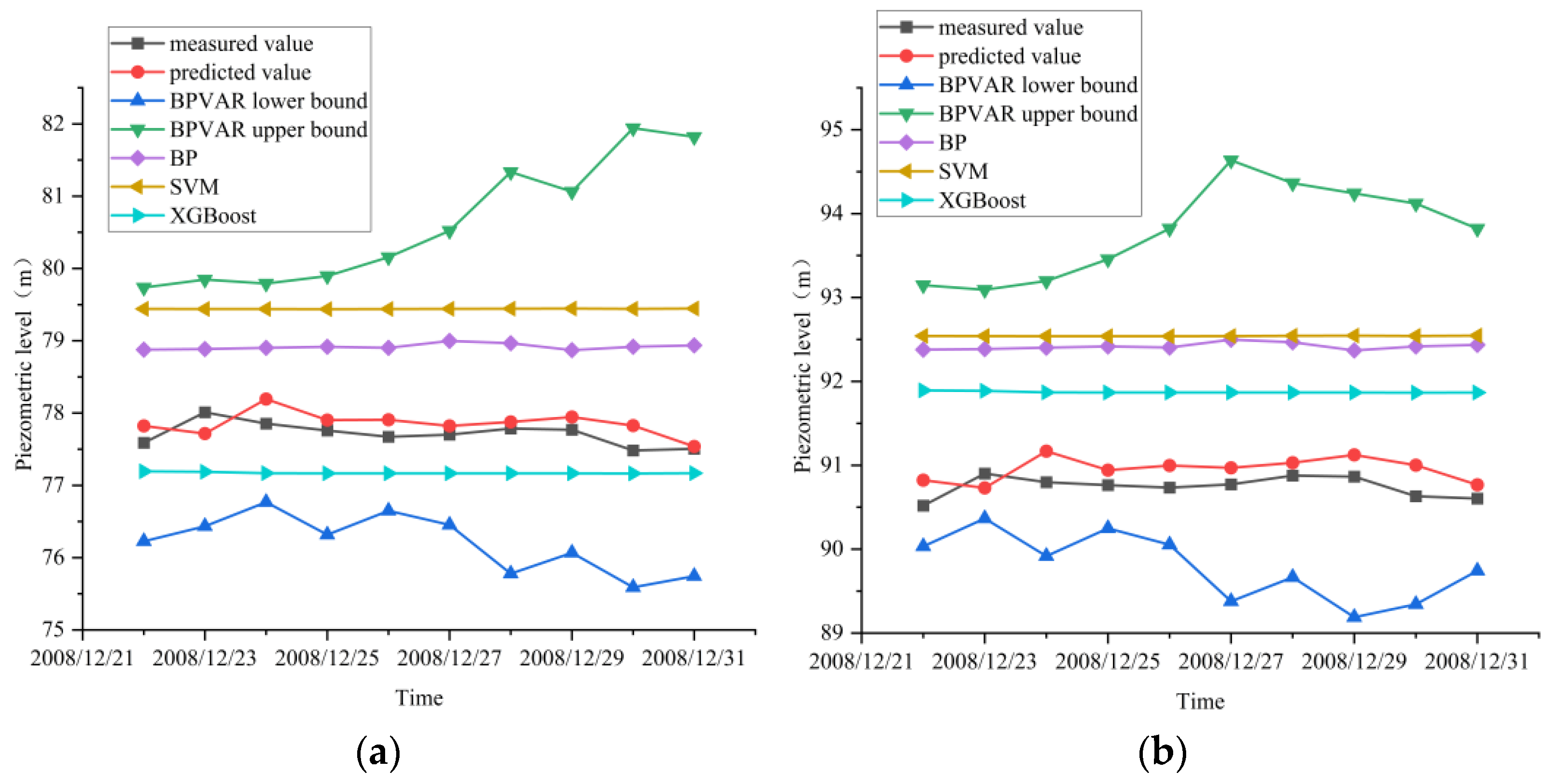
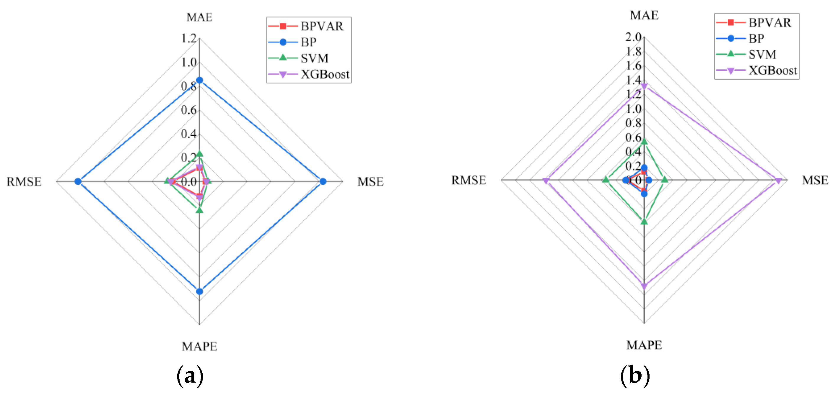
After adding exogenous variables to the BPVAR model, the multiple correlation coefficients between the fitted values and the measured values of the training set and the test set data exceeded 0.80, indicating that the modeling effect of the model was good, and the predicted uplift pressure fell within the 95% confidence interval, indicating that the BPVAR model performed well in interval prediction. The MAE, MAPE, MSE, and RMSE predicted by the BPVAR model were smaller than those of the BP model, the SVM model, and the XGBoost model.

In this study, although the BPVAR model shows good interval prediction ability, the hyperparameter values in the model are still subjective; hyperparameter values refer to the overall tightness of the model and the lag attenuation parameter. Therefore, future research will focus on finding more effective methods to determine the most accurate hyperparameters.

References

1. Wu, Z.R. Safety Monitoring Theory of Hydraulic Structures and Its Application; Higher Education Press: Beijing, China, 2003. [Google Scholar]
2. Warren, T. Roller-compacted concrete dams: A brief history and their advantages. Dams Reserv. 2012, 22, 87–90. [Google Scholar] [CrossRef]
3. Zhong, D.H.; Wang, F.; Wu, B.P.; Cui, B.; Liu, Y.X. From digital dam to smart dam. J. Hydroelectr. Power 2015, 34, 1–13. [Google Scholar]
4. Bukenya, P.; Moyo, P.; Beushausen, H.; Oosthuizen, C. Health monitoring of concrete dams: A literature review. J. Civ. Struct. Health Monit. 2014, 4, 235–244. [Google Scholar] [CrossRef]
5. Fang, C.H.; Duan, Y.H. Statistical analysis of dam—Break incidents and its cautions. Yangtze River 2010, 41, 96–101. [Google Scholar]
6. Habib, P. The Malpasset dam failure. Eng. Geol. 1987, 24, 331–338. [Google Scholar] [CrossRef]
7. Si, C.D.; Lian, J.J. Genetic support vector machine method for seepage safety monitoring of earth-rock dams. J. Hydraul. Eng. 2007, 38, 1341–1346. [Google Scholar]
8. Li, F.Q.; Qian, J.L. Application of characteristic polynomial roots of auto regression time series model in analysis of dam observation data. J. Zhejiang Univ. Eng. Sci. 2009, 43, 193–196. [Google Scholar]
9. Gu, C.; Fu, X.; Shao, C.; Shi, Z.; Su, H. Application of spatiotemporal hybrid model of deformation in safety monitoring of high arch dams: A case study. Int. J. Environ. Res. Public Health 2020, 17, 319. [Google Scholar] [CrossRef] [PubMed]
10. Wei, B.; Liu, B.; Yuan, D.; Mao, Y.; Yao, S. Spatiotemporal hybrid model for concrete arch dam deformation monitoring considering chaotic effect of residual series. Eng. Struct. 2021, 228, 111488. [Google Scholar] [CrossRef]
11. Cheng, L.; Zheng, D. Two online dam safety monitoring models based on the process of extracting environmental effect. Adv. Eng. Softw. 2013, 57, 48–56. [Google Scholar] [CrossRef]
12. Popescu, T.D.; Alexandru, A. Blind source separation: A preprocessing tool for monitoring of structures. In Proceedings of the IEEE International Conference on Automation, Quality and Testing, Robotics (AQTR), Cluj-Napoca, Romania, 24–26 May 2018. [Google Scholar]
13. Zhu, W.B.; Zhao, J.H. Application of BLS-SVM to dam safety monitoring data validation. Hydropower Autom. Dam Monit. 2009, 33, 46–50. [Google Scholar]
14. Xu, C. Research on Machine Learning Models for Health Diagnosis of Spatial Deformation Behavior of Super-High Arch Dams. Ph.D. Thesis, Changzhou University, Changzhou, China, 2020. [Google Scholar]
15. Hu, J.; Ma, F. Zoned deformation prediction model for super high arch dams using hierarchical clustering and panel data. Eng. Comput. 2020, 37, 2999–3021. [Google Scholar] [CrossRef]
16. Hu, T.Y. Spatial and temporal clustering model of concrete arch dam deformation data based on panel data analysis method. J. Yangtze River Sci. Res. Inst. 2021, 38, 39–45. [Google Scholar]
17. Wang, S.; Xu, C.; Liu, Y.; Wu, B. Mixed-coefficient panel model for evaluating the overall deformation behavior of high arch dams using the spatial clustering. Struct. Control. Health Monit. 2021, 28, e2809. [Google Scholar] [CrossRef]
18. Liu, C. Research review on vector autoregressive model for panel data. Stat. Decis. 2021, 37, 25–29. [Google Scholar]
19. Canova, F.; Ciccarelli, M. Panel vector autoregressive models: A survey. Adv. Econom. 2013, 32, 205–246. [Google Scholar]
20. Lee, S.; Karim, Z.; Khalid, N.; Zaidi, M. The spillover effects of chinese shocks on the belt and road initiative economies: New evidence using panel vector autoregression. Mathematics 2022, 10, 2414. [Google Scholar] [CrossRef]
21. Silva, F.; Sáfadi, T.; Muniz, J.; Rosa, G.; Aquino, L.; Mourão, G.; Silva, C. Bayesian analysis of autoregressive panel data model: Application in genetic evaluation of beef cattle. Sci. Agric. 2011, 68, 237–245. [Google Scholar] [CrossRef]
22. Pesaran, M. Estimation and inference in large heterogeneous panels with a multifactor error structure. Econometrica 2006, 74, 967–1012. [Google Scholar] [CrossRef]
23. Zellner, A. The Bayesian method of moments (Bmom). Adv. Econom. 1997, 12, 85–105. [Google Scholar]
24. Canova, F.; Ciccarelli, M. Forecasting and turning point predictions in a Bayesian panel VAR model. J. Econom. 2004, 120, 327–359. [Google Scholar] [CrossRef]
25. Koop, G.; Korobilis, D. Model uncertainty in panel vector autoregressive models. Eur. Econ. Rev. 2015, 81, 115–131. [Google Scholar] [CrossRef]
26. Ankerst, M.; Breunig, M.M.; Kriegel, H.P.; Sander, J. OPTICS: Ordering points to identify the clustering structure. ACM SIGMOD Rec. 1999, 28, 49–60. [Google Scholar] [CrossRef]
27. Ye, Y.J.; Du, J. Consistency loss between classification and localization based on cosine similarity. Electron. Opt. Control 2023, 30, 41–48. [Google Scholar]
28. Chen, H.D.; Chen, X.D.; Guan, J.Y.; Zhang, X.; Guo, J.J.; Yang, G.; Xu, B. A combination model for evaluating deformation regional characteristics of arch dams using time series clustering and residual correction. Mech. Syst. Signal Process. 2022, 179, 109397. [Google Scholar] [CrossRef]
29. Kamalzadeh, H.; Ahmadi, A.; Mansour, S. Clustering Time-Series by a Novel Slope-Based Similarity Measure Considering Particle Swarm Optimization. Appl. Soft Comput. 2020, 96, 106701. [Google Scholar] [CrossRef]
30. Song, K.Y.; Wang, N.B.; Wang, H.B. A Metric Learning-Based Univariate Time Series Classification Method. Information 2020, 11, 288. [Google Scholar] [CrossRef]
31. Chen, Z.; Li, H.; Zhang, X.; Sun, G.; Li, H. Risk analysis of subsea control system integration test based on K-means. China Offshore Platf. 2024, 39, 45–50. [Google Scholar]
32. He, Z.H.; Qin, W.D.; Duan, C.P. Chemical composition analysis of ancient glass products based on decision tree. In Proceedings of the 2023 International Conference on Mathematical Modeling, Algorithm and Computer Simulation (MMACS 2023), Seoul, Republic of Korea, 25–26 February 2023; Wuhan Zhicheng Times Cultural Development Co., Ltd.: Wuhan, China, 2023; Volume 9. [Google Scholar]
33. Chen, Q. Advanced Econometrics and Stata Applications; Higher Education Press: Beijing, China, 2014. [Google Scholar]
34. Levin, A.; Lin, C.; Chu, C. Unit root tests in panel data: Asymptotic and finite-sample properties. J. Econom. 2002, 108, 1–24. [Google Scholar] [CrossRef]
35. Im, K.; Pesaran, M.; Shin, Y. Testing for unit roots in heterogeneous panels. J. Econom. 2003, 115, 53–74. [Google Scholar] [CrossRef]
36. Wang, Z.; Nie, X. Unit root test and growth convergence of panel data. Stat. Decis. 2006, 2006, 19–22. [Google Scholar]
37. Choi, I. Unit root tests for panel data. J. Int. Money Financ. 2001, 20, 249–272. [Google Scholar] [CrossRef]
38. Li, J.; Ma, Z.Y.; Chen, B.F.; Li, X.J.; Zhou, F. Effect analysis of 2 m temperature correction in Xinyu city by moving average method. Meteorol. Hydrol. Mar. Instrum. 2022, 39, 43–46. [Google Scholar]
39. Akaike, H. A New Look at Statistical Model Identification. IEEE Trans. Autom. Control. 1974, 19, 716–723. [Google Scholar] [CrossRef]
40. Schwarz, G. Estimating the Dimension of a Model. Ann. Stat. 1978, 6, 461–464. [Google Scholar] [CrossRef]
41. Hannan, E.; Quin, G. The determination of the order of an autoregression. J. R. Stat. Soc. 1979, 41, 190–195. [Google Scholar] [CrossRef]
42. Zellner, A.; Hong, C. Forecasting international growth rates using Bayesian shrinkage and other procedures. J. Econom. 1989, 40, 183–202. [Google Scholar] [CrossRef]
43. Jarocinski, M. Responses to monetary policy shocks in the east and the west of Europe: A comparison. J. Appl. Econom. 2010, 25, 833–868. [Google Scholar] [CrossRef]
44. Cui, J. Research on Structural Damage Identification Based on Sparse Bayesian Learning and GIBBS Sampling; Harbin Institute of Technology: Harbin, China, 2017. [Google Scholar]
Figure 1. Schematic of the core distance and reachable distance.
Water 16 01190 g001
Figure 3. Arrangement of uplift pressure observation points in the lateral corridor.
Water 16 01190 g003
Figure 4. Similarity matrix.
Water 16 01190 g004
Figure 5. Diagram of the cumulative distance.
Water 16 01190 g005
Figure 6. OPTICS clustering results for the uplift pressure measuring points on the dam foundation. (a) Based on the cosine similarity; (b) based on the bilateral slope distance; (c) based on the DTW distance.
Water 16 01190 g006
Figure 7. Changes in the water level at the seven measuring points. (a) Category I; (b) category II; (c) category III; (d) category IV; (e) category V; (f) category VI; (g) category VII.
Water 16 01190 g007
Figure 8. Logarithmic difference diagram.
Water 16 01190 g008
Figure 9. Fitting results for the seventh type of measuring point. (a) Fitting results of UP22 measuring points; (b) fitting results of UP24 measuring points.
Water 16 01190 g009
Figure 10. Prediction results for the seventh type of measuring point. (a) UP22 measuring point prediction results (without adding exogenous variables); (b) UP24 measuring point prediction results (without adding exogenous variables); (c) UP22 measuring point prediction results (exogenous variables added); (d) UP24 measuring point prediction results (exogenous variables added).
Water 16 01190 g010
Figure 11. Model validation results for the seventh type of measuring point. (a) UP22; (b) UP24.
Water 16 01190 g011
Figure 12. Radar diagram of prediction errors for the seventh type of surveying point. (a) UP22 measuring point prediction error radar chart; (b) UP24 measuring point prediction error radar chart.
Water 16 01190 g012