
Scour, Velocities and Pressures Evaluations Produced by Spillway and Outlets of Dam


Abstract
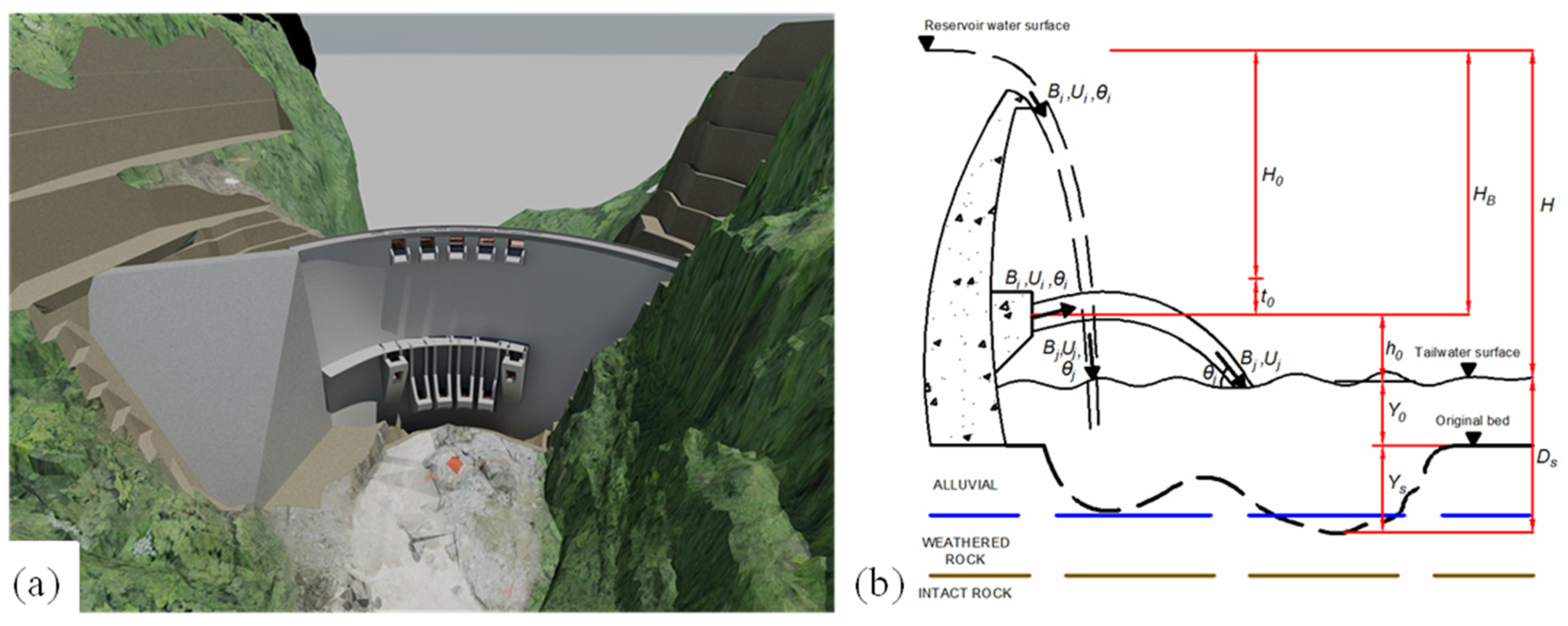
:1. Dam Characteristic
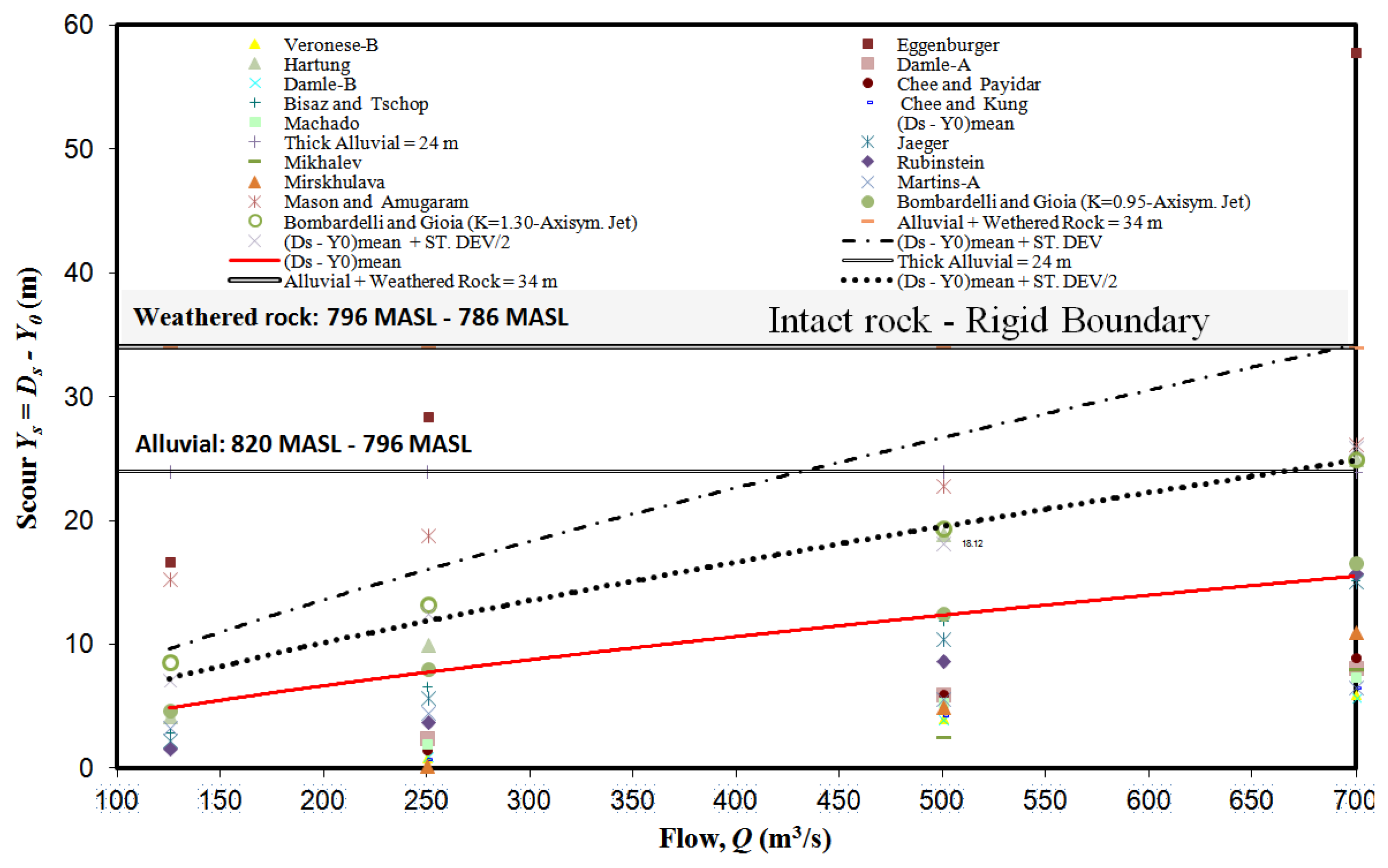
2. Empirical Formulae
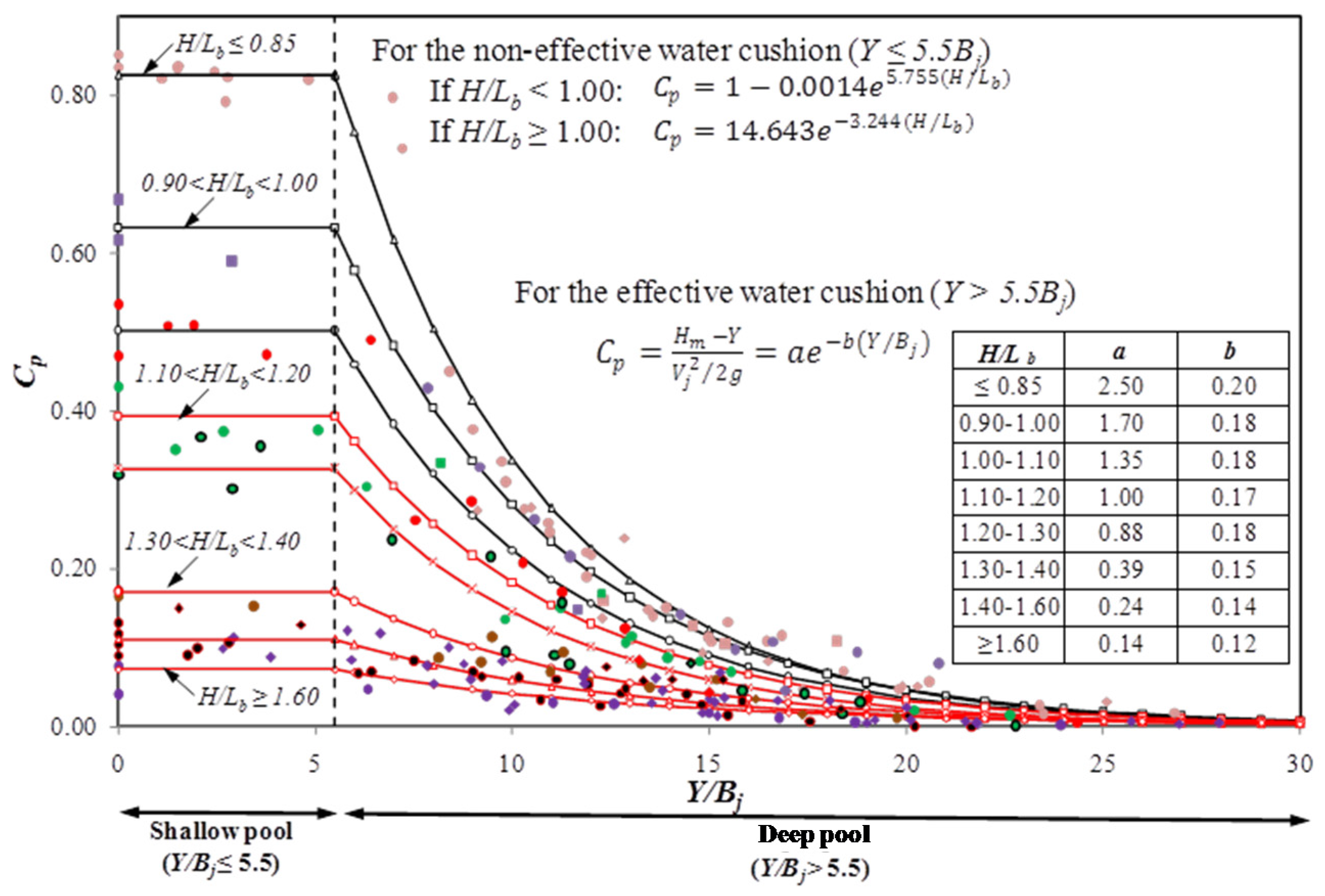
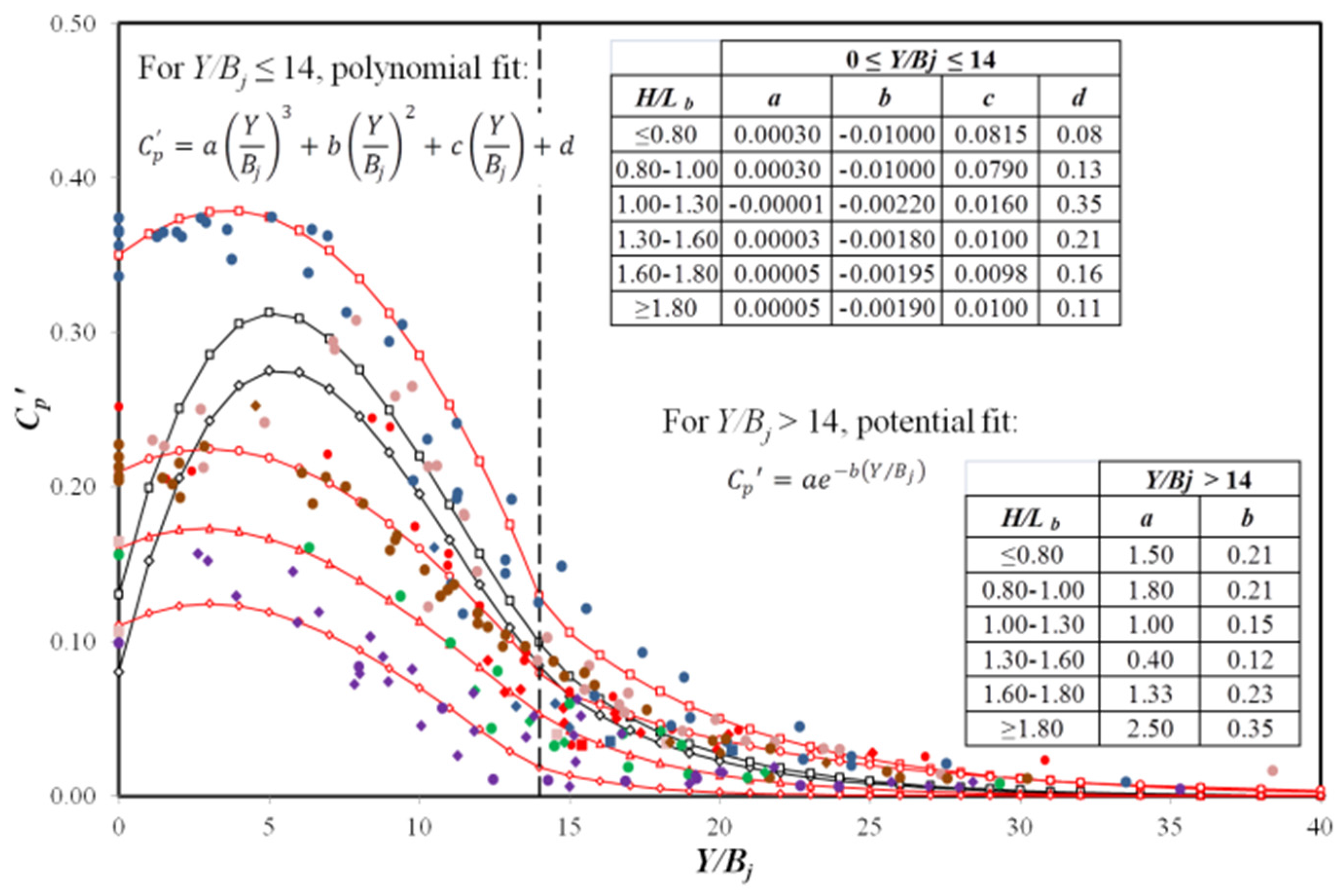
3. Semi-Empirical Methodology
4. Numerical Simulation
5. Conclusions
Acknowledgments
Author Contributions
Conflicts of Interest
Abbreviations
| A | jet area on the impact surface; |
| Bg | thickness of the jet due to gravity effect; |
| Bi | thickness of the jet in initial condition; |
| Bj | thickness of the jet in the impingement conditions; |
| CD,i | drag coefficient for sediment species i; |
| Cp | mean dynamic pressure coefficient; |
| Cp′ | fluctuating dynamic pressure coefficient; |
| Cr | coefficient of relative density; |
| crough | proportional constant of local mean grain diameter in packed sediment (default value 1.0); |
| cs,i | concentration of the suspended sediment, |
| Ds | scour depth below tailwater level; |
| d | characteristic particle diameter; |
| di | characteristic size of bed material in which i % is smaller in weight; |
| d50,packed | local mean grain diameter in packed sediment: |
| ds,i | diameter of sediment species i; |
| dm | average particle size of the bed material; |
| d∗ | dimensionless particle diameter; |
| f | residual friction angle of the granular earth material; |
| fb,i | volume fraction of sediment i in the bed-load layer; |
| fs | total volume fraction of sediment; |
| fs,i | volume fraction of sediment species i; |
| F | reduction factor of the fluctuating dynamic pressure coefficient; |
| F | body and viscous forces; |
| g | gravitational acceleration; |
magnitude of the gravitational vector; | |
| H | fall height; |
| Hn | net energy head; |
| h | energy head at the crest weir; |
| h0 | vertical distance between the outlet exit and the tailwater level; |
| Ja | join wall alteration number; |
| Jn | join set number; |
| Jr | joint wall roughness number; |
| Js | number of structure relative of the grain; |
| Jx, Jy, Jz | discontinuity spacing; |
| K | erodibility index; |
| Kb | number of the block size; |
| Kd | number of resistance to shear strength on the discontinuity contour; |
| Ki | coefficient of quadratic drag for species i; |
| Kφ | experimental parameter; |
| ks | Nikuradse roughness of the bed surface; |
| Lb | disintegration height; |
| Ms | number of resistance of the mass; |
| ns | outward pointing normal to the packed bed interface; |
| P | relative capacity of the material to resisting erosion; |
| Pjet | stream power per unit of area; |
| Pr | pressure; |
| Q | flow; |
| Qi | flow with return period i; |
| q | specific flow; |
| qbi | volumetric bed-load transport rate per unit width; |
| Re | Reynolds number; |
dimensionless parameter to computing the critical Shields number; | |
| RQD | rock quality designation; |
| SD | Standard deviation; |
| SPT | standard penetration test; |
| TR | return period; |
| t0 | energy loss in the duct; |
| Ui | velocity of the jet in the initial condition; |
| Uj | velocity of the jet in the impingement conditions; |
mean velocity of the fluid-sediment mixture; | |
direction of the fluid-sediment mixture adjacent to the packed interface; | |
| ubedload,i | velocity magnitude of bed-load; |
| ubedload,i | vector velocity of bed-load; |
| udrift,i | velocity of the sediment due to drift; |
| uf | fluid velocity; |
| ulift,i | entrainment lift velocity of sediment; |
| ur,i | relative velocity between the velocity of sediment species i and the fluid velocity; |
| usettling,i | velocity magnitude of settling; |
| us,i | velocity of sediment species i; |
drift velocity to account for particle/particle interactions; | |
| UCS | unconfined compressive strength; |
| x, y, z, v, w | empirical exponents defined by regression or optimization; |
| Y | water cushion depth; |
| Y0 | tailwater depth; |
| Ys | scour depth below the original bed; |
| αi | entrainment parameter (recommended value 0.018); |
| β | air-water relationship; |
| βi | proportionality constant of Meyer-Peter and Müller equation; |
| Γ | experimental coefficient; |
| γ | specific weight of water; |
| γr | reference unit weight of rock (27·103 N/m3); |
| δi | bed-load thickness; |
| ζ0 | Richardson-Zaki coefficient; |
| ζuser | coefficient of Richardson-Zaki coefficient (default value 1.0); |
| ζ | exponent of Richardson-Zaki relation; |
| θi | local Shields number based on the local shear stress, angle of the jet in the initial conditions; |
| θj | angle of the jet in the impingement conditions; |
dimensionless critical Shields parameter; | |
dimensionless critical Shields parameter for sloping surfaces to include the angle of repose; | |
| μf | dynamic viscosity of fluid; |
| ξ | jet lateral spread distance due to the turbulence effect; |
| ρ | water density; |
density of fluid-sediment mixture; | |
| ρr | mass density of the rock; |
| ρs | density of sediment; |
| ρs,i | density of the sediment species i; |
| τ | shear stress; |
| Φi | dimensionless bed-load transport rate; |
| φ | parameter (φ = KφTu); |
| φ | residual friction angle of the granular earth material. |
References
- Consorcio PCA. FASE B: Informe de Factibilidad, Anexo 6, Hidráulica; Consorcio PCA: Quito, Ecuador, 2012. (In Spanish) [Google Scholar]
- Schoklitsch, A. Kolkbildung unter Über-fallstrahlen. Wasserwirtschaft 1932, 25, 341–343. (In German) [Google Scholar]
- Veronese, A. Erosioni di fondo a valle di uno scarico. Ann. Lavori Pubblici 1937, 75, 717–726. (In Italian) [Google Scholar]
- Eggenberger, W. Die Kolkbildung Bei Einem Uberstromen und Bei Der Kombination Uberstromen-Unterstromen. Ph.D. Thesis, ETH Zürich, Zurich, Switzerland, 1943. [Google Scholar]
- Taraimovich, I.I. Deformation of channels below high-head spillways on rock foundations. J. Power Technol. Eng. 1978, 12, 917–923. [Google Scholar] [CrossRef]
- INCYTH-LHA. Estudio Sobre Modelo del Aliviadero de la Presa Casa de Piedra, Informe Final; DOH-044-03-82; Laboratorio de Hidráulica-Instituto Nacional del Agua: Ezeiza, Argentina, 1982. (In Spanish) [Google Scholar]
- Mason, P.J. Effects of air entrainment on plunge pool scour. J. Hydraul. Eng. 1989, 115, 385–399. [Google Scholar] [CrossRef]
- Liu, P. A new method for calculating depth of scour pit caused by overflow water jets. J. Hydraul. Res. 2005, 43, 695–701. [Google Scholar] [CrossRef]
- Bombardelli, F.A.; Gioia, G. Scouring of granular beds by jet-driven axisymmetric turbulent cauldrons. Phys. Fluids 2006, 18, 88–101. [Google Scholar] [CrossRef]
- Suppasri, A. Hydraulic Performance of Nam Ngum 2 Spillway; Asian Institute of Technology: Pathumthani, Thailand, 2007. [Google Scholar]
- Pagliara, S.; Amidei, M.; Hager, W.H. Hydraulics of 3D Plunge Pool Scour. J. Hydraul. Eng. 2008, 134, 1275–1284. [Google Scholar] [CrossRef]
- Hartung, W. Die Kolkbildung hinter Uberstromen wehren im Hinblick auf eine beweglich Sturzbettgestaltung. Die Wasser Wirtsch. 1959, 49, 309–313. (In German) [Google Scholar]
- Chee, S.P.; Padiyar, P.V. Erosion at the base of flip buckets. Eng. J. Can. 1969, 52, 22–24. [Google Scholar]
- Bisaz, E.; Tschopp, J. Profundidad de erosión al pie de un vertedero para la aplicación de corrección de arroyos en quebradas empinadas. In Proceedings of the Fifth Congreso Latinoamericano de Hidráulica (IAHR), Lima, Peru, 23–28 October 1972; pp. 447–456. (In Spanish)
- Martins, R. Scouring of rocky riverbeds by free-jet spillways. Int. Water Power Dam Constr. 1975, 27, 152–153. [Google Scholar]
- Machado, L.I. O Sistema de Dissipacao de Energia Proposto para a Barragem de Xingo. In Transactions of the International Symposium on the Layout of Dams in Narrow Gorges; ICOLD: Rio de Janeiro, Brazil, 1982. [Google Scholar]
- Jaeger, C. Uber die Aehnlichkeit bei flussaulichen Modellversuchen. Wasserkr. Wasserwirtsch. 1939, 34, 269. (In German) [Google Scholar]
- Rubinstein, G.L. Laboratory Investigation of Local Erosion on Channel Beds Below High Overflow Dams. Trans Coordinating Conferences on Hydraulic Engineering Iss VII Conference on Hydraulics of High Head Water Discharge Structures; Gosenergoizdat: Moscow, Russia, 1963. [Google Scholar]
- Mirtskhulava, T.E. Alguns Problemas da Erosao nos Leitos dos Rios. Moscow. Trans. No 443do; Laboratório Nacional de Engenharia Civil: Lisbon, Portugal, 1967. (In Portuguese) [Google Scholar]
- Ervine, D.A.; Falvey, H.R. Behavior of turbulent jets in the atmosphere and plunge pools. ICE Proc. 1987, 83, 295–314. [Google Scholar]
- Ervine, D.A.; Falvey, H.R.; Whiters, W. Pressure Fluctuations on Plunge Pool Floors. J. Hydraul. Res. 1997, 35, 257–259. [Google Scholar] [CrossRef]
- Castillo, L.G. Aerated jets and pressure fluctuation in plunge pools. In Proceedings of the 7th International Conference on Hydroscience and Engineering, Philadelphia, PA, USA, 10–13 September 2006.
- Castillo, L.G.; Puertas, J.; Dolz, J. Discussion about Scour of rock due to the impact of plunging high velocity jets Part I: A state-of-the-art review. J. Hydraul. Res. 2007, 45, 853–858. [Google Scholar] [CrossRef]
- Bollaert, E.F.R.; Schleiss, A. Scour of rock due to the impact of plunging high velocity jets. Part 1: A state-of-the-art review. J. Hydraul. Res. 2003, 41, 451–464. [Google Scholar] [CrossRef]
- Castillo, L.G.; Carrillo, J.M. Scour estimation of the Paute-Cardenillo Dam. In Proceedings of the International Perspectives on Water Resources & the Environment, Quito, Ecuador, 8–10 January 2014.
- Castillo, L.G.; Carrillo, J.M. Characterization of the dynamic actions and scour estimation downstream of a dam. In Dam Protections against Overtopping and Accidental Leakage; CRC Press: Madrid, Spain, 2015; pp. 231–243. [Google Scholar]
- Castillo, L.G.; Carrillo, J.M.; Blázquez, A. Plunge pool mean dynamic pressures: A temporal analysis in nappe flow case. J. Hydraul. Res. 2015, 53, 101–118. [Google Scholar] [CrossRef]
- Castillo, L.G.; Carrillo, J.M.; Sordo-Ward, A. Simulation of overflow nappe impingement jets. J. Hydroinform. 2014, 16, 922–940. [Google Scholar] [CrossRef]
- Federal Emergency Management Agency. FEMA P-1015, Technical Manual: Overtopping Protection for Dams. Best Practices for Design, Construction, Problem Identification and Evaluation, Inspection, Maintenance, Renovation, and Repair. Available online: https://www.fema.gov/es/media-library/assets/documents/97888 (accessed on 5 December 2014).
- Annandale, G.W. Erodibility. J. Hydraul. Res. 1995, 33, 471–494. [Google Scholar] [CrossRef]
- Annandale, G.W. Scour Technology: Mechanics and Engineering Practice; McGraw-Hill: New York, NY, USA, 2006. [Google Scholar]
- Consorcio PCA. FASE B: Informe de Factibilidad, Anexo 8, Geotécnica; Consorcio PCA: Quito, Ecuador, 2012. (In Spanish) [Google Scholar]
- Meyer-Peter, E.; Müller, R. Formulas for Bed-Load Transport. In Proceedings of the Second Meeting, International Association for Hydraulic Structures Research, Stockholm, Sweden, 7 June 1948; pp. 39–64.
- Mastbergen, D.R.; Van den Berg, J.H. Breaching in fine sands and the generation of sustained turbidity currents in submarine canyons. Sedimentology 2003, 50, 625–637. [Google Scholar] [CrossRef]
- Brethour, J.; Burnham, J. Modeling Sediment Erosion and Deposition with the FLOW-3D Sedimentation & Scour Model; Flow Science Technical Note, FSI-10-TN85; Flow Science, Inc.: Santa Fe, Mexico, 2010; pp. 1–22. [Google Scholar]
- Hirt, C.W.; Nichols, B.D. Volume of Fluid (VOF) Method for the Dynamics of Free Boundaries. J. Comput. Phys. 1981, 39, 201–225. [Google Scholar] [CrossRef]
- Flow Science, Inc. FLOW-3D Users Manual Version 11.0; Flow Science, Inc.: Santa Fe, Mexico, 2014. [Google Scholar]
- Richardson, J.F.; Zaki, W.N. Sedimentation and fluidization (Part I). Trans. Inst. Chem. Eng. 1954, 32, 35–53. [Google Scholar]
- Soulsby, R. Chapter 9: Bedload transport. In Dynamics of Marine Sand; Thomas Telford Publications: London, UK, 1997. [Google Scholar]
- Van Rijn, L. Sediment transport, Part I: Bed load transport. J. Hydraul. Eng. 1984, 110, 1431–1456. [Google Scholar] [CrossRef]
- Castillo, L.G.; Carrillo, J.M.; Álvarez, M.A. Complementary Methods for Determining the Sedimentation and Flushing in a Reservoir. J. Hydraul. Eng. 2015, 141, 05015004. [Google Scholar] [CrossRef]


| Bed Material | D16 (m) | D50 (m) | D84 (m) | D90 (m) | Dm (m) |
|---|---|---|---|---|---|
| Alluvial (820 MASL to 796 MASL) | 0.006 | 0.150 | 0.225 | 0.240 | 0.124 |
| Weathered rock (796 MASL to 786 MASL) | 0.045 | 0.160 | 0.500 | 0.550 | 0.235 |
| Author | Γ | v | w | x | y | z | d |
|---|---|---|---|---|---|---|---|
| Hartung [12] | 1.400 | 0 | 0 | 0.64 | 0.360 | 0.32 | d85 |
| Chee and Padiyar [13] | 2.126 | 0 | 0 | 0.67 | 0.180 | 0.063 | dm |
| Bisaz and and Tschopp [14] | 2.760 | 0 | 0 | 0.50 | 0.250 | 1.00 | d90 |
| Martins-A [15] | 1.500 | 0 | 0 | 0.60 | 0.100 | 0.00 | - |
| Machado [16] | 1.350 | 0 | 0 | 0.50 | 0.3145 | 0.0645 | d90 |
| Author (Year) | Formulae | Parameters |
|---|---|---|
| Jaeger [17] | dm = average particle size of the bed material d90 = bed material size, 90% is smaller in weight θT = impingement jet angle g = gravitational acceleration (9.81 m/s2) β = air-water relationship ρ = water density ρs = density of sediment Γ = experimental coefficient | |
| Rubinstein [18] | ||
| Mirskhulava [19] | ||
| Mason [7] | ||
| Bombardelli and Gioia [9] | Axisymmetric jet: |
| Material | Formulae | Parameters |
|---|---|---|
| Rock | UCS = unconfined compressive strength Cr = coefficient of relative density ρr = mass density of the rock g = gravitational acceleration γr = reference unit weight of rock (27·103 N/m3) | |
| Non-cohesive granular soil | The relative magnitude is obtained by means of the standard penetration test (SPT). When the SPT value exceeds 80, the non-cohesive granular material is taken as rock. | |
| Rock | RQD = rock quality designation RQD = values range between 5 and 100 Jn = values range between 1 and 5 Kb = values range between 1 and 100 Jn = join set number | |
| Non-cohesive granular soil | d = characteristic particle diameter (m) | |
| Rock | Jr = joint wall roughness number Ja = join wall alteration number | |
| Non-cohesive granular soil | = residual friction angle of the granular earth material | |
| Variable | Value |
|---|---|
| Angle of rock friction, SPT (°) | 38 |
| Specific weight (kN/m3) | 27.64 |
| Unconfined compress. resistant, UCS (MPa) | 50 |
| Relative density coefficient, Cr | 1.024 |
| RQD (calculated) | 82.66 |
| Number of join system (calculated), Jn | 1.83 |
| Discontinuity spacing, Jx, Jy, Jz (m) | 0.5 |
| Average block diameter (calculated), (m) | 0.5 |
| Roughness degree, Jr | 2 |
| Alteration degree, Ja | 1 |
| Variable | Alluvial | Weathered Rock | Intact Rock | Concrete |
|---|---|---|---|---|
| Ms | 0.19 | 0.41 | 51.19 | 20.47 |
| Kb | 11.39 | 125 | 49.18 | 49.18 |
| Kd | 0.78 | 0.78 | 2.00 | 5.33 |
| Js | 1.00 | 1.00 | 0.60 | 1.00 |
| Erodibility index, K | 1.69 | 40 | 3021 | 7280 |
| Stream power, Prock (kW/m2) | 1.50 | 16 | 408 | 788 |
| Variable | Parametric Methodology | FLOW-3D |
|---|---|---|
| Net drop height (m) | 120.00 | 120.00 |
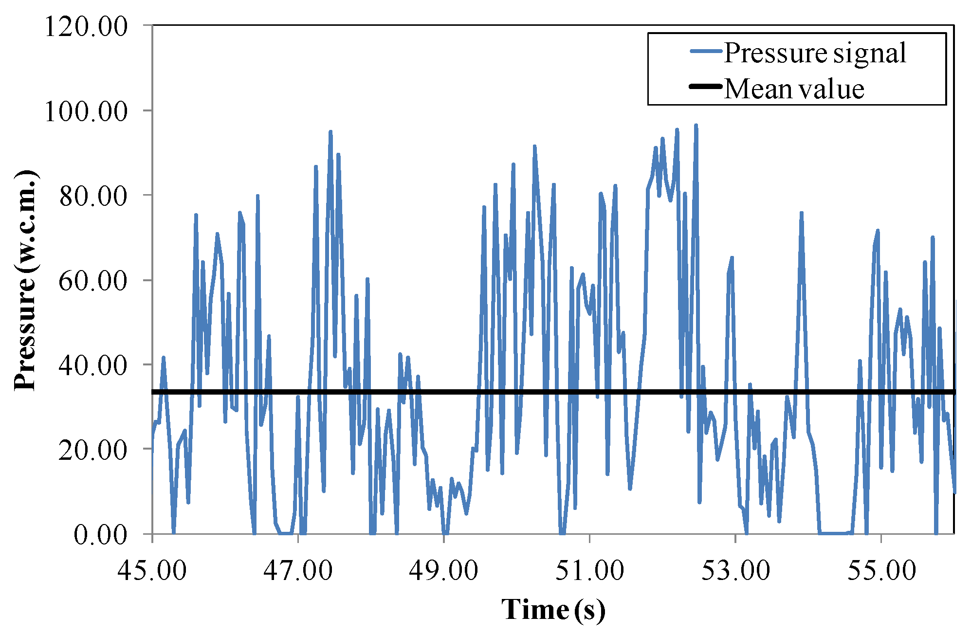
| Mean dynamic pressure (m) | 30.56 | 33.44 |
| Mean dynamic pressure coefficient, Cp | 0.28 | 0.31 |
| Relation | Formulae | Parameters |
|---|---|---|
| Drag function | ds,i and CD,i = diameter and drag coefficient for sediment species i μf = fluid dynamic viscosity ur,j = drift velocity fs = sediment total volume fraction ζ = ζuserζ0; ζuser = 1 = Reynolds number on the particle di ρf = fluid density ρs,i = density of sediment species i β = slope bed angle ϕi = repose angle for sediment species i (default is 32°) Ψ = angle between the flow and the upslope direction (flow directly up a slope Ψ = 0°) τ = local shear stress = gravitational vector αi = entrainment parameter (~0.018) ns = outward pointing normal to the packed bed interface fb,i = volume fraction of sediment i in the bed-load layer Φi = dimensionless bed-load transport (MPM) ** d* = dimensionless particle diameter = local Shields number | |
| Drift velocity correction | ||
| Richardson-Zaky coefficient | for for for for | |
| Critical Shields parameter (S-W) * | ||
| Critical Shields parameter modified for sloping surface | ||
| Local Shields number | ||
| Sediment entrainment lift velocity | ||
| Dimensionless particle diameter | ||
| Volumetric bed-load transport rate per unit width | ||
| Bed-load thickness |
| Method | Free Surface Weir Q4 = 700 m3/s | Half-Height Outlet Q40 = 1760 m3/s | ||||
|---|---|---|---|---|---|---|
| Ys (m) | Ys + 0.50SD (m) | Ys + SD (m) | Ys (m) | Ys + 0.50SD (m) | Ys + SD (m) | |
| Empirical formulations | 17 | 24 | 34 | 32 | >34 | >34 |
| Erodibility Index Pressure fluctuations | 20 | - | - | >34 | - | - |
| FLOW-3D v11 | 21 | - | - | >34 | - | - |
© 2016 by the authors; licensee MDPI, Basel, Switzerland. This article is an open access article distributed under the terms and conditions of the Creative Commons by Attribution (CC-BY) license (http://creativecommons.org/licenses/by/4.0/).
Share and Cite
Castillo, L.G.; Carrillo, J.M. Scour, Velocities and Pressures Evaluations Produced by Spillway and Outlets of Dam. Water 2016, 8, 68. https://doi.org/10.3390/w8030068
Castillo LG, Carrillo JM. Scour, Velocities and Pressures Evaluations Produced by Spillway and Outlets of Dam. Water. 2016; 8(3):68. https://doi.org/10.3390/w8030068
Chicago/Turabian StyleCastillo, Luis G., and José M. Carrillo. 2016. "Scour, Velocities and Pressures Evaluations Produced by Spillway and Outlets of Dam" Water 8, no. 3: 68. https://doi.org/10.3390/w8030068
APA StyleCastillo, L. G., & Carrillo, J. M. (2016). Scour, Velocities and Pressures Evaluations Produced by Spillway and Outlets of Dam. Water, 8(3), 68. https://doi.org/10.3390/w8030068