Analysing the Effects of Forest Cover and Irrigation Farm Dams on Streamflows of Water-Scarce Catchments in South Australia through the SWAT Model

Abstract

To assist water resource managers with future land use planning efforts, the eco-hydrological model Soil and Water Assessment Tool (SWAT) was applied to three catchments in South Australia that experience extreme low flow conditions. Particular land uses and management issues of interest included forest covers, known to affect water yields, and farm dams, known to intercept and change the hydrological dynamics in a catchment. The study achieved a satisfactory daily calibration when irrigation farm dams were incorporated in the model. For the catchment dominated by extreme low flows, a better daily simulation across a range of qualitative and quantitative metrics was gained using the base-flow static threshold optimization technique. Scenario analysis on effects of forest cover indicated an increase of surface flow and a reduction of base-flow when native eucalyptus lands were replaced by pastures and vice versa. A decreasing trend was observed for the overall water yield of catchments with more forest plantation due to the higher evapotranspiration (ET) rate and the decline in surface flow. With regards to effects of irrigation farm dams, assessment on a daily time step suggested that a significant volume of water is stored in these systems with the water loss rate highest in June and July. On an annual basis, the model indicated that approximately 13.1% to 22.0% of water has been captured by farm dams for irrigation. However, the scenario analysis revealed that the purposes of use of farm dams rather than their volumetric capacities in the catchment determined the magnitude of effects on streamflows. Water extracted from farm dams for irrigation of orchards and vineyards are more likely to diminish streamflows than other land uses. Outputs from this study suggest that the water use restrictions from farm dams during recent drought periods were an effective tool to minimize impacts on streamflows.

1. Introduction

Forecasting of streamflow provides critical information to water resource managers, local water supply authorities, and other stakeholders for adaptive management of catchments. However, streamflow modelling can be extremely challenging in catchments with semi-arid climates [1,2]. In these catchments, the amount of rainfall contribution to flows is generally low and is off-set by evapotranspiration [3,4]. Significant streamflows are usually restricted to winter months when rainfall volumes exceed evaporation [4].

Streamflows in South Australia experienced severe drought conditions in the period from 1998 to 2008 [5,6]. The consequent very low flows can seriously affect agricultural yield and the biodiversity of the system [7,8,9]. In order to protect water resources, extraction restrictions were placed on irrigation from storage water bodies, including farm dams during that time [5,10,11]. Farm dams operate as a critical component for dryland agriculture used to capture freshwater during rainy seasons in order to supply important portion of water need for irrigation [11,12]. Such restrictions on irrigation farm dams can increase the risk to the local economy as irrigated production is generally reduced and more resources are needed to carefully manage more limited water supplies [13,14]. In addition, natural catchments have a growing demand for development that further challenges the task of sustaining the quality of the water within a catchment.

To address these commonly occurring issues, some modelling tools such as Water—Community Resource Evaluation and Simulation System (WaterCress), Australian Water Balance Model (AWBM), or Source model have been developed [15,16,17]. Given the complexity of processes in catchments, there remains major concern as to the applicability of these lumped to semi-distributed models with various degrees of simplification and conceptualization of physical processes [18]. Another issue is the uncertainty associated with the input data required for modelling and the modelling processes that are not covered in these models. The challenge for local catchment managers is thus to identify a fit-for-purpose, reasonably accurate forecast tool given complex biophysical systems in a catchment, overlaid by highly variable climate scenarios, while being fully aware of data availability and the inherent uncertainties of the analysis methods.

SWAT [19] is a physically based semi-distributed model that takes spatial variations of climate, topography, land uses, and soils into account in model parameters. The model was proven as suitable for long-term analysis of hydrological processes [20,21,22,23]. Several studies of SWAT have demonstrated satisfying results when adapted to catchments with distinct climate and various geographic conditions [20,22,23]. This includes case studies of dry and variable climates [24]. Successful simulation of streamflow was provided for 29 major rivers across Europe with a broad range of semi-arid, Mediterranean, continental, oceanic, or Tundra climate [23]. Successful applications were also reported for the regions of arid climate across the U.S. [18] and Africa [25]. In the case of the driest inhabited continent of Australia [2], studies of hydrological modelling by SWAT are concentrated more in the southeastern part of the country [24] with Shrestha et al. [6] being the only known case study for South Australia.

In terms of calibration and validation of the SWAT models, there is no single criteria favoured for judging the model performance [21,22]. Most published SWAT applications that focus on hydrology use both graphical and statistical criteria [19,22]. Nash-Sutcliffe (NS) statistics have become increasingly used for SWAT model optimization compared to other metrics [20,22,26]. Some studies with a focus on dry time series using NS as objective functions showed both good and poor results [2,4,27,28,29,30]. A study by Saha et al. [2] achieved a satisfactory solution of NS statistical threshold at a monthly time step, but the highest value at a daily time step was 0.124 which is far below the satisfactory threshold. Study of Brown et al. [4] reached high daily NS during the calibration and validation period but failed during the period of persistent and severe drought. A significant improvement of daily NS was suggested by considering seasonal variability during model calibration [28]. Similar good results were reported when calibrating streamflow under wet and dry seasons separately in [29,30]. Since the NS efficiency metric applies to the whole simulation period, it was not recommended for application to low flow periods of streamflows [27,30].

Problems with simulating the streamflows in water limited catchments are associated with their naturally dry but also variable climate [2,8]. Along with very low flows, these catchments are characterised by extensive, extremely skewed, and exacerbated periods of no flows [14,26]. In addition to this, high flows can sporadically occur during the rainy seasons as well as from thunderstorms during the dry seasons [31]. Models for catchments dominated by low streamflows have been shown to often overestimate the low and underestimate the high flow events [2,4,6]. For long-term modelling of catchments with dominant low flows, it therefore seems to be advantageous to focus on methods that equally consider the contribution of both low and high flows as a whole rather than performing the discontinuous seasonal calibration.

In this context, this study develops and validates SWAT models for South Australian catchments that experience distinct low-to-zero streamflows. The study focuses on the research question regarding how forestry and irrigation affect simulated streamflows in South Australian catchments. Taking into account that farm dams are critical sources for irrigation of dryland agriculture, scenarios analyze the cases: (1) without farm dams; (2) with farm dams considered as natural water bodies; and (3) with farm dams to be used for irrigation.

2. Materials and Methods

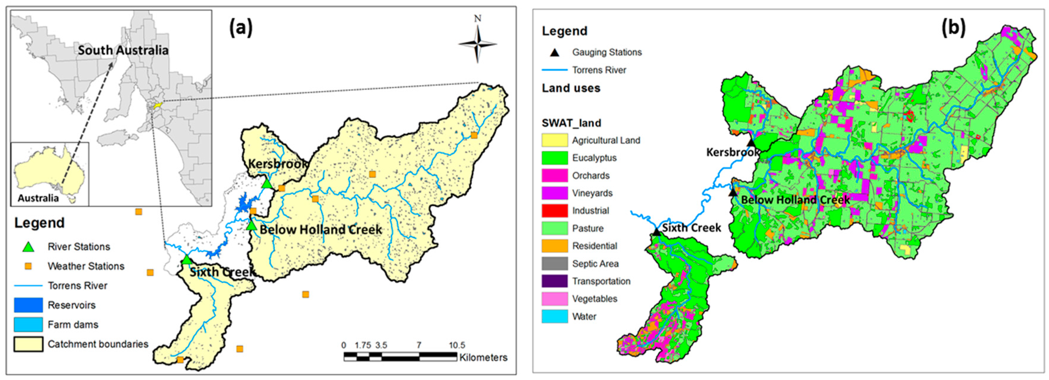
2.1. Study Area

The study area is situated 30 km north-east of Adelaide (South Australia) and covers an area of 29,640 ha with an elevation range from 200 to 710 m above sea level (Figure 1a). The climate is Mediterranean with an average annual rainfall of 585 mm [30]. Whilst its average monthly rainfall in January and February is around 20 mm, rainless months are quite common [31]. Since 2000, the climate has been in a generally drier than average cycle with declining trend in annual rainfall over the past 100 years [9,32]. This change is causing local streamflows to become more unpredictable when paired with other effects such as increasing development within the catchment [9,32].

2.2. SWAT Model Input Data

The inputs required for the study include topographic, land-use, soil, climatic, and stream flow data. Topography was defined by a digital elevation model (DEM). DEM was aggregated from a 10 m × 10 m contour interpolation that was obtained from the South Australian (SA) Water Corporation. The land use map of 2007 with a resolution of 1:100,000 provided updates on the boundaries, the locations and relative areas of protected zones, native eucalyptus forests, main agricultural lands, and water bodies (Figure 1b). A 1:100,000 soil map was provided by SA Department of State Development while a soil database of 117 soil types with detailed profile of five soil layers (Level 5 Soil Attributes) was extracted manually from the Australian Soil Resource Information System [33]. Daily climatic data from 1970 to 2014 of 10 stations were collected from the Scientific Information for Land owners (SILO) [34]. Maps and data records of streamflows in the Upper Torrens watershed were provided by the SA Water Corporation and SA Department of Environment, Water and Natural Resources (DEWNR).

Three available gauging stations in the study area include Below Holland Creek, Kersbrook, and Sixth Creek (Figure 1). The flows through these stations are the main natural sources that feed into the catchment reservoirs [11]. Apart from these, the Below Holland Creek station operates as part of the environmental flows monitoring program. As the average volume of runoff from the catchments does not meet the water demands of local communities, agriculture, and mining (Figure 1b and Figure 2), water is diverted from the River Murray via the Mannum to the Adelaide pipeline as required rather than only during the driest periods [7,11].

2.3. SWAT Model Set-Up

The semi-distributed model SWAT (ArcSWAT version 2012) [35] was used to model the three catchments in this study. To characterize the three catchments, the threshold value of 200 ha was applied which resulted in the delineation of the Kersbrook, Sixth Creek, and Below Holland Creek catchments into 7, 9, and 31 sub-basins respectively. Unique combinations of land-uses, soil types, and slopes were aggregated to form the Hydrologic Response Units (HRU) using the percentage threshold method. In this step, the relatively small areas of horticulture, viticulture, and vegetables were exempted from the threshold dissolution to provide a realistic representation of main land uses of the catchments. The multiple HRUs option resulted in 372 HRUs for the study, which included 52, 98, and 222 HRUs for the Kersbrook, Sixth Creek, and Below Holland Creek catchments. The flows were calculated at the HRU level and then aggregated to the sub-basin scale [36].

The management operation section (.Mgt) in the SWAT edit was modified with regards to the management and irrigation practices. The default start and end of growth seasons, and auto irrigation schemes were replaced by the date’s specific operations for main horticultural practices based on information from local farmers and expert knowledge. For orchards and vineyards, the plant growth season starts in September and ends by the end of March. Meanwhile, the growth seasons for vegetables often coincide with rainy periods with two cycles from January until May and from June until the end of September. The harvest option was applied for orchards and vineyards, and harvest and kill was used for vegetables. The irrigation amounts (as specified in the next section) were scheduled to be highest before and lowest after harvesting. In the case of forests and pasture land uses, start and end of growing seasons correspond with spring and late autumn, respectively, with no irrigations applied.

The surface runoff was calculated using the Soil Conservation Service (SCS) curve number [37]. For the potential evapotranspiration (PET) calculation, the Hargreaves method [38] was used over the alternative methods as it produces closest results comparing to the PET records from SILO [34]. For flow routing into channels, the study used the variable storage method. In this study, SWAT models were run on daily time steps.

A more detailed description of the SWAT model configuration applied for this study is available in [36,39].

2.4. Farm Dams Configuration

Agriculture in the three catchments is both rain-fed and irrigated [9]. On average, 22% of water need for agricultural practices is derived from farm dams’ system, mainly for irrigation. Other water uses from farm dams include grazing land for livestock and livestock feeding but were temporarily restricted during the extreme drought years [5]. Recent investigation records approximately 1693 farm dams (Figure 1) with a storage capacity of 5957 ML within the study area [39].

Farm dams were incorporated as ponds by SWAT (

Table 1. Farm dams input with initial and modelled values in SWAT.

Model Parameters	Abbreviation	Units	Initial Values			Modelled Values
			Min	Max	Default	Min	Max	Mean
PND_FR	Fraction of sub-basin area that drains into ponds	fraction	0.00	1	0.00	0.00	1.00	0.40
PND_PSA	Surface area of ponds when filled to principal spillway	ha	0.10	20	5	0.00	30.24	7.55
PND_PVOL	Volume of water needed to fill ponds to the principal spillway	104 m3	0.00	100	25	0.00	47.04	12.14
PND_VOL	Initial volume of water in ponds	104 m3	0.00	100	0	0.00	4.70	1.21
NDTARG	Number of days to reach target storage	days	0	60	0	15	15	15

) [36,39] with the following water balance equation:

V = V_stored + V_flowin − V_flowout + V_pcp − V_evap − V_seep

(1)

in which V indicates the overall volume (m³) at the end of the day as the results of the volume V_stored at the beginning of the day, the volume of water V_flowin entering (m³) and V_flowout leaving (m³) the pond during the day, the amount of precipitation V_pcp (m³) contributed in and evaporation V_evap (m³) lost from the pond, as well as the volume of water removed as seepage flow V_seep (m³).

Since SWAT allows for considering only one pond in each sub-basin, all farm dams within a sub-basin were aggregated into one single pond. Similar to the reservoir configuration, in case of a pond, SWAT requires users to provide information on the surface area and volume at two levels, principal and emergency spillway. Because the actual rate of dams’ development is not available, the study assumes that the capacities of dams within each sub-basins remained constant over the period of available data. The surface areas and storage volumes of ponds were aggregated as the sum of all farm dams present in a sub-basin. This information was calculated using farm dams’ metadata provided by South Australian Government Data Directory (Data.SA) [40] and were assumed to be equal the maximum capacity of the pond when filled to the principal spillway. Meanwhile, initial areas and volumes of ponds were assumed to be 10% of the maxima and not completely drawn down. The parameter “Fraction of sub-basin area that drains into ponds” (PND-FR, 0-1) was used to quantify the proportion of runoff that had been captured by each pond. This parameter is dependent on the location, size, and densities of farm dams within a sub-basin. Large farm dams or those locate on-stream are assumed to capture 100% of runoff of the upstream sites while smaller off-stream dams have the runoff capture ratio less than 1.0 [11]. Surface evaporation coefficients for farm dams were set using a default ratio of 0.6.

2.5. Estimation of Irrigation Inputs

Irrigation from farm dams was incorporated in the model. Information on irrigation volume applied for various crops and land uses (ML) was obtained from survey results of the Australian Bureau of Statistics (ABS) [5]. At the catchment scale, information is collected every five years to supplement the annual records available for the broad territory of the entire South Australia and the latest records for the Adelaide region were updated in June 2015 [5].

The irrigation amount was estimated at the HRUs level with the methodology as suggested by ABS [10]. The total area and area watered for all agricultural practices were assumed to remain constant over the period of study. Areas of land were assumed to be irrigated when they contained land uses of horticulture. Irrigation from agricultural land and pasture were not included as the proportion of area watered versus total area of the lands in the period from 2004 to 2014 was small (less than 1%) [5]. Irrigation volumes were estimated from the 10-year averaged total volumes in order to quantify the irrigation rate (ML/ha) for specific land uses. This resulted in the water application rate of 5.09, 1.26, and 4.82 ML/ha for orchards, vineyards, and vegetables, respectively. The irrigation water extraction (ML) for the HRUs level was calculated on the basis of the calculated adjusted application rate (ML/ha) and the total area of horticulture land uses (ha) in each sub-basin. The timing of irrigation was based on expert knowledge. Irrigation was set from November until March for orchards and vineyards, and in the periods of April–May and August–September for vegetables. Water abstraction during the no-irrigation season was set as 0.

The extraction of irrigation was adapted in SWAT by adjusting the average daily water removal from HRUs with specific land uses in the section Edit SWAT inputs. An option of water removal from ponds (Average daily water removal from the pond (WUPND), 10⁴ m³) was used as this source for irrigation was not available in the management section of SWAT. The application of irrigation was then returned to HRUs by means of irrigation operations (Management operation (MGT_OP) = 2) from an external source option (Irrigation source (IRR_SC) = 5).

2.6. Model Evaluation

Auto-calibration was performed using the SWAT Calibration and Uncertainty Procedure (SWAT-CUP4) [4,6,24,41]. It incorporates five methods of which the Sequential Uncertainty Fitting program (SUFI2) was selected in this study. SUFI2 provides two methods for sensitivity analysis, namely one-at-a-time sensitivity analysis (OAT) and global sensitivity analysis. OAT was tested first in order to select a set of sensitive parameters from available literature [2,4,6,41,42] for the model calibration. Global sensitivity analysis is incorporated with calibration in SUFI2 and results were used to evaluate the sensitivity of selected parameters. For model calibration, NS was selected as the Objective Function of SUFI2 method.

In case the NS goal type failed to define a solution, a modified version of NS called constant base-flow separation (BFS) was also tested [41]:

$$\mathrm{NS}=1-\frac{{{\displaystyle \sum }}_i{(Q_{m,i}-Q_{s,i})}^2}{{{\displaystyle \sum }}_i{(Q_{m,i}-\overline{Q_m})}^2}$$

(2)

$$\mathrm{g}={\displaystyle \sum }_j{w}_{j}N{S}_j$$

(3)

where: Q is a variable (e.g., flow), m and s are measured and simulated value respectively, i is the i^th data, the bar stands for average, and w is the weight value of a partial variable.

The BFS method defines a threshold which allows the two parts of the flow, i.e., “above” and “below” the threshold, to have different weights during the calibration procedure. By assigning different weights, the less dominant flow part can have a higher contribution to the objective function as the dominant flow part. This approach is suggested for calibrating flows with unbalanced distribution of high and low flow parts [41].

Ten years of data were available for the study of which the three years from 2004 to 2006 was kept as a “warm-up” period. Five years’ data from 2007 to 2011 which included both the low, medium, and high rainfall periods were used for calibration. The rest of the data from 2012 to 2014 which also represents both low and high rainfall periods was retained for validation.

The model performance of streamflows was judged on the basis of graphical, statistical, and uncertainty analysis. Three quantitative statistics, including correlation coefficient (R²), Nash-Sutcliffe (NS), and percent bias (PBIAS) are commonly used in SWAT applications [21,22] and were selected for this study. According to Moriasi et al. [21], the model performance was considered satisfactory when R² and NS was greater than 0.5, and percent bias (PBIAS) ranged between ±25% as for a monthly time step’s simulation. These criteria are allowed to be relaxed when the model is applied to a daily time step [21].

An analysis of the model uncertainties was combined with model optimization in SUFI2 [4,23,42]. The uncertainties were evaluated based on the percentage of observation points bracketed by the prediction uncertainty band (p-factor), and the degree of uncertainty, calculated as an average thickness of the band divided by the standard deviation of the observed values (r-factor). The values close to 1 and below 1.5 were selected for p- and r-factors [41].

2.7. Scenario Analysis

The models were first calibrated without irrigation inputs. These were further compared with the calibrated models which incorporate irrigation farm dams to evaluate the effects of irrigation on the model performance.

The calibrated models with irrigation inputs were used as baseline (BS) for the two main scenarios. The first scenario tested the effects of land use covers by either increasing or decreasing the area of the natural eucalyptus forest with pasture land use using the land use update option (.lup) in SWAT. These are the two most dominant land uses in the area (Figure 1b) thus any potential changes in these land use will have a high probability to cause an effect on the catchment water balance [4,31]. Taking into account the role of the three catchments as the sole natural sources for water supply to the downstream reservoirs, no other land use scenarios were considered in this study.

The second scenario evaluated the streamflows with and without irrigation farm dams. The scenario of no farm dams was defined by adjusting the value of the parameter PND-FR to 0 and by removing irrigation operations. Next, the effects of farm dams in relation to irrigation were analyzed for catchments which indicated a significant effect. For this test, the scenarios with farm dams either used or not for irrigation were performed. The scenario of no irrigation from farm dams was configured by the removal of both irrigation operations (MGT_OP = 2) and water extractions from two sources (WUPND, WUSHAL) [36].

Graphical analysis was used to analyze the scenarios’ outputs. In addition, the assessment of scenarios of irrigation farm dams was performed through the statistical analysis of an Independent-Samples-Mann-Whitney test (U-test) (R Core Team 2015). The U-test rejects the null hypothesis and states the alternative hypothesis that the two streamflow sample distributions are significantly different when p-value < 0.05.

3. Results and Discussion

3.1. Parameter Sensitivity Analysis

On the basis of 16 sensitive parameters defined through the OAT sensitivity analysis, the global sensitivity test showed the 14 most sensitive parameters for the three catchments. Initial model calibration without irrigation inputs showed that all groundwater parameters were ranked among the most sensitive parameters. Other sensitive parameters were related to soil, such as the moist bulk density (SOL_BD) and the saturated hydraulic conductivity (SOL_K). The base-flow alpha factor for bank storage (ALPHA_BNK) was categorized as the most sensitive parameter with a rank from one to two in three catchments. Similarly, the deep aquifer percolation fraction (RCHRG_DP) had a high sensitivity which ranked from two to four. The sensitivity rank of some parameters changed significantly when the models were calibrated with irrigation inputs. Among fourteen sensitive parameters, the Moisture condition II runoff curve number (CN2) was ranked as the most sensitive for all stations. Other sensitive parameters still belonged to the soil and groundwater compartments. For instance, values for the saturated hydraulic conductivity (SOL_K) decreased with increasing average slope length (SLSUBBSN). The groundwater “revap” coefficient (GW_REVAP) appeared to be very sensitive to the water recharged by shallow aquifer to the unsaturated root zone and increased for all the three sub-catchments (0.07–0.19). ALPHA_BNK remained as a sensitive parameter in two catchments. Meanwhile, RCHRG_DP played a less important role in the model calibration and ranked from 8 to 14. The parameters defined as sensitive in this study were similar to those selected in other studies with a focus on semi-arid catchments and low flow conditions [2,4,28,30].

3.2. Model Calibration and Validation

An inclusion of irrigation inputs indicated an improvement in the model performance with a better solution for the Six Creek and a satisfactory solution for the Below Holland Creek (Figure 3). The results for Sixth Creek calibration with irrigation inputs gained higher statistics for both calibration and validation of NS (0.63, 0.60) and a better graphical match; whilst model errors reduced with the lower PBIAS (−9.1, −27.4) and with more data points covered by the uncertainty band (p-factor = 0.70, 0.80) (Figure 3a). In the case of the Below Holland Creek, statistics appeared to be slightly below the criteria, which was partially due to the effects of the point source inlets and transfers of the Mannum—Adelaide pipeline (Figure 3b). During dry months, water is diverted from River Murray summit directly into this catchment via two point sources of Mount Pleasant and Angas Creek scours and partly diverted to the Millbrook reservoir. The pipeline system is located upstream of this gauging station. Overall, the timing and shapes of observed and simulated hydrographs of both stations matched well. Outputs of these case studies confirm that reliable predictions of hydrology in irrigated catchments need a relatively accurate knowledge of the irrigation practices at the catchment scale as was also suggested in [43].

However, statistics for daily modelling of the Kersbrook station were unsatisfactory as indicted in

Table 2. SWAT model performance on a daily time step for the Kersbrook catchment using modified NS objective function (with separate base-flow).

Optimization	p-Factor	r-Factor	R2	PBIAS	Objective Function (NS)
					Final Goal	Best Partial Goal	No. of Behavioral Simulations
Calibration
Default simulation	0.04	0	0.18	−274.5	−0.81	-	-
Auto-calibration (SUFI2)	0.25	0.5	0.4	−65.8	0.38	0.38	0/500
Auto-calibration (SUFI2) with separate base-flow	0.37	0.49	0.55	19.1	0.54	0.88	500/500
Validation
Default simulation	0	0	0.32	−262.4	−1.07	-	-
Auto-calibration (SUFI2)	0.17	0.65	0.43	−59.1	0.4	0.4	0/500
Auto-calibration (SUFI2) with separate base-flow	0.3	0.62	0.53	−3.6	0.48	0.91	500/500

. The low performance of the SUFI2 optimization at this station was explained by the dominant zero flow with only two flow events greater than 5 m³/s during the study period (Figure 2). SWAT modelling based on a NS efficiency optimization often relies more on peak flow behaviour, and successful results are reported more in regions with temperate climate [20,44]. Some authors suggested a separate calibration of the dry and wet seasons for improving the model performance [29,30]. However, seasonal variability may play a minor role in water-scarce catchments and there might be periods with no distinct seasons, particularly during drought years [45]. This situation applied to the time period covered in this study.

Alternatively, we tested the BFS method in SUFI2 as suggested by [41]. A threshold of 0.1 m³/s for flow was applied. The best result was achieved with a weight of 0.5 and 1.0 for low and high flow parts, respectively. Results from the BFS optimization showed that both the errors associated with the overestimation of base-flows and underestimation of peak flows are minimized (Figure 4). Graphically, in comparison with original default simulation, the auto-calibration with NS tried to further reduce the peak flows in order to fit the dominant small flows. In contrast, with BFS, by reducing the weight of low flows, the model better simulated the high flows and this helped to better represent the low flows as well. The p-factor increased from 0.25 to 0.37 and 0.17 to 0.3 while the r-factor decreased slightly from 0.5 to 0.49 and 0.65 to 0.62 for calibration and validation, respectively. Since all the partial NS that were based on optimization of streamflows with low and high flow parts having different weights improved from ranges of 0.38–0.4 to 0.88–0.91, the final NS at Kersbrook also increased and met the validation criteria (Table 2). The improvement in the model optimization was also reflected in the increase of the number of behavioural simulations, i.e., simulations with NS value above the satisfactory criteria of 0.5.

3.3. Effect of Forest Land Use Change

The calibrated models represent the water balance of the catchments well (

Table 3. Water budget components of the study catchments.

Catchment	Area (ha)	Mean Annual Basin Values
		Rainfall (mm)	PET (mm)	ET (mm)	Water Yield (mm)	Baseflow/Total Flow (%)
Below Holland Creek	19,067.71	718	1261.94	478.21	144.86	31.00
Kersbrook	2238.14	692	1310.01	615.35	88.38	7.00
Sixth Creek	4301.49	896	1165.16	597.33	222.44	77.00

). Rainfall range was low during the period of study (<900 mm/year) while the simulated annual average potential evaporation (PET) (mm) was significantly higher than the rainfall contribution. The models adequately simulated the base-flow contribution to the total flow, with the highest rate of 77% at the Sixth Creek, followed by 31% at the Below Holland Creek, and lowest of 7% at the Kersbrook. Similarly, the lowest water yield was simulated at the Kersbrook catchment.

It is interesting to evaluate the contrasting pattern in the water balance at the two forested catchments of Kersbrook (43.55% forest cover) and Sixth Creek (57.04% forest cover) (

Table 4. Scenarios on effects of forest cover on streamflows during the period from 2007 to 2014.

Scenario	Forest Cover (%)	Relative Change (%)
		Surface Flow	Lateral Flow	Baseflow/Total Flow	Water Yield	ET
Below Holland Creek
BS	19.02	-	-	-	-	-
BS Forest +10%	25.11	−2.16	0.39	1.00	−1.00	1.03
BS Forest +50%	49.48	−10.93	1.80	3.00	−3.61	5.12
Kersbrook
BS	43.55	-	-	-	-	-
BS Forest −10%	40.24	0.54	−0.36	0.00	5.30	−0.06
BS Forest −50%	27.20	2.73	−1.82	−1.00	6.95	−0.29
Sixth Creek
BS	57.04	-	-	-	-	-
BS Forest −10%	48.65	1.91	−0.12	0.00	0.98	−0.47
BS Forest −50%	27.03	9.70	−0.57	−1.30	4.97	−2.37

). The Kersbrook catchment has a limited rainfall contribution while the simulated evapotranspiration (ET) rate accounted for 89% of the rainfall amount. In addition, the soil profile in this catchment is dominated by the less permeable clay loam and medium clay with strong polyhedral structure [33]. With this type of soil, it is likely that the infiltration into the soil might be much slower than in catchments with more permeable soils and most of the rain would be transformed as surface runoff. This may explain why the streamflow at Kersbrook often gets dry during periods of no rainfall. In contrast, the Sixth Creek catchment is characterized by the well-drained soil lands and a higher rainfall availability which resulted in the higher water yield and a more stable base-flow contribution during the years (Table 3).

The response of the models to forest land use changes was directly reflected through the changes in the water balance components (Table 4). In case of the Below Holland Creek, the relative increase of forest area from 10% to 50% resulted in an increase of the lateral flow (up 1.8%) and the base-flow contribution to total flow (up 3.0%) while surface flow significantly decreased (up 10.93%). As opposed to the pattern at the Below Holand Creek, the deforestation of up to 50% of the original land cover at the Kersbook and Sixth Creek resulted in the significant increase of surface flow of 2.73% and 9.70% while base-flow slightly decreased by 1.0% and 1.3%, respectively.

The projected overall water yield of catchments is affected by the change in the ET and positively correlates with the change in the surface flow. The water yield at the Below Holland Creek, which is supported mainly by base-flow (69.0%) rather than surface flow, decreased slightly by 3.61% when the forest areas were expanded by 50% due to the higher ET rate of 5.12%. Meanwhile, in case of the Kersbrook which received most water from surface flow (93% annually), additional pasture on the basis of 50% land of forest significantly increased the water yield by 6.95% as the result of the 2.73% increase in the surface flow. At the Sixth Creek, the slight decline in the base-flow contribution (1.00%) did not affect the overall increase in the water yield of the catchment as the direct effect of the strong increase in surface flow (9.7%) and the decrease in ET (2.37%).

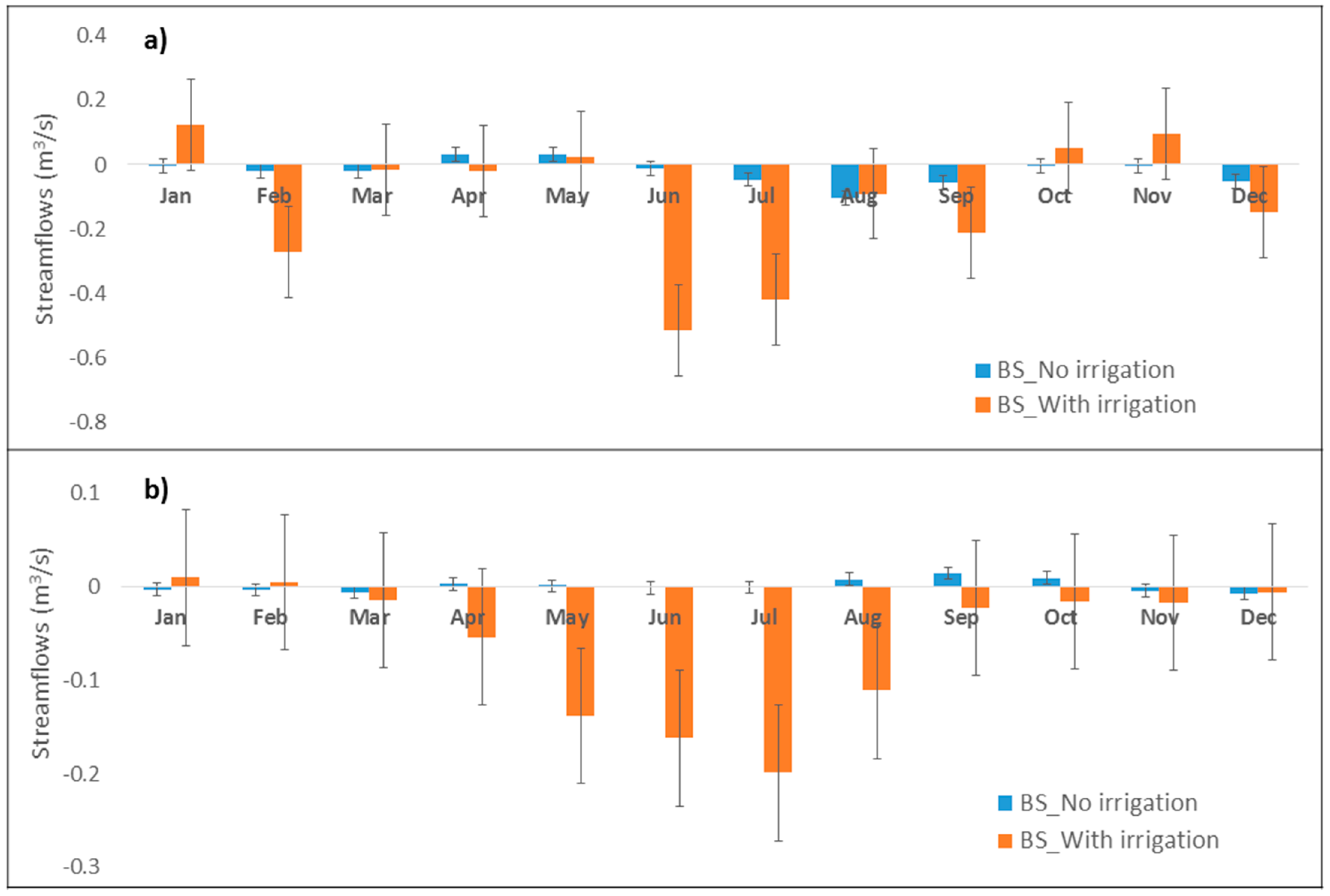
3.4. Effect of Irrigation Farm Dams

The agricultural sector of South Australia depends heavily on irrigation water from local catchments which includes the source from the surface runoff captured in farm dams [11]. Water from farm dams are stored mainly for irrigation. Thus, irrigated farm dams are expected to have important effects on the catchment hydrology as they affect the volume and movement of runoff [11,12]. A scenario analysis with and without farm dams revealed that the purpose of farm dams rather than the number of farm dams within a catchment area affected streamflow. The U-test for Below Holland Creek and Sixth Creek catchments indicated a clear difference in the streamflows between the scenarios with and without farm dams’ presence even though their areas in the catchments are significantly lower compared to the Kersbrook catchment (

Table 5. Statistical analysis of scenarios for stream flows with and without farm dams.

	Kersbrook	Sixth Creek	Below Holland Creek
Mann-Whitney (U-Test)
p-value	0.61	1.03 × 10−4	<2.2 × 10−16
Sensitivity	No	Yes	Yes
Catchment characteristics
Farm dams area (km2)	0.39 (1.74%) a	0.17 (0.39%) a	2.90 (1.29%) a
Horticulture-viticulture area (km2)	0.75 (3%) a	7.13 (17%) a	17.69 (8%) a
- Orchards	0.72	5.06	3.86
- Vegetables	-	0.97	0.45
- Vineyards	0.03	1.10	13.39

Notes: ^a Values in the parenthesis indicate the relative percent of area compared to the catchment area.

). These two catchments are characterized with intensive irrigation for horticultural land uses. In contrast, the presence of large areas of farm dams in the Kersbrook catchment with a limited area of horticulture and with restricted to no extraction for pasture irrigation and animal stock during the period of study [5] indicated low effects on streamflows. This further confirms that the drought condition of Kersbrook streamflow might be more associated with the catchment natural characteristics rather than with the effects of farm dams.

This pattern was further addressed when comparing the scenarios of farm dams’ effect in association with irrigation through the scenarios with farm dams not used for irrigation and with farm dams used for irrigation. This test was performed for the two catchments, i.e., Sixth Creek and Below Holland Creek which indicated a significant difference between cases with and without farm dams. The results showed that the scenario of no irrigation practices, although with farm dams’ presence, did not vary greatly in comparison with the scenario of removing farm dams (magnitude of change <0.1 m³/s). However, the scenario with irrigation application extracted from farm dams (BS_With irrigation) showed a significant change in the streamflows’ pattern in comparison to the scenario of no irrigation from farm dams (Figure 5). This indicated that the irrigation practices rather than the source of irrigation is the reason for the effect on streamflows.

Further analysis of the scenario with irrigation in comparison to other scenarios showed that a larger relative decline in streamflows was evident in the catchment with a more intensive irrigation practice. This was the case of Sixth Creek which had an irrigation rate for orchard land use of 5.09 ML/ha in comparison to Below Holland Creek which had a lower rate of irrigation for vineyards of 1.26 ML/ha. At monthly time steps, the most evident effect of irrigation farm dams on the decrease of the peak streamflows occurred in the rainy months of June and July. Overall, the models suggest that approximately 13.1% and 22.0% of water have been annually diverted from the natural streamflow of Below Holland Creek and Sixth Creek for irrigation purposes. These results are comparable with the outputs from the study of Heneker [11] which was the sole publication so far focused on modelling the hydrology of the study area. It was predicted by Heneker [11] that the rate of water being captured from farm dams might increase up to 19.0% to 26.0% in the following years which were predicted as drier years. Comparing the outputs from the scenarios, the lower rate of the flow decline in our study indicates that the restriction on water use might be an efficient solution to help protect the streams during periods of drought.

Although the amount of water captured from irrigation farm dams during rainy periods was significant in quantity, it did not decrease the streamflow to the dry level. In the case of Below Holland Creek catchment, the presence of irrigation farm dams in dry months (especially in January) even suggested a slight increase in the flow level (Figure 5). This might be an effect of irrigated water on fields during a period of no rain. Meanwhile at Sixth Creek catchment, the effect on streamflow drought was not evident as the creek has a stable flow level all the year. A similar finding was reported in a nearby catchment of the Eastern Mount Lofty Ranges (South Australia) which stated that additional irrigation might provide appreciable benefits to the downstream area, particularly during periods of low flows including January [15]. Clarifying this effect would benefit the planning of local managers in sustaining the local environmental flow. The accuracy of simulation results by these models can be improved by collecting data on irrigation at the catchment scale more frequently and increasing the number of streamflow gauging stations within the study area.

4. Conclusions

This study tested the effects of forest cover and irrigation farm dams on the streamflows of the three water-limited catchments in South Australia by means of the process-based model SWAT. The results have shown that:

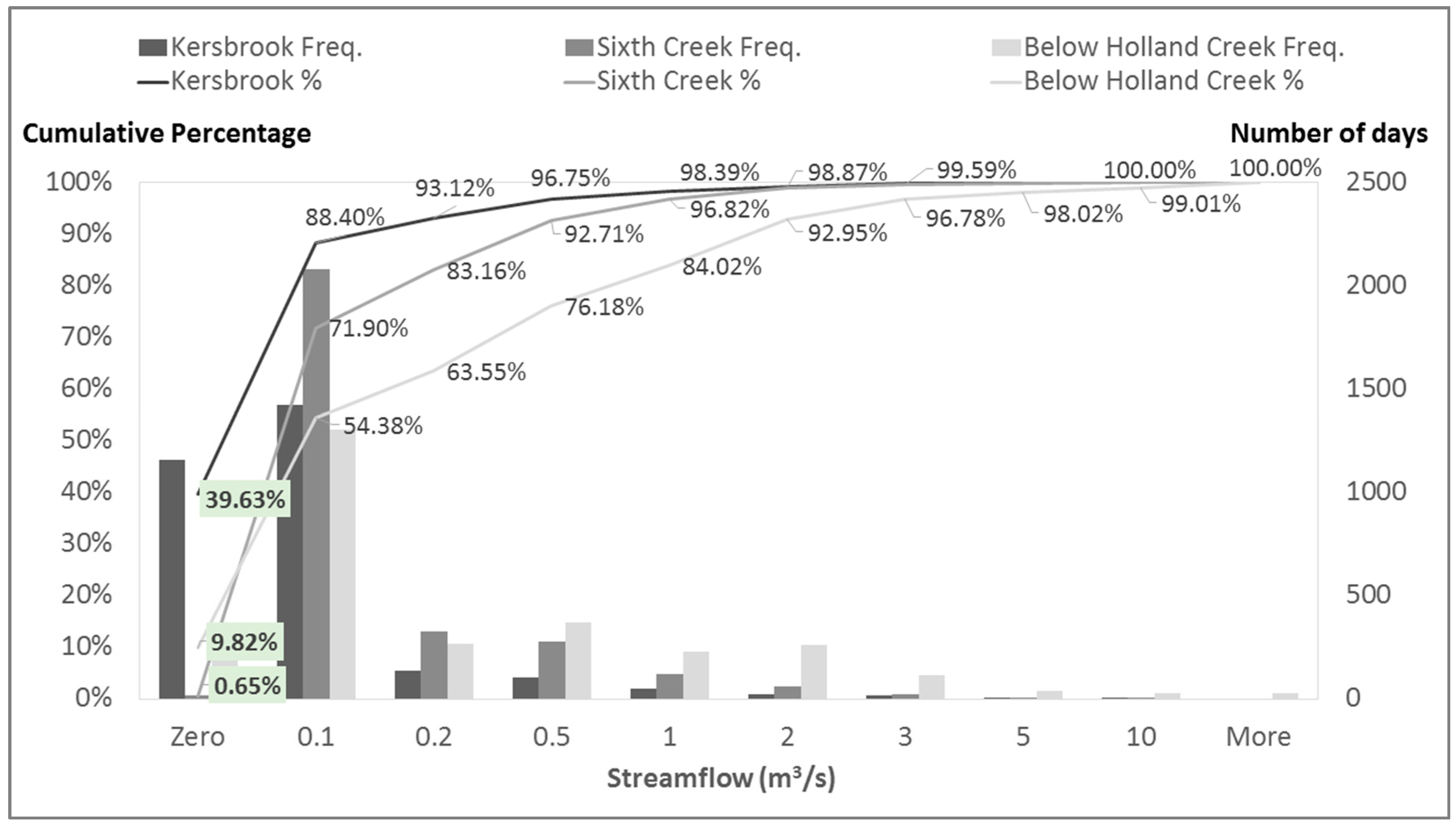
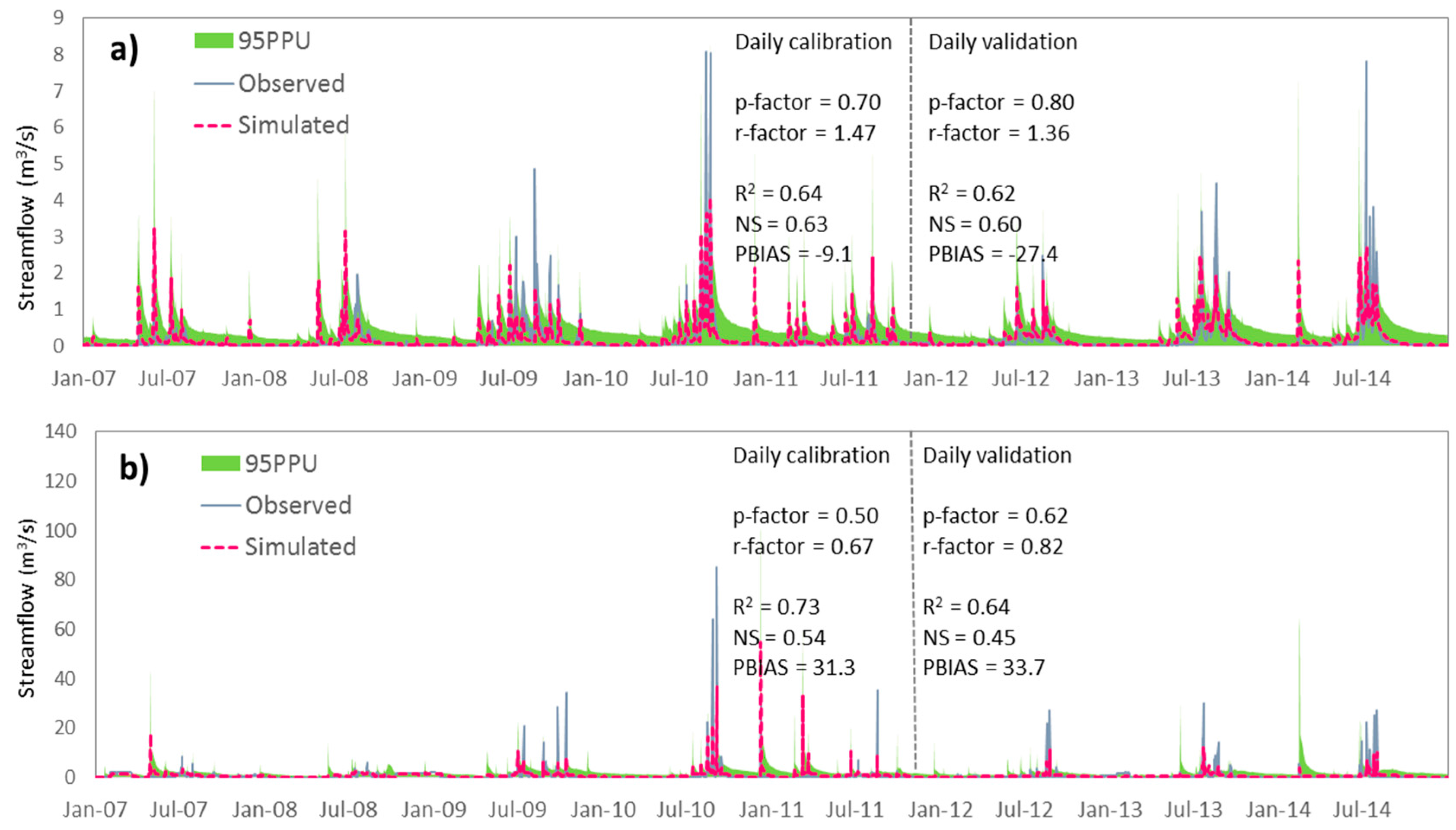
• The auto-calibration using NS as an objective function performed satisfactorily for catchments dominated by low flows (0.1 m³/s). Calibration statistics and uncertainty values met the criteria better when irrigation practices were properly characterized, both spatially and temporally, in the model.
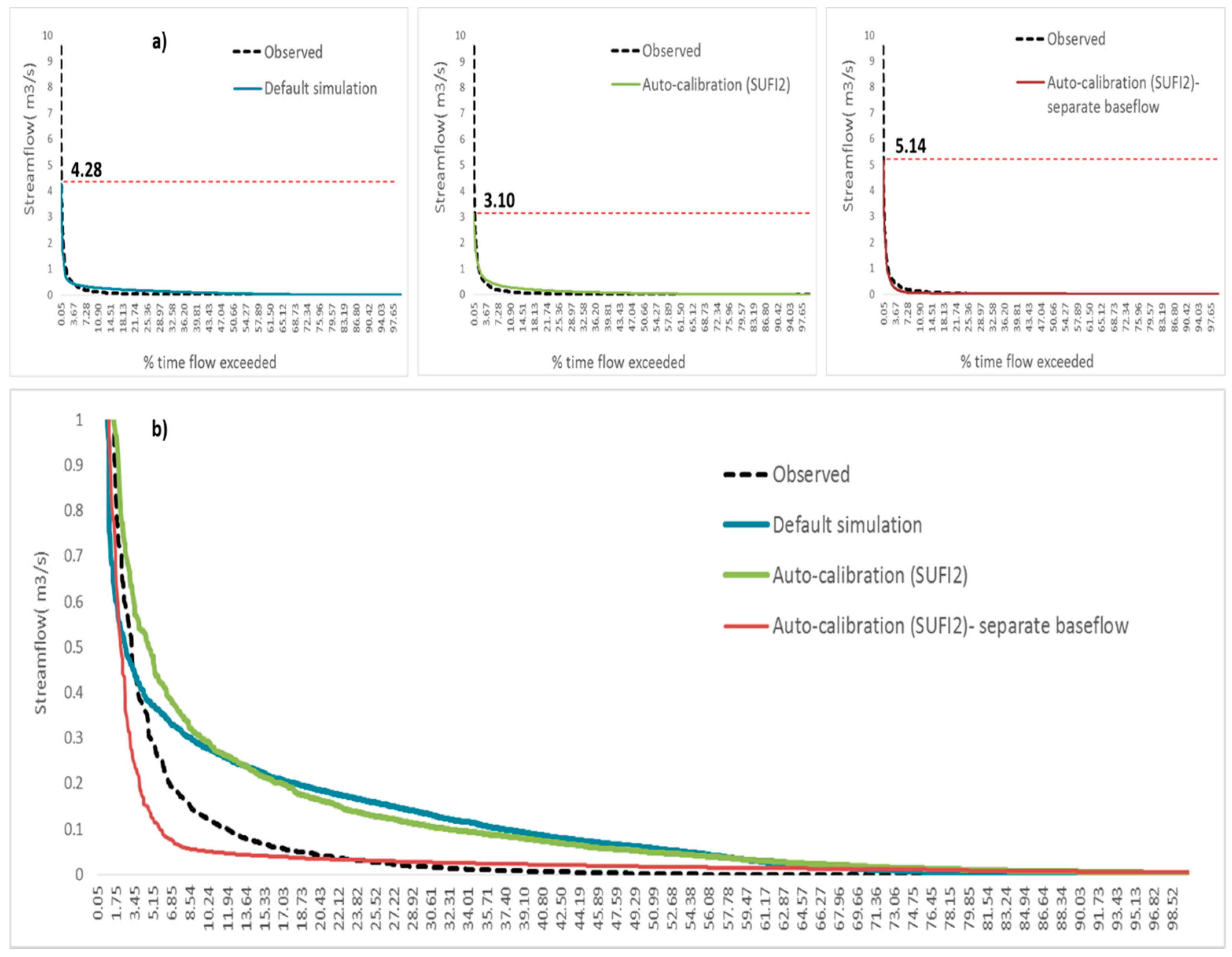
• The daily calibration improved significantly when the BFS method embedded in the NS analysis was applied for catchments dominated by zero flow.
• The projected extension of forest cover leads to a decrease in the simulated surface flow and water yield and an increase in the simulated ET and base-flow, while additional proportion of pasture caused the contrary pattern in water balance components.
• A scenario analysis indicated that the purpose of farm dams determined their effect on streamflows rather than the number of farm dams. Catchments with intensive irrigation by orchards and vineyards experienced more severe declines in streamflow during irrigation intensive seasons than catchments dominated by pastures.
• With water resources in the study area having recently been “prescribed” and extraction allocations being set, as well as extraction restrictions being applied during drought periods, modelling during the study time period suggested that effects of water extraction from farm dams had not significantly threatened natural streamflow conditions during those times. The model highlighted the importance of considering the effects of irrigation on the hydrology conditions of water limited catchments. The outputs from this study suggested a necessity to further investigate the effects of farm dams on the catchment hydrological dynamics apart from their roles solely as irrigation sources for the adaptive management of catchments.

The successful application of SWAT in this study provides a supplementary modelling tool for the more complex hydrological studies in comparison to the on-going developed Source model for Australian catchments. Successful hydrologic simulation in this study is a prerequisite for the further research with a focus on simulations of nutrient and pathogen loads within the integrated catchment. Future work will focus on the integration of the three catchments and adjacent drinking water reservoirs into comprehensive catchment models.

References

1. Van Otrop, F.F.; Vervoort, R.W.; Heller, G.Z.; Stasinopoulos, D.M.; Rigby, R.A. Long-range forecasting of intermittent streamflow. Hydrol. Earth Syst. Sci. 2011, 15, 3343–3354. [Google Scholar] [CrossRef] [Green Version]
2. Saha, P.P.; Zeleke, K. Rainfall-Runoff Modelling for Sustainable Water Resources Management: SWAT Model Review in Australia. In Sustainability of Integrated Water Resources Management. Water Governance, Climate and Ecohydrology (eBook); Setegn, S.G., Donoso, M.C., Eds.; Springer International Publishing AG: Cham, Switzerland, 2015; pp. 563–578. [Google Scholar]
3. Majumdar, D.K. Irrigation Water Management: Principle and Practice, 2nd ed.; Prentice-Hall of India: Delhi, India, 2013; p. 572. [Google Scholar]
4. Brown, S.C.; Versace, V.L.; Lester, R.E.; Walter, M.T. Assessing the impact of drought and forestry on stream flows in south-eastern Australia using a physically based hydrological model. Environ. Earth Sci. 2015, 74, 6047–6063. [Google Scholar] [CrossRef]
5. Australian Bureau of Statistics (ABS). Available online: http://www.abs.gov.au/AUSSTATS/[email protected]/second+level+view?ReadForm&prodno=4618.0&viewtitle=Water%20Use%20on%20Australian%20Farms~2007-08~Previous~26/05/2009&&tabname=Past%20Future%20Issues&prodno=4618.0&issue=2007-08&num=&view=& (accessed on 1 October 2015).
6. Shrestha, M.K.; Recknagel, F.; Frizenschaf, J.; Meyer, W. Assessing SWAT models on single and multi-site calibration for the simulation of flow and nutrients loads in the semi-arid Onkaparinga catchment in South Australia. Agric. Water Manag. 2016, 175, 61–71. [Google Scholar] [CrossRef]
7. Ilman, M.A.; Gell, P.A. Sediments, Hydrology and Water Quality of the River Torrens: A Modern and Historical Perspectives: Three Projects for the River Torrens Water Catchment Management Board; Department of Geographical and Environmental Studies, University of Adelaide: Adelaide, Australia, 1998; pp. 10–53. [Google Scholar]
8. Smakhtin, V.U. Low Flow Hydrology: A Review. J. Hydrol. 2001, 240, 147–186. [Google Scholar] [CrossRef]
9. Rebbeck, M.; Dwyer, E.; Bartetzko, M.; Williams, A. A Guide to Climate Change and Adaptation in Agriculture in South Australia; South Australian Research and Development Institute, Primary Industries and Resources SA and Rural Solutions SA: Urrbrae, Australia, 2007; pp. 12–22. [Google Scholar]
10. Hawthorne, K. A Methodology for Estimating Regional Agricultural Water Use; Research Paper 4616.0.55.001; Australia Bureau of Statistics: Belconne, Australia, 2006. Available online: http://www.ausstats.abs.gov.au/ausstats/subscriber.nsf/0/0186AA6011A98B42CA2571EE001EE96E/$File/4616055001_sep%202006.pdf (accessed on 6 January 2017).
11. Heneker, T.M. Surface Water Assessment of the Upper River Torrens Catchment; Report DWLBC 2003/2004; The Department of Water, Land and Biodiversity Conservation: Adelaide, Autralia, 2003; pp. 35–105.
12. Tingey-Holyoak, J.L. Water sharing risk in agriculture: Perceptions of farm dam management accountability in Australia. Agric. Water Manag. 2014, 145, 123–133. [Google Scholar] [CrossRef]
13. Pushpalatha, R.; Perrin, C.; Moine, N.L.; Andreassian, V. A review of efficiency criteria suitable for evaluating low-flow simulations. J. Hydrol. 2011, 420–421, 171–182. [Google Scholar] [CrossRef]
14. Demirel, M.C.; Booij, M.J.; Hoekstra, A.Y. The skill of seasonal ensemble low-flow forecasts in the Moselle River for three different hydrological models. Hydrol. Earth Syst. Sci. 2015, 19, 275–291. [Google Scholar] [CrossRef]
15. Alcorn, M.R. Hydrological Modelling of the Eastern Mount Lofty Ranges: Demand and Low Flow Bypass Scenarios; Department for Water: Adelaide, Australia, 2011; pp. 2–42. ISBN 978-1-921923-02-9. [Google Scholar]
16. Fleming, N.K.; Cox, J.W.; He, Y.; Thomas, S. Source Catchment Hydrological Calibration in the Mount Lofty Ranges Using PEST Parameter Optimisation Tool; eWater CRC: Canberra, Autralia, 2012; pp. 10–21. ISBN 978-1-921543-63-0. [Google Scholar]
17. Alcorn, M.R. Hydrological Model of the Onkaparinga Catchment, South Australia: Calibration Report; DEWNR Technical Report 2015/02; Department of Environment, Water and Natural Resources: Adelaide, Australia, 2015; pp. 2–24. ISBN 978-1-922255-29-7. [Google Scholar]
18. Marston, F.; Argent, R.; Vertessy, R.; Cuddy, S.; Rahman, J. The Status of Catchment Modelling in Australia. Cooperative Research Centre for Catchment Hydrology; Technical Report 02/04; Monash University: Melbourne, Australia, 2002. [Google Scholar]
19. Arnold, J.G.; Srinivasan, R.; Muttiah, R.S.; Williams, J.R. Large area hydrologic modelling and assessment part I: Model development. J. Am. Water Resour. Assoc. 1998, 34, 73–89. [Google Scholar] [CrossRef]
20. Gassman, P.W.; Reyes, M.R.; Green, C.H.; Arnold, J.G. The Soil and Water Assessment Tool: Historical development, applications and future research directions. Trans. ASAE (Am. Soc. Agric. Eng.) 2007, 50, 1211–1250. [Google Scholar] [CrossRef]
21. Moriasi, D.N.; Arnold, J.; Van Liew, M.; Bingner, R.L.; Harmel, R.D.; Veith, T.L. Model evaluation guidelines for systematic quantification of accuracy in watershed simulations. Trans. ASAE (Am. Soc. Agric. Eng.) 2007, 50, 885–900. [Google Scholar]
22. Arnold, J.G.; Moriasi, D.N.; Gassman, P.W.; Abbaspour, K.C.; White, M.J.; Srinivasan, R.; Santhi, C.; Harmel, R.D.; van Griensven, A.; Van Liew, M.W.; et al. SWAT: Model use, calibration, validation. Trans. ASABE (Am. Soc. Agric. Eng.) 2012, 55, 1491–1508. [Google Scholar]
23. Abbaspour, K.C.; Rouholahnejad, E.; Vaghefi, S.; Srinivasan, R.; Yang, H.; Klove, B. A continental-scale hydrology and water quality model for Europe: Calibration and uncertainty of a high-resolution large scale SWAT model. J. Hydrol. 2015, 524, 733–752. [Google Scholar] [CrossRef]
24. Saha, P.P.; Zeleke, K.; Hafeez, M. Streamflow modelling in a fluctuant climate using SWAT: Yass River catchment in south eastern Australia. Environ. Earth Sci. 2014, 71, 5241–5254. [Google Scholar] [CrossRef]
25. Schuol, J.; Abbaspour, K.C.; Yang, H.; Srinivasan, R.; Zhender, A.J.B. Modeling blue and green water availability in Africa. Water Resour. Res. 2015, 44, 1–18. [Google Scholar] [CrossRef]
26. Pfannerstill, M.; Björn, G.; Fohrer, N. Smart Low Flow Signature Metrics for an Improved Overall Performance Evaluation of Hydrological Models. J. Hydrol. 2014, 510, 447–458. [Google Scholar] [CrossRef]
27. Krause, P.; Boyle, D.P.; Bäse, F. Comparison of different efficiency criteria for hydrological model assessment. Adv. Geosci. 2005, 5, 89–97. [Google Scholar] [CrossRef]
28. Muleta, M.K. Improving Model Performance Using Season-based Evaluation. J. Hydrol. Eng. 2012, 17, 191–200. [Google Scholar] [CrossRef]
29. Kim, H.S.; Lee, S. Assessment of a seasonal calibration technique using multiple objectives in rainfall-runoff analysis. Hydrol. Process. 2014, 28, 2159–2173. [Google Scholar] [CrossRef]
30. Zang, D.; Chen, X.; Yao, H.; Lin, B. Improved calibration scheme of SWAT by separating wet and dry seasons. Ecol. Model. 2015, 301, 54–61. [Google Scholar] [CrossRef]
31. Brindal, M.; Stringer, R. Water Scarcity and Urban Forests: Science and Public Policy Lessons from a Decade of Drought in Adelaide, Australia. Arboric. Urban For. 2013, 39, 102–108. [Google Scholar]
32. Bureau of Meteorology (BOM). Available online: http://www.bom.gov.au/climate/updates/articles/a010-southern-rainfall-decline.shtml (accessed on 2 January 2016).
33. Australian Soil Resource Information System (ASRIS). Available online: http://www.asris.csiro.au/mapping/viewer.htm (accessed on 1 March 2015).
34. Scientific Information for Land Owners (SILO). Available online: http://www.longpaddock.qld.gov.au/silo/ppd/index.php (accessed on 1 February 2015).
35. Winchell, M.; Srinivasan, R.; Di Luzio, M.; Arnold, J. Arc SWAT Interface for SWAT2012 User’s Guide; Texas AgriLife Research and United States Department of Agriculture: Temple, TX, USA, 2013.
36. Neitsch, S.L.; Arnold, J.G.; Kinir, J.R.; Wiliams, J.R. Soil and Water Assessment Tool: Theoretical Documentation 2009; Technical Report No. 406; Texas Water Resources Institute-Texas A&M University: College Station, TX, USA, 2011; pp. 29–180. [Google Scholar]
37. Soil Conservation Service (SCS). Section 4-Hydrology. In SCS National Engineering Handbook; USDA: Washington, DC, USA, 1972. [Google Scholar]
38. Hargreaves, G.H.; Samani, Z.A. Reference crop evapotranspiration from temperature. Appl. Eng. Agric. 1985, 1, 96–99. [Google Scholar] [CrossRef]
39. Arnold, J.G.; Kiniry, J.R.; Srinivasan, R.; Wiliams, J.R.; Haney, E.B.; Neitsch, S.L. Soil and Water Assessment Tool: Input/Output Documentation; Technical Report; Texas Water Resources, Institute-Texas A&M University: College Station, TX, USA, 2012; Volume 439, pp. 2–620. [Google Scholar]
40. Data.SA (South Australian Government Data Directory). Available online: http://data.sa.gov.au/data/dataset/cc790713-4cf0-4bd4-bca8-f195d8e202b7 (accessed on 1 November 2015).
41. Abbaspour, K.C. SWAT-CUP: SWAT Calibration and Uncertainty Programs—A User Manual; Eawag: Dübendorf, Switzerland, 2015; pp. 16–70. [Google Scholar]
42. Abbaspour, K.C.; Yang, J.; Maximov, I.; Siber, R.; Boger, K.; Mieletner, J.; Zobrist, J.; Srinivasan, R. Modelling hydrology and water quality in the pre-alpine/alpine Thur watershed using SWAT. J. Hydrol. 2007, 333, 413–430. [Google Scholar] [CrossRef]
43. Githui, F.; Thayalakumaran, T.; Selle, B. Estimating irrigation inputs for distributed hydrological modelling: A case study from an irrigated catchment in southeast Australia. Hydrol. Process. 2015, 30, 1824–1835. [Google Scholar] [CrossRef]
44. Tuppad, P.; Douglas-Mankin, K.R.; Lee, T.; Srinivasan, R.; Arnold, J.G. Soil and Water Assessment Tool (SWAT) hydrologic/water quality model: Extended capability and wider adoption. Trans. ASABE 2011, 54, 1677–1684. [Google Scholar] [CrossRef]
45. Hulme, K.A. Eucalyptus Camaldulensis (River Red Gum). Biogeochemistry: An Innovative Tool for Mineral Exploration in the Curnamona Province and Adjacent Regions. Ph.D. Thesis, School of Earth and Environmental Sciences, University of Adelaide, Adelaide, Australia, 2008. [Google Scholar]
Figure 1. The study area: (a) Locations of gauging stations; (b) Land uses map.
Water 09 00033 g001
Figure 2. Frequency distribution of streamflows in the Kersbrook, Sixth Creek, and Below Holland Creek catchments.
Water 09 00033 g002
Figure 3. Model calibration and validation with daily time steps for (a) Sixth Creek and (b) Below Holland Creek.
Water 09 00033 g003
Figure 4. Daily observed and simulated flow duration curves of the Kersbrook catchment. (a) Highlight peak flow parts. Bold numbers indicate maximum flows; (b) Highlight low flow parts.
Water 09 00033 g004
Figure 5. Changes in streamflows at Below Holland Creek (a) and Sixth Creek (b) for the scenarios with farm dams not used for irrigation (BS_No irrigation) and used for irrigation (BS_With irrigation). Error bars show one standard deviation.
Water 09 00033 g005