Article

Determination of Growth Stage-Specific Crop Coefficients (Kc) of Sunflowers (Helianthus annuus L.) under Salt Stress

1
State Key Laboratory of Water Resources and Hydropower Engineering Science, Wuhan University, Wuhan 430072, China
2
Crop Science Group, Institute of Crop Science and Resource Conservation (INRES), University of Bonn, Katzenburgweg 5, D-53115 Bonn, Germany
3
State Key Laboratory of Hydrology-Water Resources and Hydraulic Engineering, Hohai University, Nanjing 210098, China
4
Department of Hydrology and Water Resources, Hohai University, Nanjing 210098, China
*
Author to whom correspondence should be addressed.
Water 2017, 9(3), 215; https://doi.org/10.3390/w9030215
Submission received: 16 January 2017 / Accepted: 9 March 2017 / Published: 13 March 2017

Abstract

:
Crop coefficients (Kc) are important for the development of irrigation schedules, but few studies on Kc focus on saline soils. To propose the growth-stage-specific Kc values for sunflowers in saline soils, a two-year micro-plot experiment was conducted in Yichang Experimental Station, Hetao Irrigation District. Four salinity levels including non-salinized (ECe = 3.4–4.1 dS·m–1), low (ECe = 5.5–8.2 dS·m–1), moderate (ECe = 12.1–14.5 dS·m–1), and high (ECe = 18.3–18.5 dS·m–1) levels were arranged in 12 micro-plots. Based on the soil moisture observations, Vensim software was used to establish and develop a physically-based water flow in the soil-plant system (WFSP) model. Observations in 2012 were used to calibrate the WFSP model and acceptable accuracy was obtained, especially for soil moisture simulation below 5 cm (R2 > 0.6). The locally-based Kc values (LKc) of sunflowers in saline soils were presented according to the WFSP calibration results. To be specific, LKc for initial stages (Kc1) could be expressed as a function of soil salinity (R2 = 0.86), while R2 of LKc for rapid growth (Kc2), middle (Kc3), and mature (Kc4) stages were 0.659, 1.156, and 0.324, respectively. The proposed LKc values were also evaluated by observations in 2013 and the R2 for initial, rapid growth, middle, and mature stages were 0.66, 0.68, 0.56 and 0.58, respectively. It is expected that the LKc would be of great value in irrigation management and provide precise water application values for salt-affected regions.

1. Introduction

Sunflower (Helianthus annuus L.) is one of the four most important oil crops in the world [1]. Based on data from the National Sunflower Association, more than 25 million hectares of global croplands are planted in sunflowers. The Hetao Irrigation District, which is located in northern China, is the largest sunflower-growing region in China, and sunflower seeds are the main source of income for local farmers [2]. However, due to high rates of evaporation and low levels of precipitation, the significance of irrigation in attaining and sustaining optimum productivity of major crops in the Hetao Irrigation District or other regions with similar climate conditions is important and has been documented [3,4]. Demir et al. [1] reported that the seed and oil yield of oil sunflowers increased by 82.9% and 85.4% with irrigation as compared to the treatment without irrigation at three growth stages of sunflowers in Turkey; Ertek and Kara [5] also conducted a series of deficit irrigation experiments, and concluded that maize fresh ear yield was affected by water stress. Furthermore, between yield and water use, a positive linear relationship has been recognized by various researchers [6,7,8,9,10]. However, because of the limited knowledge of crop water use in this region, flood irrigation without scheduling is still the main irrigation practice, which is not only a non-efficient use of water resources but also has the possibility for increasing the risk of groundwater contamination because a large number of solutes could be leached below the root zone using this irrigation practice [11]. Therefore, it is necessary to determine an efficient and representative irrigation scheduler to improve the crop productivity and water resource management for the region.
Crop evapotranspiration (ETc), which represents the combined processes of water loss through evaporation from soil surface and transpiration from crop surface, has a potential advantage to attain proper irrigation scheduling [12,13]. Although there are few traditional technologies (e.g., weighting lysimeters, sap-flow sensors) that can assist scientists with determining ETc [14], it is still laborious, time-consuming and costly to apply these technologies in large regions [15]. As recommended by Food and Agricultural Organization (FAO) [16], the approach of the crop coefficient (Kc) is widely used to estimate crop water use and to schedule irrigations. The concept of Kc was introduced by Jensen [17] and further developed by the other researchers [16,18,19]. Generally speaking, Kc is defined as the ratio between ETc and reference evapotranspiration (ET0) which is based on the evapotranspiration (ET) rate from a well-water (not limiting) reference surface. As discussed and summarized in the FAO document, the single crop coefficient approach is used for most applications related to irrigation planning, design, and management due to its simplicity. Values of Kc for most agricultural crops increase from a minimal value at planting to a maximum Kc value near full canopy cover or pollination. FAO provides details on the development and use of generalized Kc values for different crops in different regions of the world [16]. However, few methods available to attain crop coefficients for site-specific values have been determined experimentally for different growth stages of sunflowers. What data is available is considerably different from that listed in the FAO-56 paper [20]. Meanwhile, approximately 70% of the cultivated land in the Hetao Irrigation District is contaminated by soil salinity, which has been proven to be a vital factor affecting crop growth [3,21]. Based on our previous works, soil salinity affects sunflower growth elements such as the photosynthesis [22] and dry matter formation [23], which indicates that there may be a direct relationship between soil salinity and Kc. However, as far as we know, almost no published studies focus on this correlation. Therefore, it is important to determine local-based Kc values for more precise crop ETc estimation, especially for crops growing in saline soils. However the traditional method for estimating Kc is usually via weighting lysimeters [24], which is both costly and time consuming. Due to the lack of research-based information on sunflower water use in saline soils and the inconvenience of directly experimental Kc determination, the objectives of this study were to (1) construct a physically-based model to determine local growth-stage-specific Kc values for sunflowers in different levels of saline soils, and (2) to ascertain the relationship between Kc values and soil salinity (Kc-S). Also, evaluations for both model performance and the Kc-S relationship were performed based on field experiments.

2. Materials and Methods

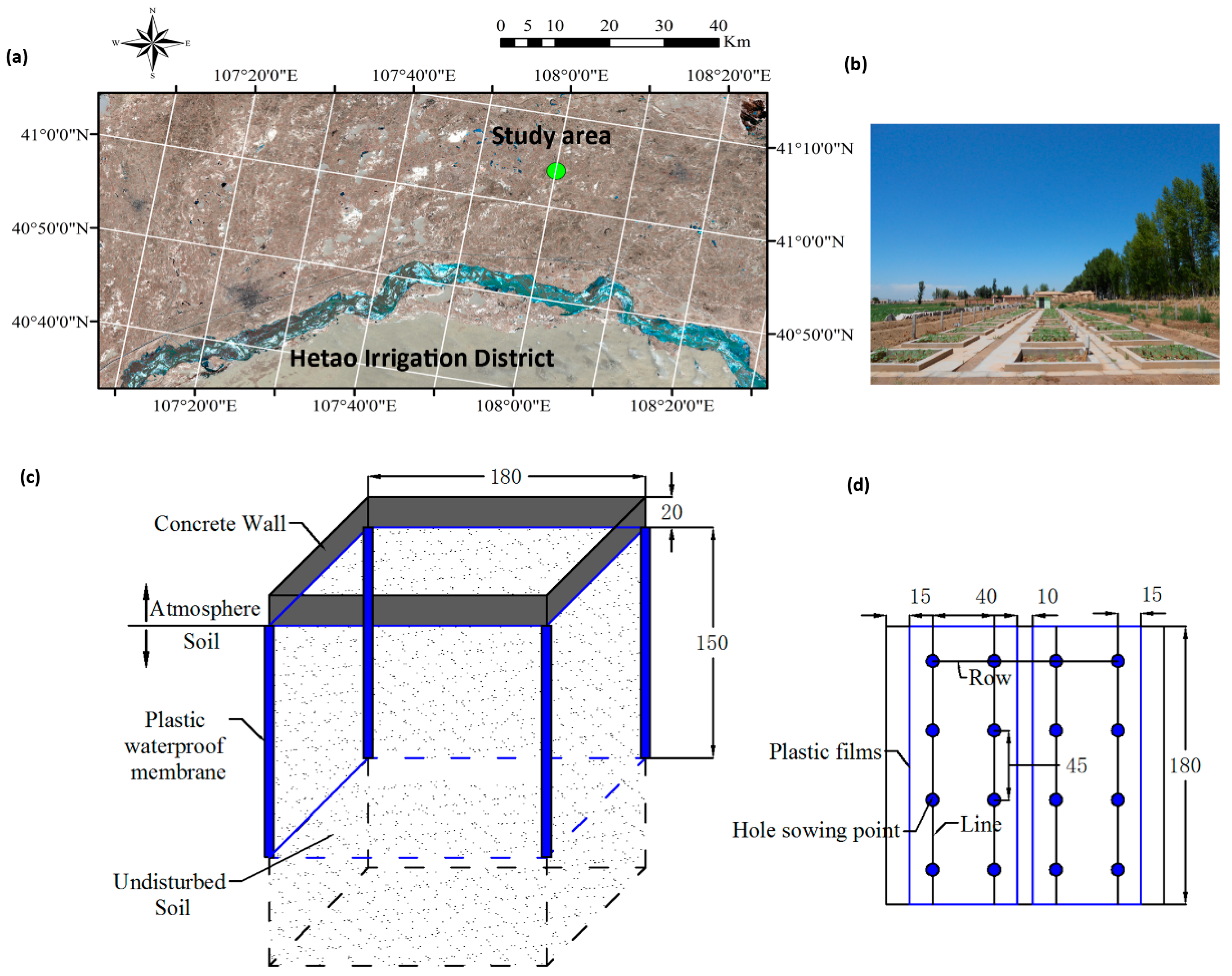
2.1. Study Site Characteristics and Field Experiment Design

This experiment was conducted at the Yichang Experimental Station in the Hetao Irrigation District (40°19′ to 41°18′ N, 106°20′ to 109°19′ E), Inner Mongolia, China (Figure 1a). The Hetao Irrigation District has the largest gravity irrigation area (~1.05 × 10⁶ ha) in China and is representative of the continental climate. The mean annual precipitation and mean annual potential evapotranspiration are approximately 176 mm and 2056 mm, respectively, and 63%–70% of precipitation is from June to August [4]. Micro-plot experiments were conducted on sunflowers (Helianthus) for two years, in 2012 and 2013. Each micro-plot covered an area of 1.8 m × 1.8 m and was surrounded by an impermeable plastic barrier to a depth of 1.5 m to prevent lateral drainage (Figure 1b,c). Salt crusts on the surface of saline bare soils were collected and used to modify salinity from the 0–20 cm depth of the micro-plots. Saturated electrical conductivity (ECe) was used to indicate soil salinity levels. Four different salinity levels were established, including non-salinized (ECe = 3.4–4.1 dS·m–1), low (ECe = 5.5–8.2 dS·m–1), moderate (ECe = 12.1–14.5 dS·m–1), and high (ECe = 18.3–18.5 dS·m–1), respectively. Sunflowers (cv. LD5009) were planted on 7 June 2012 and 4 June 2013 in a grid of four rows (0.45 m × 0.4 m spacing) within each subplot (Figure 1d); the plant density was 4.94 plants m−2, and soil was covered by plastic films in order to decrease soil evaporation. Plants were harvested on 24 September 2012 and 16 September 2013. More details for the micro-plot experiments can be found in [21]. Sunflower growth periods were divided into four stages including initial stage, rapid growth stage, middle stage, and mature stage [25]. Soil samples at different depths were taken at sowing stage and four times for each subsequent growth stage. Soil samples were taken at depths of 0–5, 5–10, 10–20, 20–40, 40–60, 60–80, and 80–100 cm on 10 June, 13 July, 2 August, 9 August, and 24 September in 2012 and at depths of 0–10, 10–20, 20–30, 30–40, 40–60, 60–80, 80–100 cm on 30 May, 10 July, 24 July, 14 August, and 16 September in 2013, respectively. After sampling, soil moisture was determined using the oven-dry method. Soil texture was analyzed using the pipette method [26,27] and the bulk density was measured by the cutting-ring method [27,28] (Table 1).

2.2. Model Descriptions

System Dynamics (SD) was firstly proposed by Forrester [29] and widely applied to analyze the change of a modeling system based on the linkage and response mechanism among models, which can represent complex systems and analyze their dynamic behavior [30]. Vensim software (http://vensim.com/) has been shown to be an adequate tool to depict system dynamics [31,32,33]. Vensim™, the Ventana® Simulation Environment, is an interactive software environment that allows the development, exploration, analysis and optimization of simulation models. It was created to increase the capabilities and productivity of skilled modelers and has the functionality that improves the quality and understanding of models [34]. In this study, Vensim software was used to establish a physically-based model to consider the water flow in the soil–plant system (WFSP model). Vensim is designed to simultaneously solve a series of material held within a stock and its depletion or replenishment by flow into and out of the stock [35,36], and its open version Vensim PLE is freely available to the academic community for use in education and research. Here, stocks represent the mass of water within a given soil layer; while the flows represent the fluxes of water among stocks, model runs were conducted using a one-day time step, with state variables at each interval. All storage terms were given in millimeters; also, flow terms were given in millimeters per day. More details about this model, including the equations used to calculate the stocks and the flows are shown in following sections.

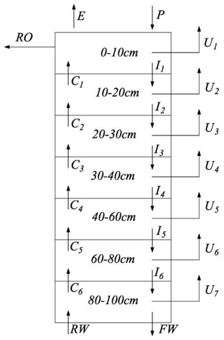
2.2.1. Basic Principles

Figure 2 indicates the water movement in the root zone of sunflowers for our model. Based on our soil sampling design, we considered a 100-cm depth soil profile and divided it into seven layers (0–5, 5–10, 10–20, 20–40, 40–60, 60–80, and 80–100 cm, for 2012 and for 2013, 0–10, 10–20, 20–30, 30–40, 40–60, 60–80, and 80–100 cm).
For the layer 1, layers 2–6, and layer 7, we can describe the water movement by Equations (1)–(3) respectively.
Δ S 1 = S 1 , t S 1 , t 1 = P + C 1 RO U 1 I 1 E
Δ S i = S i , t S i , t 1 = C i + I i 1 C i 1 U i I i
Δ S 7 = S 7 , t S 7 , t 1 = I + RW FW U 7 C 6
where S is soil water storage within every soil layer (subscript i represents a soil layer) (mm), P is precipitation (mm); C is the capillary water movement into the soil layer (mm); I is the seepage movement out of the soil layer (mm); E is soil evaporation (mm); and U is root water uptake from the soil layer (mm). RO is the surface runoff (mm), and because of the scarce precipitation in Hetao District, RO equals zero; RW is the groundwater recharge (mm); FW is the water flow out of the whole root zone (mm) and ΔS is the change of water storage for the specific soil layer (mm) during the time interval. Subscript t indicates the current moment (day) and t − 1 indicates the last moment (day). Subscript i indicates the layer number (from 2 to 6).

2.2.2. Infiltration

Infiltration is described based on Kostiakov [37] model (Equation (4)).
i t = i 1 t p
where it is the infiltration rate at time t (h) and expressed using the infiltration depth at unit time (cm·h−1); i1 is the infiltration rate for the first unit time; p is the empirical index which ranges from 0.3 to 0.8 and is based on the soil properties and moisture, and p is initially determined as 0.5 in this study.
Unsaturated hydraulic conductivity (K, mm·d−1) is calculated by van Genuchten [38] and van Genuchten and Nielsen [39] (Equations (5) and (6)).
K = K s ( θ θ r θ s θ r ) 0.5 { 1 [ 1 ( θ θ r θ s θ r ) 1 m ] m } 2
m = 1 1 n
where Ks is the saturated hydraulic conductivity (mm·d−1); θ is the soil moisture (cm3·cm−3); θr and θs are the residual and saturated soil moistures (cm3·cm−3) respectively; and m, n are dimensionless empirical parameters. Parameters for Equation (5) were predicted using the Rosetta module [40] based on soil particle size and bulk density (Table 2).
If soil moisture in the upper layer (θ) is larger than θs, I (Figure 2, Equations (1)–(3)) from the upper layer to the lower layer is equal to θ − θs; if θ ranges from θr to θs, I is equal to K; otherwise, I = 0.

2.2.3. Groundwater Recharge

Groundwater table (GWT) depths were obtained according to the local water resources bulletin and Liang et al. [41]. More exactly, the GWT depths of study area ranged from 1.14 m (November) to 2.59 m (March) and averaged at 1.82 m in 2012. In 2013 the lowest, deepest and average GWTs were 1.45 m (November), 2.33 m (March) and 1.91 m, respectively.
Groundwater recharge (RW) was calculated based on empirical formula proposed by Li [42] and Du et al. [25].
W g W c = 0.54742 H + 1.66494
where Wg is available groundwater (mm); Wc is the crop water requirement (mm); and H is the GWT (m).
Distribution of RW in the soil profile was calculated based on Feng and Liu [43] and Chen et al. [44], which was also to be used in the CERES-Wheat model (Equation (8)).
w i + 1 t = W g ( θ i + 1 t θ w i + 1 ) h i + 1 ( θ i t θ w i ) h i 0.5 ( h i + h i + 1 )
where w i + 1 t is water flux moving upward from layer i + 1 to layer i by capillarity at time t (mm); θ i + 1 t , θ i t , θ w i + 1 , and θ w i are soil moisture and wilting point of layer i + 1 and layer i at time t (cm3·cm−3); hi and hi+1 are the thicknesses of layer i + 1 and layer i (cm).

2.2.4. Root Distribution

Root distribution was determined according to the researches of Gale and Grigal [45] and Jackson et al. [46] (Equation (9)).
Y ( z ) = 1 β z
where Y(z) is the accumulated root percentage with soil depth (%) and z is the soil depth (100 cm) calculated from surface and the positive direction is downward (cm). β is an empirical parameter affected by plant types, soil and climate conditions. Jackson et al. [46] indicated that β ranges from 0.913 to 0.978; in our study, β was defined as 0.95.

2.2.5. Root Water Uptake

The Feddes et al. [47] model was used to determine root water uptake (RWU) (Equation (10)).
RWU = α ( h ) 0 L α ( h ) dz T p
where RWU is the root water uptake rate (mm·d−1); L is the root depth (100 cm); Tp is the potential transpiration rate (mm·d−1); z is the coordinate axis and positive downward (cm); and α(h) is the function about the soil water potential (SWP) (Equation (11)).
α ( h ) = { h 1 h , h h 1 1 , h 2 h < h 1 h h 3 h 2 h 3 , h 3 h < h 2 0 , h < h 3 }
In Equation (11), h is the soil water potential (cm). h1, h2, and h3 are three threshold values of soil water potential. To be specific, if soil is very wet and has poor ventilation when SWP is higher than h1, then RWU decreases with SWP. h2 is the SWP when plant suffers from water stress and h3 is the SWP at the wilting point.
Due to the SWP measurements being costly and time consuming, Feddes et al. [48] also proposed that SWP could be replaced by soil moisture (Equation (12)).
f ( θ ) = { 0 , θ θ wilt θ θ wilt θ stress θ wilt , θ wilt < θ < θ stress 1 , θ > θ stress
In Equation (12), θ is soil moisture (cm3·cm−3); θwilt is the wilting point expressed by moisture (cm3·cm−3); θstress is the soil moisture when plant is under water stress (cm3·cm−3). The details about parameters in Equation (12) are shown in Table 3. More exactly, the ranges of parameters in Equations (10)–(12) were determined according to previous studies [32,49] and the exact parameters value were calibrated based on the soil moisture observations in non-saline treatments using a trial-and-error method, which is a fundamental method of problem solving, characterized by repeated, varied attempts until acceptance of results [50].
By considering the root distribution (Section 2.2.4) together, the rate of RWU can be expressed as Equation (13).
RWU = T p f ( θ ) Y ( z )

2.2.6. Evapotranspiration and Crop Coefficients (Kc)

Reference evapotranspiration (ET0) was calculated based on Penman–Monteith equations [16] (Equation (14)).
E T 0 = 0.408 Δ ( R n G ) + γ 900 T + 273 u 2 ( e s e a ) Δ + γ ( 1 + 0 . 34 u 2 )
where ET0 is the reference evapotranspiration (mm·d−1); Rn is net radiation at the crop surface (MJ·m−2·d−1); G is soil heat flux density (MJ·m−2·d−1); T is mean daily air temperature at 2-m height (°C); u2 is wind speed at 2 m height (m·s−1); es is saturation vapor pressure (kPa); ea is actual vapor pressure (kPa); es − ea is saturation vapor pressure deficit (kPa); Δ is slope vapor pressure curve (kPa·°C−1); and γ is psychrometric constant (kPa·°C−1).
Since sunflowers were sown below plastic films (reducing surface evaporation), the single crop coefficient (Kc) method was used to calculated the crop water requirement (ETc) (Equation (15)).
E T c = K c · E T 0 = E p + T p
In Equation (15), Ep and Tp are potential soil evaporation and potential transpiration, respectively (mm·d−1). Considering the plastic films that could reduce evaporation and regarding its coefficient as an adjustable parameter (values ranging from 0 to 0.5) [51], and through calibration we chose 0.1 for an appropriate value; thus Ep was determined as in Equation (16).
E p = 0.1 E T c
Then,
T p = K c · E T 0 E p
Sunflower growth periods were divided into four stages (noted as day after sowing (DAS)), initial stage (DAS: 1–36), rapid growth stage (DAS: 37–57), middle stage (DAS: 58–90), and mature stage (DAS: 90–109) according to the study of Du et al. [25] and Allen et al. [16]. Initial Kc values for each stage were 0.3, 0.75, 1.2, and 0.35, respectively [16].

2.2.7. Modeling Process

Soil water flow and water uptake by sunflowers were computed for a soil profile with 100-cm depth. The simulation period extended from the early June to late September, and corresponded to the growth period of sunflowers. First, soil moisture observations in 2012 were used to calibrate the Kc for each stage of sunflowers. In this step, only Kc values were modified and other parameters (e.g., Table 2 and Table 3) were not changed because we assumed that the effects of salinity on sunflower growth could be reflected by Kc. Then the local-based Kc values for sunflower growing in the saline soils involving a relationship between Kc of initial stage and soil salinity were proposed. After that, soil moisture observations in 2013 were used to evaluate the proposed local-based Kc values and the contrastive analysis between our Kc values against previously reported research results.

2.3. Statistical Analysis

The determination coefficient (R2, Equation (18)) and the root-mean-square error (RMSE, Equation (19)) were used to evaluate the model performance.
R 2 = [ i = 1 n ( Y i obs Y ¯ i obs ) ( Y i sim Y ¯ i sim ) i = 1 n ( Y i obs Y ¯ i obs ) 2 i = 1 n ( Y i sim Y ¯ i sim ) 2 ] 2
RMSE = i = 1 n ( Y i obs Y i sim ) 2 n
where Yiobs is the ith observed value, Yisim is the ith simulated value, and Y i obs ¯ and Y i sim ¯ are the means of the observed and simulated values, respectively.

3. Results

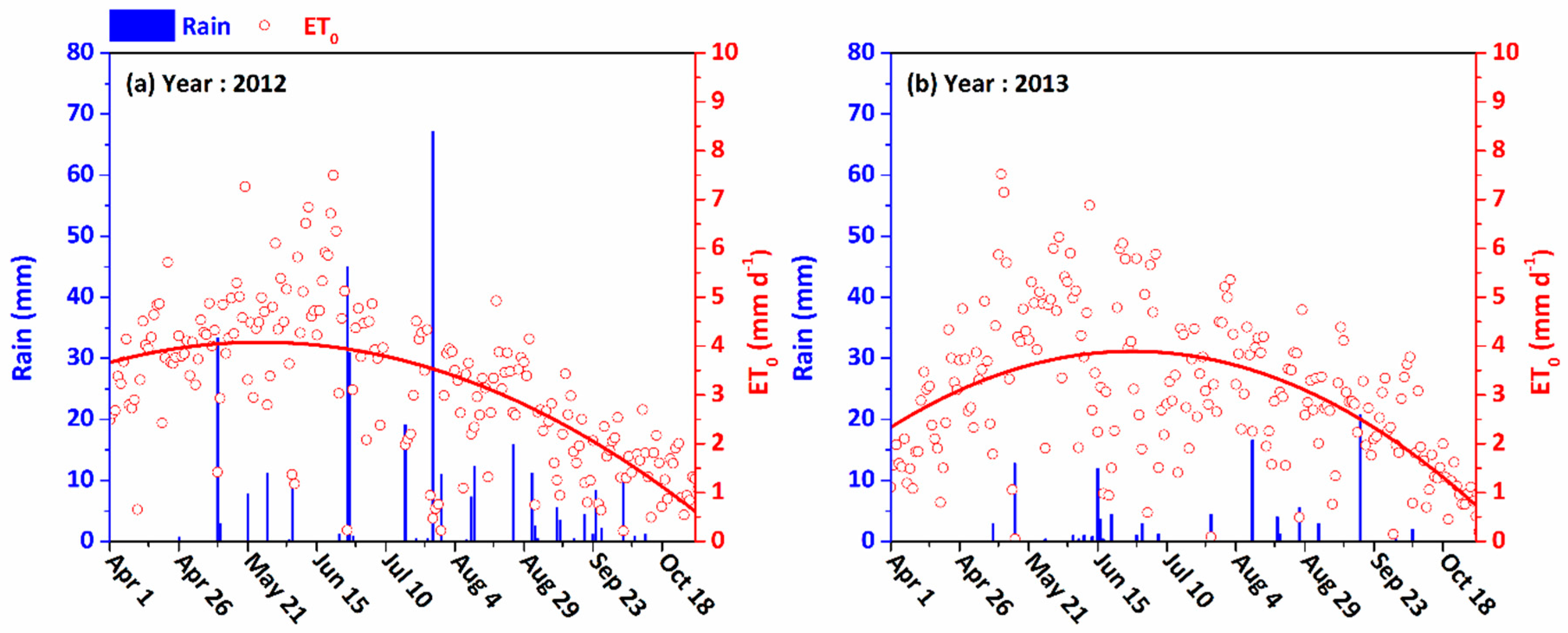
3.1. Meteorological Conditions

The daily precipitation measured by the field meteorological station of the experiment station from April to October in 2012 and 2013 varied from 0–67.2 mm·d−1 to 0–20.8 mm·d−1, respectively, with an accumulated precipitation of 254 mm for 2012 and 64.8 mm for 2013 (Figure 3), which indicated that the year 2012 was much wetter than 2013. Furthermore, the local water resources bulletin also confirmed that the 2012 was a wet year while 2013 was a drier one. Specifically, the total precipitation of 2012 in our experiment station is 400.6 mm (from April to October), which was about 127.6% higher than the historical mean precipitation (176 mm). Meanwhile, the total precipitation of 2013 was only about half of the historical mean precipitation. Inversely, calculated ET0 values in 2012 were relative smaller than those in 2013 according to the accumulated ET0 during the sunflower growth stages (Figure 3). The different weather conditions of 2012 and 2013 increased the challenge for model calibration and evaluation but could also prove an indication of the stability of the model, if it could perform accurately in both years.

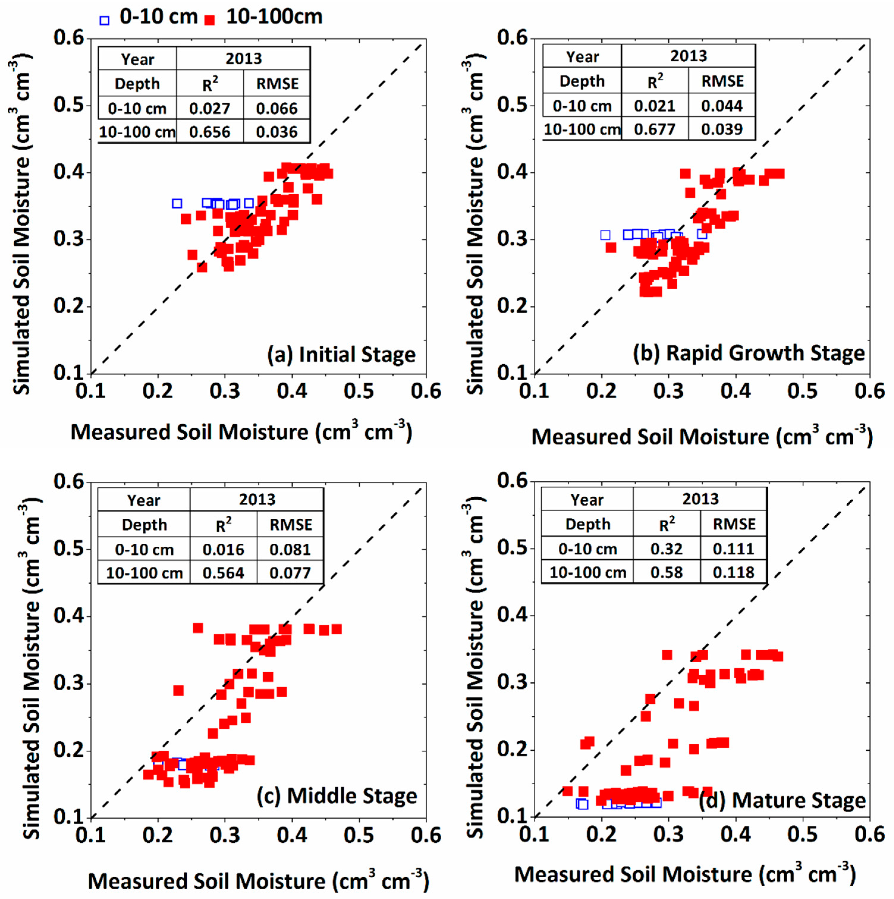
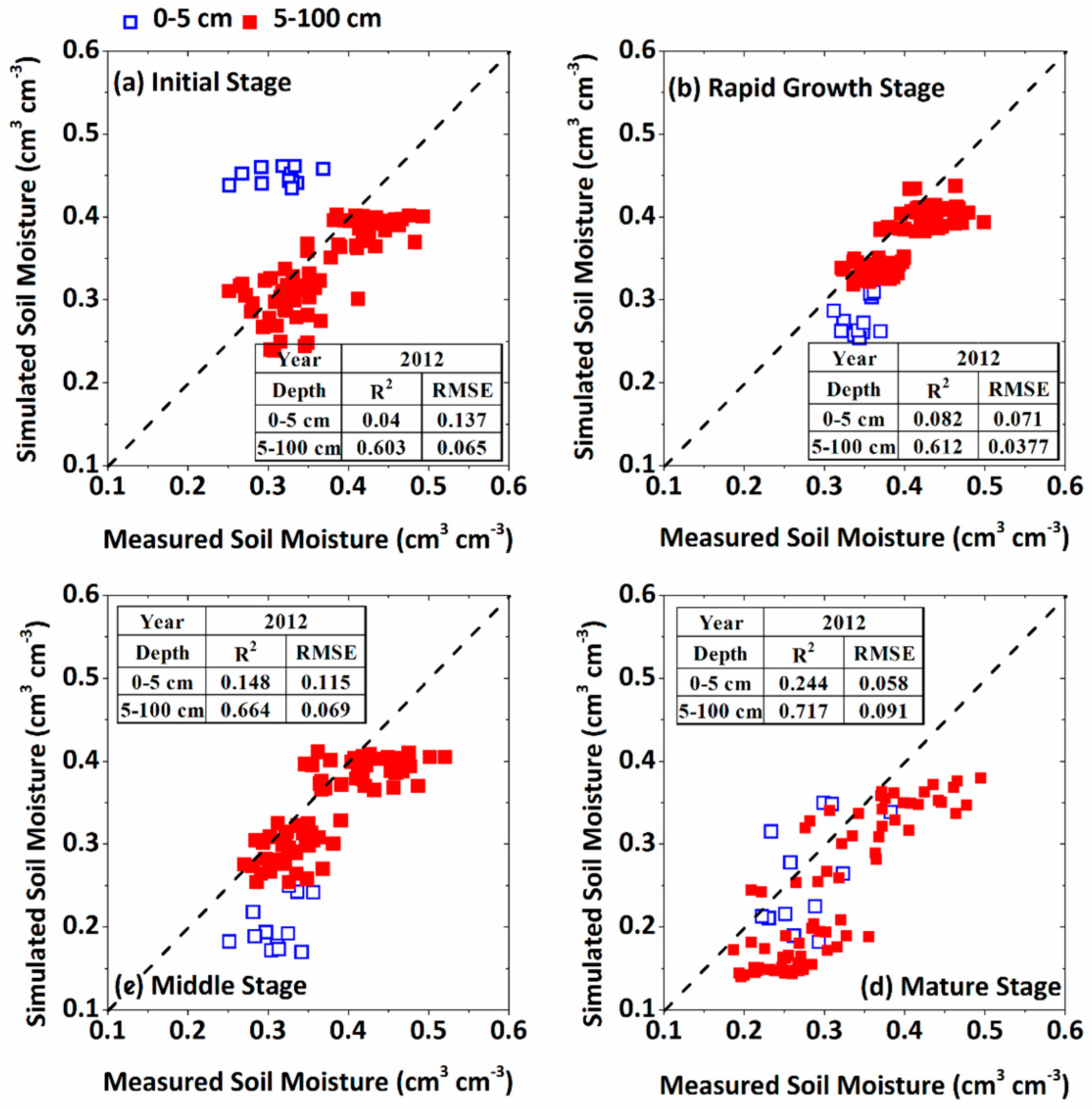
3.2. Calibration of the WFSP Model

Soil water flow and water uptake by sunflower were computed for a soil profile with 100-cm depth. The simulation period was from early June to late September, and conceded with the growth period of sunflowers. Model setup required specific daily precipitation and reference evapotranspiration as input data. The parameter calibration analysis was carried out using the main factors affecting the water regime (i.e., soil moisture, the cumulative values of actual transpiration and evaporation, capillary rise and other additional parameters) as the objective variables. After that, the above-mentioned sensitive parameters and some parameters introduced in Section 2.2 were calibrated using a trial-and-error method. An iterative calibration approach was adopted to account for the interactions between the measured soil moisture and simulated soil moisture. After proper calibration, the model was considered to be adequate for the evaluation of water movement in the soil-plant-atmosphere continuum (SPAC) system. The observed soil water contents in different soil layers relative to 2012 and 2013 were used to calibrate and validate the model, respectively. To assess the performance of the model, several goodness-of-fit indicators proposed in Section 2.3 were used as in the paper (e.g., R2 and RMSE). Based on the parameter sensitivity analysis, many parameters were only slightly adjusted depending on the goodness-of-fit indicators. The root water uptake parameters, including Feddes’ parameters and the basic soil parameters for sunflowers were calibrated and were shown in the former section. Some calibrated Kc values for sunflowers were slightly lower than those recommended in literature. This may due to the fact that the crop varieties planted in Hetao Irrigation District were more salt-tolerant than in the non-salinized area.
Soil moisture observed at different sunflower growth stages were well captured by the WFSP model except for the surface soil (0–5 cm) in the model calibration process (Figure 4, Year 2012). More exactly, R2 in initial, rapid growth, middle, and mature stages for 5–100 cm depth were 0.60, 0.61, 0.66, and 0.72 respectively while RMSE were only 0.07, 0.04, 0.07 and 0.09 cm3·cm−3 respectively.
Accumulative evapotranspiration (AETc) was also calculated, and the average AETc of the four growth stages were 77.1, 66.5, 156.2, and 44.3 mm respectively in 2012 (Figure 5a); and 60.0, 74.2, 123.6, and 19.7 mm respectively in 2013 (Figure 5b), indicating that the AETc of sunflowers was comparable in first two growth stages and achieved highest and lowest values in the middle and mature stages respectively.

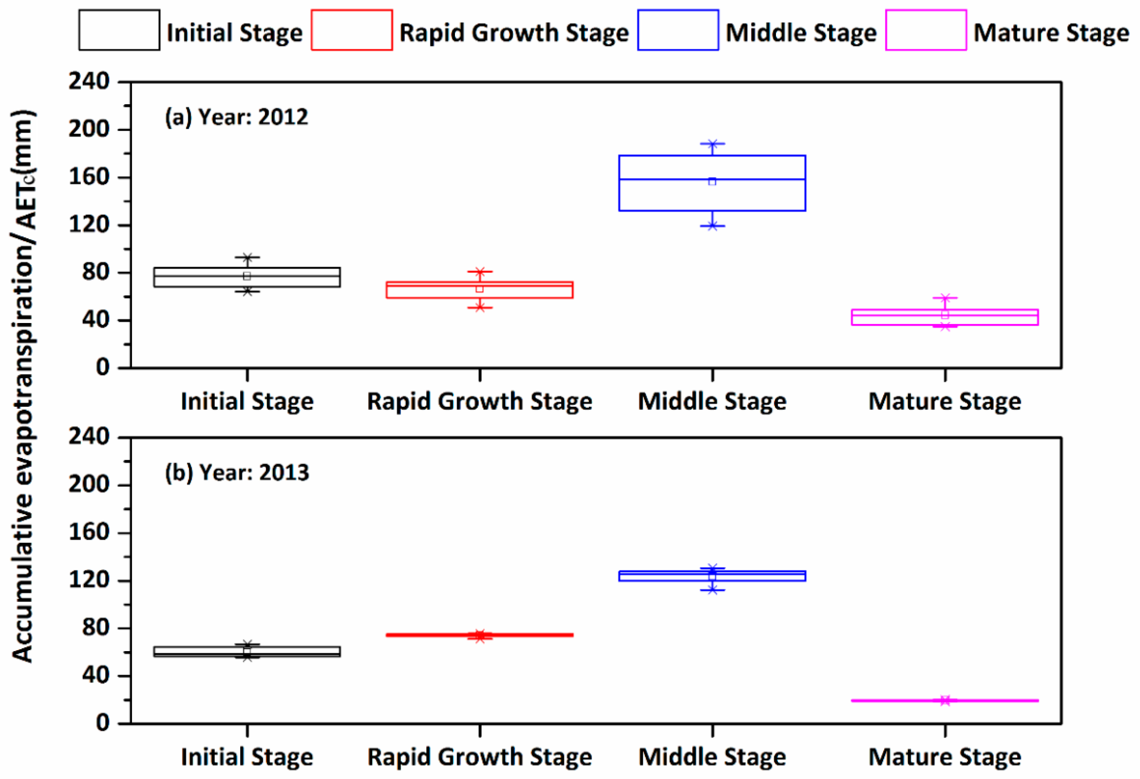
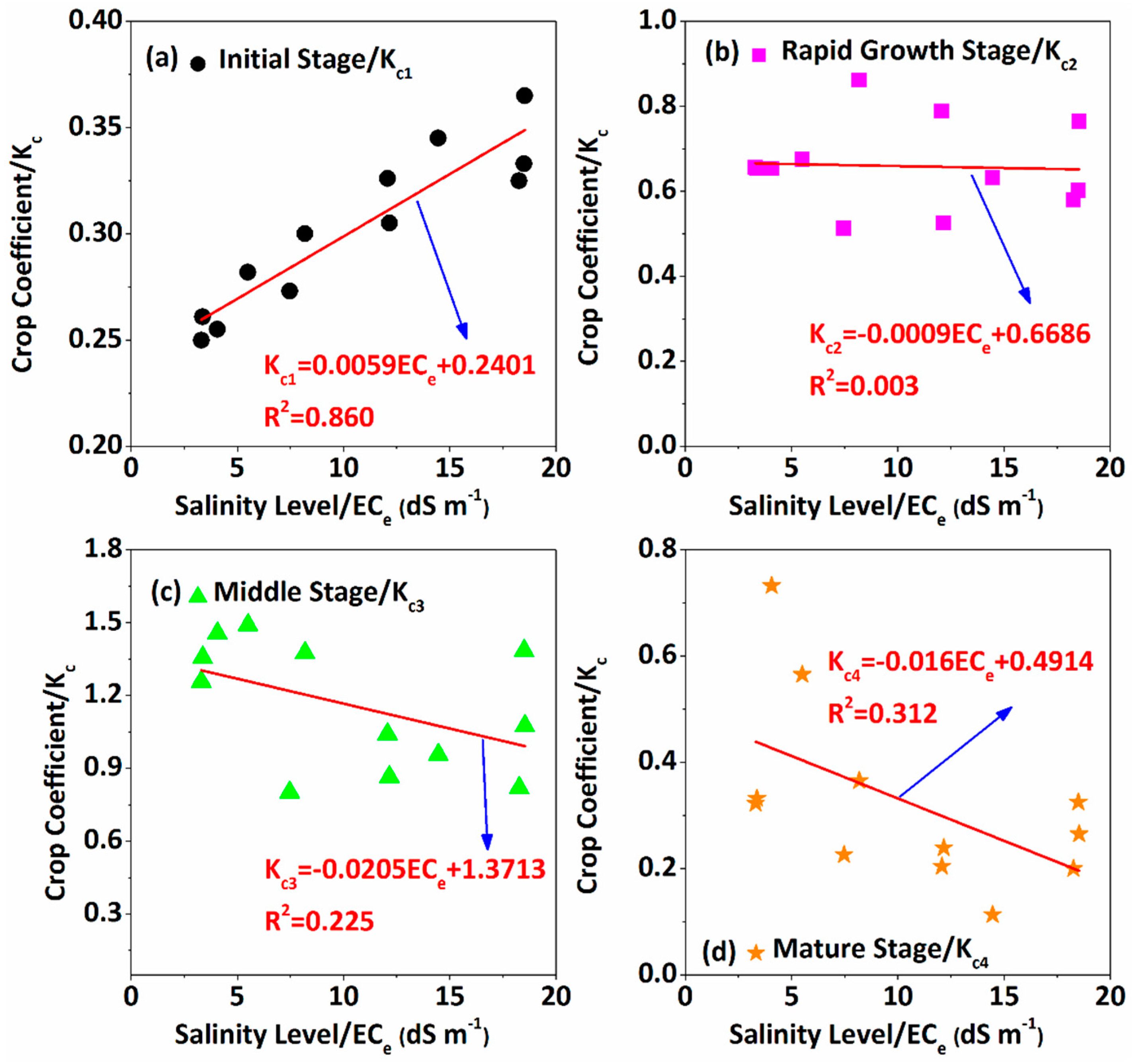
3.3. Establishment and Evaluation of the Locally-Based Sunflower Kc Values

Calibration of the WFSP model also indicates that Kc values for sunflowers in saline soils (ECe = 3.3–18.5 dS·m−1) ranged from 0.25–0.37, 0.51–0.86, 0.80–1.49, and 0.11–0.73 of initial (Kc1), rapid growth (Kc2), middle (Kc3), and mature stages (Kc4) respectively. Meanwhile, linear regression analysis indicated that all Kc values except Kc1 decreased with soil salinity levels (Figure 6). Furthermore, Kc1 had a very good linear correlation with the initial salinity level of 0–20 cm depth (Equation (20)).
K c 1 = 0.0059 E C e + 0.2401
Therefore, we assume that sunflower’s Kc1 value in saline soils could be easily obtained through Equation (20) while the locally-based Kc values for another three stages could be 0.51–0.86, 0.80–1.49, and 0.11–0.73 for use as reference values. To further simplify, we averaged the Kc2, Kc3, and Kc4 values obtained in our model (0.659, 1.156, and 0.324, respectively) and applied the WFSP model to evaluate their accuracy with the calculated Kc1 value (Equation (20)) using soil and weather conditions in 2013 (Figure 7). Similar to the model calibration process, higher accuracies for soil moisture simulations were also obtained for all four growth stages when the surface soils were ignored (0–10 cm in 2013). More exactly, R2 in the initial, rapid growth, middle, and mature stages for 10–100-cm depth were 0.66, 0.68, 0.56, and 0.58, respectively, while RMSEs were only 0.04, 0.04, 0.08 and 0.11 cm3·cm−3, respectively.

4. Discussion

4.1. Performance of the WFSP Model

Different from other models (e.g., HYDRUS) which use Richards equation to describe soil water flow [52,53], the WFSP model calculated water movement in the soil-plant system based on the water balance principle. The method is simpler than others and can overcome the iterative convergence issue when solving the Richards equation [54,55]. In our study, the WFSP model could simulate soil water dynamics accurately in both 2012 and 2013 except for the surface soils (Figure 4 and Figure 7, R2 > 0.56, RMSE < 0.1 cm3·cm−3). Meanwhile, the AETc values for the different growth stages of the sunflower calculated by the WFSP model were also similar to those in research by Ren et al. [56], Du et al. [25], and Xin et al. [57]. Therefore, the WFSP model could obtain reasonable simulations of soil water flow in the soil–plant system and could be used as a tool for analyzing the agro-hydrological processes and inverting the sunflower crop coefficient under salt stress. However, the poor accuracy for surface soil moisture simulation may be caused by the unusual weather conditions in 2012. In addition, the uncertainties of input data and field measurements such as groundwater table [58], the possible preferential flow [59] and even the observation errors might also bring adverse influences on the accuracy of the simulations for all four stages.

4.2. Sunflower’s Kc Values in Saline Soils

Crop coefficient (Kc) is a key parameter for estimating crop water use and to schedule irrigations [12]. In our study, Kc in the initial stage (Kc1) was determined by initial soil salinity of 0–20 cm depth due to a very high correlation (R2 = 0.86, Figure 6a). For the rapid growth, middle and mature stages, sunflower’s Kc were 0.659, 1.156, and 0.324, respectively. However, locally-based Kc values for sunflowers in saline soils proposed in our study (LKc) were different to previous research (Table 4). FAO-56 reported Kc values were 0.35, 1.0–1.15, and 0.35 for initial, middle and mature stages of sunflowers respectively [16]. LKc used four growth stages and were adjusted a little (<8%) in middle and mature stages, which increased R2 of soil moisture simulation (10–100 cm) for about 10% (Table 4) in moderately salinized soil (ECe = 9.44 dS·m−1). In India, Tyagi et al. [20] reported Kc values for sunflowers as 0.52, 1.1, 0.32 and 0.41, estimating Kc values 11.6%–74.2% higher than the values suggested by FAO-56, also different to our LKc values. Even for the same plants in close areas, Kc values may also be extremely different. In Hetao Irrigation District, Dai et al. [60] reported Kc values of 0.697, 0.751, 0.804, and 0.35, respectively for the four growth stages, with Kc values over 100% higher than ours in the initial stage, and about 30% lower in the middle stage. Du et al. [25] also obtained different Kc values for sunflowers compared to both Dai et al. [60] and our results (Table 4). The differences among Kc values might be caused from both soil and climate conditions and one of the most important factors was soil salinity [61,62]. Taking FAO-56 as an example, it deals with the calculation of crop evapotranspiration (ETc) under standard conditions. The values for Kc in FAO-56 are values for non-stressed crops cultivated under excellent agronomic and water management conditions and achieving maximum crop yield (standard conditions). Meanwhile, FAO-56 also ignores the difference among varieties. In addition, some specific agricultural practices such as plastic film covering the soil surface might also impact Kc determination. Therefore, FAO-56 strongly encouraged users to obtain appropriate local Kc values for a specific crop variety based on local soil and weather conditions. By considering salinity effects, LKc values obtained the highest accuracy for soil moisture simulation (R2 = 0.7) in moderately salinized soils when compared to previous research (Table 4).
In general, higher soil salinity results in lower Kc, which is also in accordance with our Kc2, Kc3, and Kc4 (Figure 6b–d). However, a very high positive correlation was found between Kc1 and salinity level (Figure 6a), which was unusual but also demonstrated that effects of salinity on Kc1 were more pronounced than in other stages. Similar results also obtained by Grattan and Grieve [63], who indicated that the initial stage of the crop was generally more salt sensitive than later growth stages and that crop failures during initial stages are common on saline lands. However, Bernstein and Hayward [64] reported that salt accumulations at seed depths are often much greater than at lower levels in the soil profile and when response to actual ambient salinity is considered, the initial stage is generally no more salt sensitive than later stages. Meanwhile, sunflowers were classified as moderately salt-tolerant plants by Katerji et al. [65] and previous studies also proved that a certain extent of salinity level might enhance sunflower growth [66]. Therefore, it is reasonable to believe that two or more of these processes with respect to the positive or negative effects of salinity on sunflowers may occur at the initial stage, but whether they ultimately affect Kc value or crop yield depends upon the salinity level, composition of salts, the crop species, and some other environmental factors which need further research.

5. Conclusions

Crop evapotranspiration calculation (ETc) plays a pivotal role in evaluating irrigation management strategies for improving agricultural water use, especially in saline regions. Appropriate irrigation schedules are of vital importance to adequately manage it. To determine ETc and make appropriate irrigation schedules, crop coefficients (Kc) have to be representatively determined. Based on soil moisture observations, a strong dynamics analysis tool (Vensim software) was used to establish and develop a physically-based model (WFSP model) for estimating the crop coefficients (Kc) of sunflowers in the Hetao Irrigation District. The two main findings were that firstly, only soil moisture data is needed for WFSP model, which makes this method more practical for developing an irrigation schedule. Meanwhile, the WFSP model could estimate reasonable simulations on the soil water flow in the soil–plant system and thus could be used as a tool for analyzing the agro-hydrological processes and deducing the sunflower crop coefficient under salt stress conditions. Secondly, our study indicates that the effects of salt stress on plant could be considered with Kc determination. Kc1 had a very good linear correlation with the initial salinity level of 0–20 cm depth (Equation (20)), and local-based Kc values for rapid growth, middle, and mature stages are recommended as 0.659, 1.156, and 0.324, respectively. These local crop coefficients could be very useful in irrigation schedules for local agricultural water managers.
However, there are still several shortcomings of our study. Firstly, soil salt dynamics were not considered in the study and further work should focus on the effects of salt dynamics with respect to Kc at the different crop stages. In addition, ECe was used to reflect the total salt content and the effects of salt composition on Kc and would need further study. Meanwhile, the LKc values for sunflowers, especially Equation (20) also need to be evaluated in other saline soils to test their stability and applicability.

Acknowledgments

This work was made possible by support from the State Natural Science Fund of China (Grant Nos. 51609175 and 51379151), Open Foundation of State Key Laboratory of Hydrology-Water Resources and Hydraulic Engineering (Grant No. 2015490211), the Fundamental Research Funds for the Central Universities (Grant Nos. 2042016kf0043 and 2042016kf1034), and the China Postdoctoral Science Foundation (Grant No. 2015M582274). Authors appreciate Yonggen Zhang’s help for proofreading the manuscript.

Author Contributions

The research present here was carried out in collaboration between all authors. Wenzhi Zeng, Minghai Hong and Jiesheng Huang conceived the idea and designed the study; Minghai Hong carried out the data analysis, set up the model, and prepared the first draft of the manuscript; Wenzhi Zeng and Yuanhao Fang were also of vital importance in revising the manuscript; and Tao Ma, Guoqing Lei, Yuanyuan Zha, Jingwei Wu and Jiesheng Huang provided important advice on the concept writing of the manuscript and English grammar.

Conflicts of Interest

The authors declare no conflict of interest.

References

  1. Demir, A.O.; Goksoy, A.T.; Buyukcangaz, H.; Turan, Z.M.; Koksal, E.S. Deficit irrigation of sunflower (Helianthus annuus L.) in a sub-humid climate. Irrig. Sci. 2006, 24, 279–289. [Google Scholar] [CrossRef]
  2. Shi, H.; Akae, A.; Kong, D.; Zhang, L.; Chen, Y.; Wei, Z.; Li, Y.; Zhang, Y. In study on sunflower response to soil water and salt stress in the Hetao area, China. In Water-Saving Agriculture and Sustainable use of Water and Land Resources; Shaanxi Science and Technology Press: Xi’an, China, 2003; pp. 111–116. [Google Scholar]
  3. Feng, Z.Z.; Wang, X.K.; Feng, Z.W. Soil n and salinity leaching after the autumn irrigation and its impact on groundwater in Hetao irrigation district, China. Agric. Water Manag. 2005, 71, 131–143. [Google Scholar] [CrossRef]
  4. Li, L.; Shi, H.; Wang, C.; Liu, H. Simulation of water and salt transport of uncultivated land in Hetao irrigation district in Inner Mongolia. Trans. Chin. Soc. Agric. Eng. 2010, 26, 31–35. [Google Scholar]
  5. Ertek, A.; Kara, B. Yield and quality of sweet corn under deficit irrigation. Agric. Water Manag. 2013, 129, 138–144. [Google Scholar] [CrossRef]
  6. Cakir, R. Effect of water stress at different development stages on vegetative and reproductive growth of corn. Field Crop Res. 2004, 89, 1–16. [Google Scholar] [CrossRef]
  7. Dagdelen, N.; Yilmaz, E.; Sezgin, F.; Gurbuz, T. Water-yield relation and water use efficiency of cotton (Gossypium hirsutum L.) and second crop corn (Zea mays L.) in western Turkey. Agric. Water Manag. 2006, 82, 63–85. [Google Scholar] [CrossRef]
  8. Irmak, S.; Djaman, K.; Rudnick, D.R. Effect of full and limited irrigation amount and frequency on subsurface drip-irrigated maize evapotranspiration, yield, water use efficiency and yield response factors. Irrig. Sci. 2016, 34, 271–286. [Google Scholar] [CrossRef]
  9. Kiziloglu, F.M.; Sahin, U.; Kuslu, Y.; Tunc, T. Determining water-yield relationship, water use efficiency, crop and pan coefficients for silage maize in a semiarid region. Irrig. Sci. 2009, 27, 129–137. [Google Scholar] [CrossRef]
  10. Payero, J.O.; Melvin, S.R.; Irmak, S.; Tarkalson, D. Yield response of corn to deficit irrigation in a semiarid climate. Agric. Water Manag. 2006, 84, 101–112. [Google Scholar] [CrossRef]
  11. Zeng, W.Z.; Xu, C.; Wu, J.W.; Huang, J.S. Soil salt leaching under different irrigation regimes: HYDRUS-1D modelling and analysis. J. Arid Land 2014, 6, 44–58. [Google Scholar] [CrossRef]
  12. Alcaras, L.M.A.; Rousseaux, M.C.; Searles, P.S. Responses of several soil and plant indicators to post-harvest regulated deficit irrigation in olive trees and their potential for irrigation scheduling. Agric. Water Manag. 2016, 171, 10–20. [Google Scholar] [CrossRef]
  13. Pereira, L.S.; Allen, R.G.; Smith, M.; Raes, D. Crop evapotranspiration estimation with FAO56: Past and future. Agric. Water Manag. 2015, 147, 4–20. [Google Scholar] [CrossRef]
  14. Vellidis, G.; Tucker, M.; Perry, C.; Wen, C.; Bednarz, C. A real-time wireless smart sensor array for scheduling irrigation. Comput. Electron. Agric. 2008, 61, 44–50. [Google Scholar] [CrossRef]
  15. Jones, H.G. Irrigation scheduling: Advantages and pitfalls of plant-based methods. J. Exp. Bot. 2004, 55, 2427–2436. [Google Scholar] [CrossRef] [PubMed]
  16. Allen, R.G.; Pereira, L.S.; Raes, D.; Smith, M. Crop Evapotranspiration-guidelines for Computing Crop Water Requirements-FAO Irrigation and Drainage Paper 56; FAO: Rome, Italy, 1998; p. D05109. [Google Scholar]
  17. Jensen, M.E. Water consumption by agricultural plants (Chapter 1). In Plant Water Consumption and Response. Water Deficits and Plant Growth; Academic Press: New York, NY, USA, 1968; Volume II, pp. 1–22. [Google Scholar]
  18. Howell, T.A.; Evett, S.R.; Tolk, J.A.; Copeland, K.S.; Marek, T.H. Evapotranspiration, water productivity and crop coefficients for irrigated sunflower in the US southern high plains. Agric. Water Manag. 2015, 162, 33–46. [Google Scholar] [CrossRef]
  19. Reddy, K.C.; Arunajyothy, S.; Mallikarjuna, P. Crop coefficients of some selected crops of Andhra Pradesh. J. Inst. Eng. (India): Ser. A 2015, 96, 123–130. [Google Scholar] [CrossRef]
  20. Tyagi, N.K.; Sharma, D.K.; Luthra, S.K. Determination of evapotranspiration and crop coefficients of rice and sunflower with lysimeter. Agric. Water Manag. 2000, 45, 41–54. [Google Scholar] [CrossRef]
  21. Zeng, W.Z.; Xu, C.; Huang, J.S.; Wu, J.W.; Ma, T. Emergence rate, yield, and nitrogen-use efficiency of sunflowers (Helianthus annuus) vary with soil salinity and amount of nitrogen applied. Commun. Soil Sci. Plant Anal. 2015, 46, 1006–1023. [Google Scholar] [CrossRef]
  22. Zeng, W.Z.; Xu, C.; Wu, J.W.; Huang, J.S.; Zhao, Q.; Wu, M.S. Impacts of salinity and nitrogen on the photosynthetic rate and growth of sunflowers (Helianthus annuus L.). Pedosphere 2014, 24, 635–644. [Google Scholar] [CrossRef]
  23. Zeng, W.Z.; Wu, J.W.; Hoffmann, M.P.; Xu, C.; Ma, T.; Huang, J.S. Testing the apsim sunflower model on saline soils of Inner Mongolia, China. Field Crop Res. 2016, 192, 42–54. [Google Scholar] [CrossRef]
  24. Bhantana, P.; Lazarovitch, N. Evapotranspiration, crop coefficient and growth of two young pomegranate (Punica granatum L.) varieties under salt stress. Agric. Water Manag. 2010, 97, 715–722. [Google Scholar] [CrossRef]
  25. Du, B.; Qu, Z.; Yu, J.; Sun, G.; Shi, J. Experimental study on crop coefficient under mulched drip irrigation in Hetao irrigation district of Inner Mongolia. J. Irrig. Drain. 2014, 33, 16–20. [Google Scholar]
  26. Miller, W.P.; Miller, D.M. A micro-pipette method for soil mechanical analysis. Commun. Soil Sci. Plant Anal. 1987, 18, 1–15. [Google Scholar] [CrossRef]
  27. Bao, S.D. Soil Agro-Chemistrical Analysis, 3rd ed.; China Agriculture Press: Beijing, China, 2011; p. 496. [Google Scholar]
  28. Institute of Soil Science. Analysis of Soil Physico-Chemical Properties; Shanghai Scientific & Technical Publishers: Shanghai, China, 1978. [Google Scholar]
  29. Forrester, J.W. Industrial dynamics: A major breakthrough for decision makers. Harv. Bus. Rev. 1958, 37–66. [Google Scholar]
  30. Forrester, J.W. Industrial Dynamics; MIT Press: Cambridge, UK, 1961. [Google Scholar]
  31. Khan, S.; Luo, Y.F.; Ahmad, A. Analysing complex behaviour of hydrological systems through a system dynamics approach. Environ. Modell. Softw. 2009, 24, 1363–1372. [Google Scholar] [CrossRef]
  32. Miller, G.R.; Cable, J.M.; McDonald, A.K.; Bond, B.; Franz, T.E.; Wang, L.X.; Gou, S.; Tyler, A.P.; Zou, C.B.; Scott, R.L. Understanding ecohydrological connectivity in savannas: A system dynamics modelling approach. Ecohydrology 2012, 5, 200–220. [Google Scholar] [CrossRef] [Green Version]
  33. Yang, C.-C.; Chang, L.-C.; Ho, C.-C. Application of system dynamics with impact analysis to solve the problem of water shortages in Taiwan. Water Resour. Manag. 2008, 22, 1561–1577. [Google Scholar] [CrossRef]
  34. Eberlein, R.L.; Peterson, D.W. Understanding models with Vensim™. Eur. J. Oper. Res. 1992, 59, 216–219. [Google Scholar] [CrossRef]
  35. Systems, V. Vensim Reference Mannual; Ventana Systems: Harvard, MA, USA, 2007. [Google Scholar]
  36. Systems, V. Vensim Version 5 User’s Guide; Ventana Systems: Harvard, MA, USA, 2007. [Google Scholar]
  37. Igboekwe, M.U.; Adindu, R.U. Use of Kostiakov’s Infiltration Model on Michael Okpara University of Agriculture, Umudike Soils, Southeastern, Nigeria. J. Water Resour. Prot. 2014, 6, 888–894. [Google Scholar] [CrossRef]
  38. Vangenuchten, M.T. A closed-form equation for predicting the hydraulic conductivity of unsaturated soils. Soil Sci. Soc. Am. J. 1980, 44, 892–898. [Google Scholar] [CrossRef]
  39. Vangenuchten, M.T.; Nielsen, D.R. On describing and predicting the hydraulic-properties of unsaturated soils. Ann. Geophys. 1985, 3, 615–627. [Google Scholar]
  40. Schaap, M.G.; Leij, F.J.; van Genuchten, M.T. ROSETTA: A computer program for estimating soil hydraulic parameters with hierarchical pedotransfer functions. J. Hydrol. 2001, 251, 163–176. [Google Scholar] [CrossRef]
  41. Liang, J.; Li, R.; Shi, H.; Li, Z.; Lu, X.; Bu, H. Effect of mulching on transfer and distribution of salinizated soil nutrient in Hetao irrigation district. Trans. Chin. Soc. Agric. Mach. 2016, 2, 113–121. [Google Scholar]
  42. Li, F. Experimental study of groudwater availability in relation to crops. Groundwater 1992, 197–202. [Google Scholar]
  43. Feng, G.; Liu, C. Analysis of root system growth in relation to soil water extraction pattern by winter wheat under water-limiting conditions. J. Nat. Resour. 1998, 3, 234–241. [Google Scholar]
  44. Chen, H.; Gao, Z.; Wang, S.; Hu, Y. Modeling on impacts of climate change and human activities variability on the shallow groundwater level using modflow. J. Hydraul. Eng. 2012, 43, 344–353. [Google Scholar]
  45. Gale, M.R.; Grigal, D.F. Vertical root distributions of northern tree species in relation to successional status. Can. J. For. Res. 1987, 17, 829–834. [Google Scholar] [CrossRef]
  46. Jackson, R.B.; Canadell, J.; Ehleringer, J.R.; Mooney, H.A.; Sala, O.E.; Schulze, E.D. A global analysis of root distributions for terrestrial biomes. Oecologia 1996, 108, 389–411. [Google Scholar] [CrossRef]
  47. Feddes, R.A.; Kowalik, P.J.; Zaradny, H. Simulation of field water use and crop yield. Soil Sci. 1980, 129, 193. [Google Scholar]
  48. Feddes, R.A.; Kowalik, P.; Kolinska-Malinka, K.; Zaradny, H. Simulation of field water uptake by plants using a soil water dependent root extraction function. J. Hydrol. 1976, 31, 13–26. [Google Scholar] [CrossRef]
  49. Zhang, M.; Shi, X. Soil and Crop Science; China Water & Power Press: Beijing, China, 2012. [Google Scholar]
  50. Putnam, H. Trial and error predicates and the solution to a problem of Mostowski. J. Symb. Logic 1965, 30, 49–57. [Google Scholar] [CrossRef]
  51. Yuting, Y.; Songhao, S. Comparison of dual-source evapotranspiration models in estimating potential evaporation and transpiration. Trans. Chin. Soc. Agric. Eng. 2012, 28, 85–91. [Google Scholar]
  52. Šimůnek, J.; Van Genuchten, M.T.; Sejna, M. The Hydrus-1d Software Package for Simulating the Movement of Water, Heat, and Multiple Solutes in Variably Saturated Media, Version 3.0, Hydrus Software Series 1; Department of Environmental Sciences, University of California Riverside: Riverside, CA, USA, 2005. [Google Scholar]
  53. Zhang, Z.Y.; Wang, W.K.; Yeh, T.C.J.; Chen, L.; Wang, Z.F.; Duan, L.; An, K.D.; Gong, C.C. Finite analytic method based on mixed-form richards’ equation for simulating water flow in vadose zone. J. Hydrol. 2016, 537, 146–156. [Google Scholar] [CrossRef]
  54. Zha, Y.Y.; Shi, L.S.; Ye, M.; Yang, J.Z. A generalized ross method for two- and three-dimensional variably saturated flow. Adv. Water Resour. 2013, 54, 67–77. [Google Scholar] [CrossRef]
  55. Zha, Y.Y.; Yang, J.Z.; Shi, L.S.; Song, X.H. Simulating one-dimensional unsaturated flow in heterogeneous soils with water content-based richards equation. Vadose Zone J. 2013, 12, 1–13. [Google Scholar] [CrossRef]
  56. Ren, D.; Xu, X.; Hao, Y.; Huang, G. Modeling and assessing field irrigation water use in a canal system of Hetao, upper Yellow River basin: Application to maize, sunflower and watermelon. J. Hydrol. 2016, 532, 122–139. [Google Scholar] [CrossRef]
  57. He, X.; Yang, P.L.; Ren, S.M.; Li, Y.K.; Jiang, G.Y.; Li, L.H. Quantitative response of oil sunflower yield to evapotranspiration and soil salinity with saline water irrigation. Int. J. Agric. Biol. Eng. 2016, 9, 63–73. [Google Scholar]
  58. Sun, M.; Zhang, X.; Huo, Z.; Feng, S.; Huang, G.; Mao, X. Uncertainty and sensitivity assessments of an agricultural–hydrological model (RZWQM2) using the GLUE method. J. Hydrol. 2016, 534, 19–30. [Google Scholar] [CrossRef]
  59. Wiekenkamp, I.; Huisman, J.A.; Bogena, H.R.; Lin, H.S.; Vereecken, H. Spatial and temporal occurrence of preferential flow in a forested headwater catchment. J. Hydrol. 2016, 534, 139–149. [Google Scholar] [CrossRef]
  60. Dai, J.; Shi, H.; Tian, D.; Xia, Y.; Li, M. Determined of crop coefficients of main grain and oil crops in Inner Mongolia Hetao irrigated area. J. Irrig. Drain. 2011, 23–27. [Google Scholar]
  61. Homaee, M.; Dirksen, C.; Feddes, R.A. Simulation of root water uptake: I. Non-uniform transient salinity using different macroscopic reduction functions. Agric. Water Manag. 2002, 57, 89–109. [Google Scholar] [CrossRef]
  62. Skaggs, T.H.; van Genuchten, M.T.; Shouse, P.J.; Poss, J.A. Macroscopic approaches to root water uptake as a function of water and salinity stress. Agric. Water Manag. 2006, 86, 140–149. [Google Scholar] [CrossRef]
  63. Grattan, S.R.; Grieve, C.M. Salinity mineral nutrient relations in horticultural crops. Sci. Hortic-Amst. 1999, 78, 127–157. [Google Scholar] [CrossRef]
  64. Bernstein, L.; Hayward, H. Physiology of salt tolerance. Annu. Rev. Plant Physiol. 1958, 9, 25–46. [Google Scholar] [CrossRef]
  65. Katerji, N.; van Hoorn, J.W.; Hamdy, A.; Mastrorilli, M. Salt tolerance classification of crops according to soil salinity and to water stress day index. Agric. Water Manag. 2000, 43, 99–109. [Google Scholar] [CrossRef]
  66. Zeng, W.Z. Research and Simulation for the Coupling Effects of Water, Nitrogen, and Salt on Sunflower; Wuhan University: Wuhan, China, 2015. [Google Scholar]
Figure 1. The location site (a) of the experimental study area. The green dot is the location of subplots at the Yichang Experimental Station. The arrangement of the trial blocks are depicted in (b) with the schematic diagram of the block profile (c) and plant arrangement (d) within each block (units in cm) also being shown.
Water 09 00215 g001
Figure 2. Basic model framework. P is precipitation (mm); C is the capillary water movement into the soil layer (mm); I is the seepage movement out of the soil layer (mm); E is soil evaporation (mm); and U is root water uptake from the soil layer (mm). RO is the surface runoff (mm). RW is the groundwater recharge (mm); FW is the water flow out of the whole root zone (mm). Subscript i indicates the layer number.
Water 09 00215 g002
Figure 3. Precipitation and potential evapotranspiration (ET0) of sunflower growing seasons in 2012 (a) and 2013 (b). Red curves are the parabolic fitting of the ET0.
Water 09 00215 g003
Figure 4. Soil moisture simulation of sunflowers at four different growth stages of model calibration using the observations in 2012 ((a): initial stage; (b): rapid growth stage; (c): middle stage; (d): mature stage; blue points indicate observations in 0–5 cm and red points indicate observations in 5–100 cm). RMSE: root-mean-square error.
Water 09 00215 g004
Figure 5. Box plot of accumulative evapotranspiration (AETc) of the four growth stages of sunflowers in 2012 (a) and 2013 (b) respectively. The line in the box is the median, the edges of the box are the lower hinge (25%, Q1) and the upper hinge (75%, Q3), the up and low boundary lines out of the box indicate the maximum and minimum values and the cross symbols near the up and low boundaries are the 99% and 1% hinges respectively.
Water 09 00215 g005
Figure 6. The relationship between the crop coefficient/Kc of sunflowers simulated by WFSP model and initial salinity level/ECe (dS·m−1) of 0–20 cm depth.
Water 09 00215 g006
Figure 7. Soil moisture simulation of sunflowers in four different growth stages for model evaluation using the observations in 2013 ((a): initial stage; (b): rapid growth stage; (c): middle stage; (d): mature stage; blue points indicate observations in 0–10 cm and red points indicate observations in 10–100 cm).
Water 09 00215 g007
Table 1. Soil physical properties of experimental area.
Depth (cm)Soil Particle Size Distribution/Mean ± S.D.* (%)Bulk Density (g/cm3)
Sand (0.05–2.0 mm)Silt (0.002–0.05 mm)Clay (< 0.002 mm)
0–1012.58 ± 4.3054.94 ± 12.1332.48 ± 13.861.35
10–2011.79 ± 3.9752.81 ± 13.5335.40 ± 14.671.35
20–3012.02 ± 4.2452.32 ± 12.4335.66 ± 14.051.35
30–4012.27 ± 6.8653.77 ± 12.1033.96 ± 15.491.44
40–608.91 ± 12.9669.77 ± 11.4121.32 ± 12.291.48
60–8012.48 ± 13.9170.57 ± 11.8016.95 ± 10.611.51
80–10016.69 ± 16.6969.59 ± 13.2813.72 ± 6.171.51
Note: * S.D. indicates standard deviation.
Table 2. Parameters of Equations (5) and (6) for the model. θr: residual soil moisture; θs: saturated soil moisture.
DepthθrθsαnKs
cm3·cm−3cm3·cm−31/cm-mm/d
0–10 cm0.0883 0.4691 0.0082 1.5057 121.9
10–20 cm0.0919 0.4774 0.0093 1.4737 125.4
20–30 cm0.0921 0.4776 0.0094 1.4702 125.9
30–40 cm0.0901 0.4733 0.0087 1.4893 123.5
40–60 cm0.0763 0.4540 0.0058 1.6156 131.2
60–80 cm0.0687 0.4477 0.0051 1.6582 176.0
80–100 cm0.0616 0.4431 0.0046 1.6903 235.6
Notes: θr and θs are the residual and saturated soil moistures (cm3·cm−3) respectively; Ks is the saturated hydraulic conductivity (mm·d−1); α and n are dimensionless empirical parameters.
Table 3. List of Feddes model parameters.
ParameterUnitsRangeValueDescriptionReference
θwiltcm3·cm−30.06–0.100.10Wilting point[49]
θfccm3·cm−30.32–0.420.39Field capacity[49]
θstresscm3·cm−3(0.45–0.9)·θfc0.6·θfcStress point[32]
Table 4. Comparison of crop coefficients/Kc between different researchers and our model in moderately salinized soil (ECe = 9.44 dS·m−1).
ItemInitial StageRapid Growth StageMiddle StageMature StageR2LocationReference
10.521.11.320.410.55Karnal, India (29°43′ N, 76°58′ E)[20]
20.6970.7510.8040.350.55Dengkou County, Hetao (40°24′ N, 107°02′ E)[60]
30.1940.7791.260.3150.67Linhe County, Hetao (40°43′ N, 76°58′ E)[25]
40.141.080.240.66Yangchang, Hetao (40°48′ N, 107°05′ E)[56]
50.351–1.150.350.64California, US[16]
6Equation (20)0.6591.1560.3240.7Wuyuan County, Hetao (41°04′ N, 108°00′ E)WFSP model

