Fifteen Years (1993–2007) of Surface Freshwater Storage Variability in the Ganges-Brahmaputra River Basin Using Multi-Satellite Observations

 , , ,
, , , 
Abstract
:1. Introduction
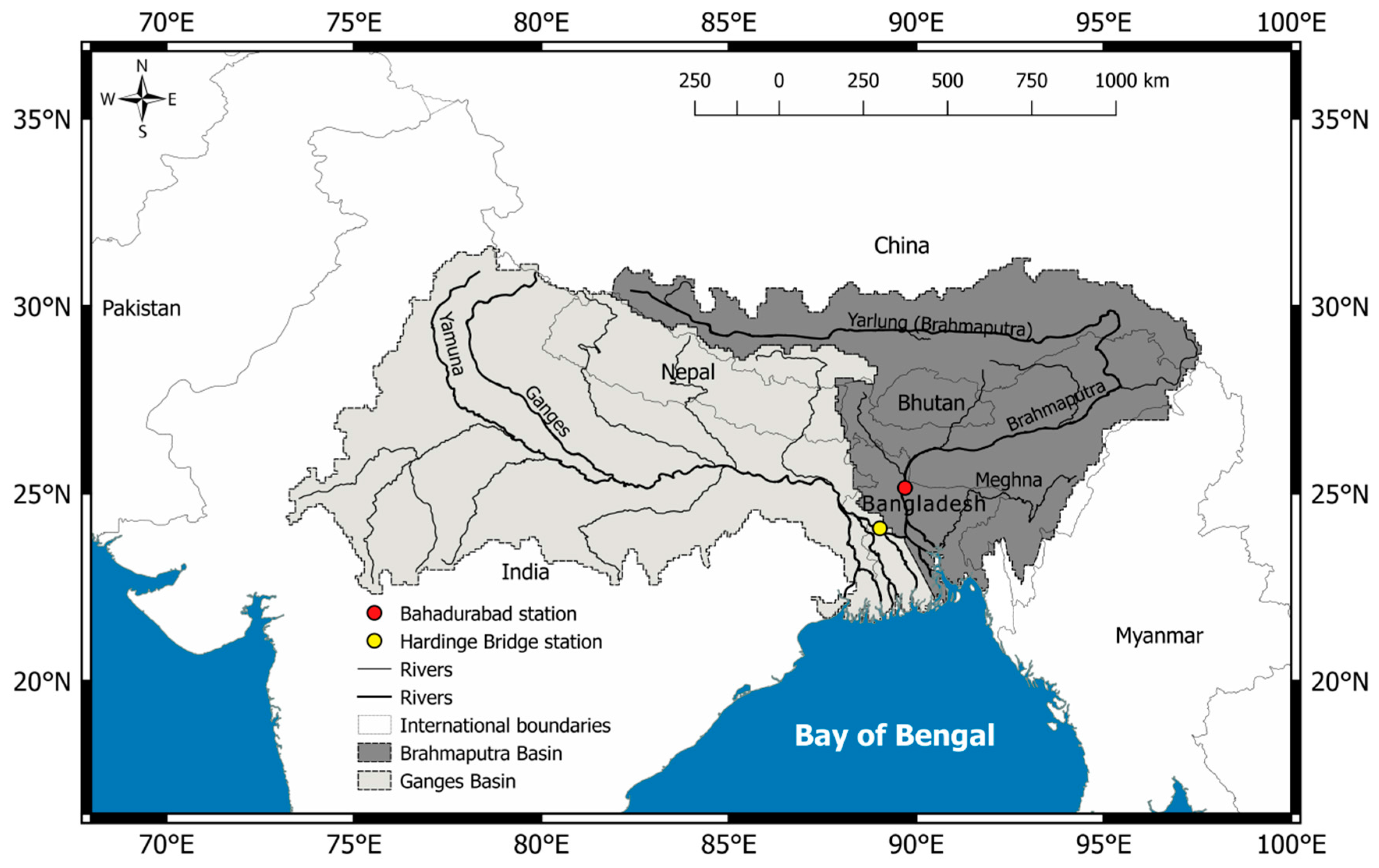
2. Study Area
3. Datasets
3.1. Global Inundation Extent from Multi-Satellites (GIEMS)
3.2. ASTER-GDEM to Derive Hypsographic Curves
3.3. SRTM-GDEM to Derive Hypsographic Curves as Used in CaMa-Flood and HyMAP Models
3.4. Complementary Datasets Used for Validation
3.4.1. Multi-Satellite Surface Water Storage from GIEMS and ENVISAT Radar Altimeter
3.4.2. GRACE Level-2 Monthly Solutions
3.4.3. GPCP Monthly Rainfall Product
3.4.4. River Discharges
4. Methods
4.1. GIEMS Surface Water Extent Thresholding
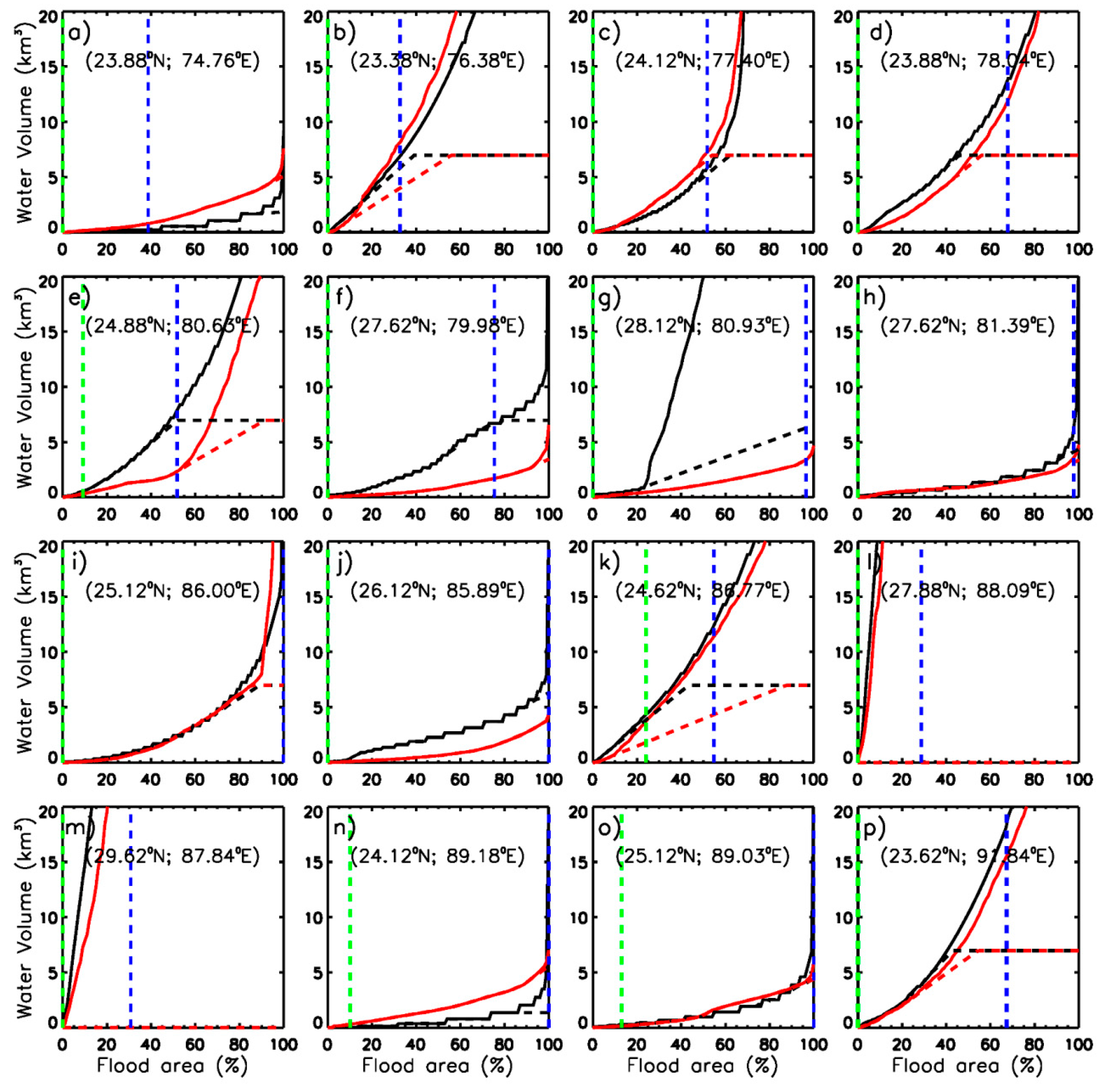
4.2. The Hypsographic Curve Approach
- The first step is to construct the hypsographic curve for each pixel of the surface water extent dataset (GIEMS). The corresponding GDEM elevation points for each pixel of GIEMS product (equal-grid of 773 km2) are selected. The elevation distribution function is then created and converted (by integration) to a curve of cumulative frequencies. The latter function presents the so-called hypsographic curve that consists of an area-elevation relationship, constructed for each pixel of the GIEMS data set.
- In the second step, a translation is applied to set to zero the lowest elevation of the hypsographic curve by subtracting the lowest value from all other elevations. The hypsographic curve is then converted into an area-surface water volume relationship by estimating the surface water volume associated with an increase of the pixel fractional open water coverage by filling the hypsographic curve from its base level to an upward level, following [13]:where is the surface water volume (in km3) for a percentage of flood/inundation (an increment i of 1% in percentage of inundation is chosen), is the area of a GIEMS pixel (773 km2), and h the elevation (in km) for a percentage of flood/inundation given by the hypsographic curve.
- In the last step, the surface water storage of each pixel is estimated for each month by combining the hypsographic curve with the monthly variations of surface water extent from GIEMS using Equation (2). The estimated surface water storages are not absolute. They correspond to the water volume present over a reference surface that is the topography or the elevation of the surface corresponding to the minimum water levels during the observation period. Thus, the estimated water storage represents the increment above the minimum storage.
4.3. Time Series of Basin Scale Total Water Storage (TWS)
5. Results and Discussion
6. Conclusions
Acknowledgments
Author Contributions
Conflicts of Interest
References
- Chahine, M.T. The hydrological cycle and its influence on climate. Nature 1992, 359, 373–380. [Google Scholar] [CrossRef]
- Papa, F.; Prigent, C.; Aires, F.; Jimenez, C.; Rossow, W.B.; Matthews, E. Interannual variability of surface water extent at the global scale, 1993–2004. J. Geophys. Res. 2010, 115, 1–17. [Google Scholar] [CrossRef]
- Alsdorf, D.E.; Rodriguez, E.; Lettenmaier, D.P. Measuring surface water from space. Rev. Geophys. 2007, 45, 1–24. [Google Scholar] [CrossRef]
- Frappart, F.; Papa, F.; Santos da Silva, J.; Ramillien, G.; Prigent, C.; Seyler, F.; Calmant, S. Surface freshwater storage and dynamics in the Amazon basin during the 2005 exceptional drought. Environ. Res. Lett. 2012, 7, 044010. [Google Scholar] [CrossRef]
- Prigent, C.; Papa, F.; Aires, F.; Jimenez, C.; Rossow, W.B.; Matthews, E. Changes in land surface water dynamics since the 1990s and relation to population pressure. Geophys. Res. Lett. 2012, 39, 2–6. [Google Scholar] [CrossRef]
- Prigent, C.; Papa, F.; Aires, F.; Rossow, W.B.; Matthews, E. Global inundation dynamics inferred from multiple satellite observations, 1993–2000. J. Geophys. Res. 2007, 112. [Google Scholar] [CrossRef]
- Frappart, F.; Do Minh, K.; L’Hermitte, J.; Cazenave, A.; Ramillien, G.; Le Toan, T.; Mognard-Campbell, N. Water volume change in the lower Mekong from satellite altimetry and imagery data. Geophys. J. Int. 2006, 167, 570–584. [Google Scholar] [CrossRef]
- Birkett, C.M. The contribution of TOPEX/POSEIDON to the global monitoring of climatically sensitive lakes. J. Geophys. Res. 1995, 100, 25179–25204. [Google Scholar] [CrossRef]
- Frappart, F.; Papa, F.; Famiglietti, J.S.; Prigent, C.; Rossow, W.B.; Seyler, F. Interannual variations of river water storage from a multiple satellite approach: A case study for the Rio Negro River basin. J. Geophys. Res. Atmos. 2008, 113, 1–12. [Google Scholar] [CrossRef]
- Frappart, F.; Calmant, S.; Cauhopé, M.; Seyler, F.; Cazenave, A. Preliminary results of ENVISAT RA-2-derived water levels validation over the Amazon basin. Remote Sens. Environ. 2006, 100, 252–264. [Google Scholar] [CrossRef]
- Frappart, F.; Papa, F.; Guntner, A.; Werth, S.; Ramillien, G.; Prigent, C.; Rossow, W.B.; Bonnet, M.P. Interannual variations of the terrestrial water storage in the lower Ob’ basin from a multisatellite approach. Hydrol. Earth Syst. Sci. 2010, 14, 2443–2453. [Google Scholar] [CrossRef]
- Frappart, F.; Papa, F.; Malbéteau, Y.; Leon, J.G.; Ramillien, G.; Prigent, C.; Seoane, L.; Seyler, F.; Calmant, S. Surface freshwater storage variations in the Orinoco floodplains using multi-satellite observations. Remote Sens. 2015, 7, 89–110. [Google Scholar] [CrossRef]
- Papa, F.; Frappart, F.; Malbéteau, Y.; Shamsudduha, M.; Vuruputur, V.; Sekhar, M.; Ramillien, G.; Prigent, C.; Aires, F.; Pandey, R.K.; et al. Satellite-derived surface and sub-surface water storage in the Ganges-Brahmaputra River Basin. J. Hydrol. Reg. Stud. 2015, 4, 15–35. [Google Scholar] [CrossRef]
- Papa, F.; Frappart, F.; Guntner, A.; Prigent, C.; Aires, F.; Getirana, A.C.V.; Maurer, R. Surface freshwater storage and variability in the Amazon basin from multi-satellite observations, 1993–2007. J. Geophys. Res. Atmos. 2013, 118, 11951–11965. [Google Scholar] [CrossRef]
- Chowdhury, R.; Ward, N. Hydro-meteorological variability in the greater Ganges-Brahmaputra-Meghna basins. Int. J. Climatol. 2004, 24, 1495–1508. [Google Scholar] [CrossRef]
- Gain, A.K.; Wada, Y. Assessment of future water scarcity at different spatial and temporal scales of the Brahmaputra River Basin. Water Resour. Manag. 2014, 28, 999–1012. [Google Scholar] [CrossRef]
- Winkel, L.; Berg, M.; Amini, M.; Hug, S.J.; Johnson, C.A. Predicting groundwater arsenic contamination in Southeast Asia from surface parameters. Nat. Geosci. 2008, 1, 536–542. [Google Scholar] [CrossRef]
- Singh, I.B. The Ganga River. In Large Rivers Geomorphology and Management; Gupta, A., Ed.; John Wiley & Sons Ltd: Chichester, UK, 2007. [Google Scholar]
- Singh, S.K. Erosion and Weathering in the Brahmaputra River System. In Large Rivers Geomorphology and Management; Gupta, A., Ed.; John Wiley & Sons Ltd: Chichester, UK, 2007. [Google Scholar]
- Prigent, C.; Matthews, E.; Aires, F.; Rossow, W.B. Remote sensing of global wetland dynamics with multiple satellite data sets. Geophys. Res. Lett. 2001, 28, 4631–4634. [Google Scholar] [CrossRef]
- Papa, F.; Prigent, C.; Durand, F.; Rossow, W.B. Wetland dynamics using a suite of satellite observations: A case study of application and evaluation for the Indian Subcontinent. Geophys. Res. Lett. 2006, 33, 5–8. [Google Scholar]
- Prigent, C.; Rossow, W.B.; Matthews, E. Microwave land surface emissivities estimated from SSM/I observations. J. Geophys. Res. 1997, 102, 21867–21890. [Google Scholar] [CrossRef]
- Prigent, C.; Aires, F.; Rossow, W.B. Land Surface Microwave Emissivities over the Globe for a Decade. Bull. Am. Meteorol. Soc. 2006, 87, 1573–1584. [Google Scholar] [CrossRef]
- Rossow, W.B.; Schiffer, R.A. Advances in Understanding Clouds from ISCCP. Bull. Am. Meteorol. Soc. 1999, 80, 2261–2287. [Google Scholar] [CrossRef]
- Kalnay, E.; Kanamitsu, M.; Kistler, R.; Collins, W.; Deaven, D.; Gandin, L. The NCEP/NCAR 40-Year Reanalysis Project. Bull. Am. Meteorol. Soc. 1996, 77, 437–470. [Google Scholar] [CrossRef]
- Papa, F.; Guntner, A.; Frappart, F.; Prigent, C.; Rossow, W.B. Variations of surface water extent and water storage in large river basins: A comparison of different global data sources. Geophys. Res. Lett. 2008, 35, L11401. [Google Scholar] [CrossRef]
- Papa, F.; Prigent, C.; Rossow, W.B. Ob’ River flood inundations from satellite observations: A relationship with winter snow parameters and river runoff. J. Geophys. Res. Atmos. 2007, 112, 1–11. [Google Scholar] [CrossRef]
- Papa, F.; Prigent, C.; Rossow, W.B. Monitoring flood and discharge variations in the large siberian rivers from a multi-satellite technique. Surv. Geophys. 2008, 29, 297–317. [Google Scholar] [CrossRef]
- Ringeval, B.; De Noblet-Ducoudré, N.; Ciais, P.; Bousquet, P.; Prigent, C.; Papa, F.; Rossow, W.B. An attempt to quantify the impact of changes in wetland extent on methane emissions on the seasonal and interannual time scales. Glob. Biogeochem. Cycles 2010, 24, 1–12. [Google Scholar] [CrossRef]
- Bousquet, P.; Ciais, P.; Miller, J.B.; Dlugokencky, E.J.; Hauglustaine, D.A.; Prigent, C.; Van der Werf, G.R.; Peylin, P.; Brunke, E.; Carouge, C.; et al. Contribution of anthropogenic and natural sources to atmospheric methane variability. Nature 2006, 443, 439–443. [Google Scholar] [CrossRef] [PubMed]
- Ringeval, B.; Decharme, B.; Piao, S.L.; Ciais, P.; Papa, F.; De Noblet-Ducoudré, N.; Prigent, C.; Friedlingstein, P.; Gouttevin, I.; Koven, C.; et al. Modelling sub-grid wetland in the ORCHIDEE global land surface model: Evaluation against river discharges and remotely sensed data. Geosci. Model Dev. 2012, 5, 941–962. [Google Scholar] [CrossRef]
- Pedinotti, V.; Boone, A.; Decharme, B.; Crétaux, J.F.; Mognard, N.; Panthou, G.; Papa, F.; Tanimoun, B.A. Evaluation of the ISBA-TRIP continental hydrologic system over the Niger basin using in situ and satellite derived datasets. Hydrol. Earth Syst. Sci. 2012, 16, 1745–1773. [Google Scholar] [CrossRef]
- Getirana, A.; Boone, A.; Yamazaki, D.; Decharme, B.; Papa, F.; Mognard, N. The Hydrological Modeling and Analysis Platform (HyMAP): Evaluation in the Amazon basin. J. Hydrometeorol. 2012, 13, 1641–1665. [Google Scholar] [CrossRef]
- Decharme, B.; Alkama, R.; Papa, F.; Faroux, S.; Douville, H.; Prigent, C. Global off-line evaluation of the ISBA-TRIP flood model. Clim. Dyn. 2012, 38, 1389–1412. [Google Scholar] [CrossRef]
- Decharme, B.; Douville, H.; Prigent, C.; Papa, F.; Aires, F. A new river flooding scheme for global climate applications: Off-line evaluation over South America. J. Geophys. Res. Atmos. 2008, 113, 1–11. [Google Scholar] [CrossRef]
- Aires, F.; Papa, F.; Prigent, C. A Long-Term, High-Resolution Wetland Dataset over the Amazon Basin, Downscaled from a Multiwavelength Retrieval Using SAR Data. J. Hydrometeorol. 2013, 14, 594–607. [Google Scholar] [CrossRef]
- Lehner, B.; Doell, P. Development and validation of a global database of lakes, reservoirs and wetlands. J. Hydrol. 2004, 296, 1–22. [Google Scholar] [CrossRef]
- Adam, L.; Döll, P.; Prigent, C.; Papa, F. Global-scale analysis of satellite-derived time series of naturally inundated areas as a basis for floodplain modeling. Adv. Geosci. 2010, 27, 45–50. [Google Scholar] [CrossRef]
- Toutin, T. ASTER DEMs for geomatic and geoscientific applications: A review. Int. J. Remote Sens. 2008, 29, 1855–1875. [Google Scholar] [CrossRef]
- Abrams, M.; Bailey, B.; Tsu, H.; Hato, M. The ASTER Global DEM. Photogramm. Eng. Remote Sens. 2010, 76, 344–348. [Google Scholar]
- Li, P.; Shi, C.; Li, Z.; Muller, J.-P.; Drummond, J.; Li, X.; Li, T.; Li, Y.; Liu, J. Evaluation of ASTER GDEM using GPS benchmarks and SRTM in China. Int. J. Remote Sens. 2013, 34, 1744–1771. [Google Scholar] [CrossRef]
- Hirano, A.; Welch, R.; Lang, H. Mapping from ASTER stereo image data: DEM validation and accuracy assessment. ISPRS J. Photogramm. Remote. Sens. 2003, 57, 356–370. [Google Scholar] [CrossRef]
- Hayakawa, Y.S.; Oguchi, T.; Lin, Z. Comparison of new and existing global digital elevation models: ASTER G-DEM and SRTM-3. Geophys. Res. Lett. 2008, 35, 1–5. [Google Scholar] [CrossRef]
- Fujisada, H.; Bailey, G.B.; Kelly, G.G.; Hara, S.; Abrams, M.J. ASTER DEM performance. IEEE Trans. Geosci. Remote Sens. 2005, 43, 2707–2713. [Google Scholar] [CrossRef]
- Tachikawa, T.; Hato, M.; Kaku, M.; Iwasaki, A. The characteristics of ASTER GDEM version 2. In Proceedings of the 2011 IEEE International Geoscience and Remote Sensing Symposium (IGARSS), Vancouver, BC, Canada, 24–29 July 2011; pp. 3657–3660. [Google Scholar]
- Farr, T.; Kobrick, M. The shuttle radar topography mission. Eos Trans. AGU 2007. [Google Scholar] [CrossRef]
- Yamazaki, D.; Kanae, S.; Kim, H.; Oki, T. A physically based description of floodplain inundation dynamics in a global river routing model. Water Resour. Res. 2011, 47, 1–21. [Google Scholar] [CrossRef]
- Yamazaki, D.; Baugh, C.; Bates, P.D.; Kanae, S.; Alsdorf, D.E.; Oki, T. Adjustment of a spaceborne DEM for use in floodplain hydrodynamic modeling. J. Hydrol. 2012, 436, 81–91. [Google Scholar] [CrossRef]
- Pavlis, N.K.; Holmes, S.A.; Kenyon, S.C.; Factor, J.K. Erratum: Correction to the development and evaluation of the earth gravitational model 2008 (EGM2008). J. Geophys. Res. Solid Earth 2012, 118, 2633. [Google Scholar] [CrossRef]
- Center for Topographic Studies of the Ocean and Hydrosphere. Available online: http://ctoh.legos.obs-mip.fr (accessed on 28 March 2017).
- Ramillien, G.; Frappart, F.; Cazenave, A.; Güntner, A. Time variations of land water storage from an inversion of 2 years of GRACE geoids. Earth Planet. Sci. Lett. 2005, 235, 283–301. [Google Scholar] [CrossRef]
- Landerer, F.W.; Swenson, S.C. Accuracy of scaled GRACE terrestrial water storage estimates. Water Resour. Res. 2012. [Google Scholar] [CrossRef]
- Rodell, M.; Famiglietti, J.S. Detectability of variations in continental water storage from satellite observations of the time dependent gravity field. Water Resour. Res. 1999. [Google Scholar] [CrossRef]
- Frappart, F.; Ramillien, G.; Maisongrande, P.; Bonnet, M.-P. Denoising satellite gravity signals by Independent Component Analysis. IEEE Geosci. Remote Sens. Lett. 2010, 7, 421–425. [Google Scholar] [CrossRef]
- Frappart, F.; Ramillien, G.; Leblanc, M.; Tweed, S.; Bonnet, M.; Maisongrande, P. An independent component analysis filtering approach for estimating continental hydrology in the GRACE gravity data. Remote Sens. Environ. 2011, 115, 187–204. [Google Scholar] [CrossRef]
- Adler, R.F.; Huffman, G.J.; Chang, A.; Ferraro, R.; Xie, P.; Janowiak, J.; Rudolf, B.; Schneider, U.; Curtis, S.; Bolvin, D.; et al. The Version-2 Global Precipitation Climatology Project (GPCP) Monthly Precipitation Analysis (1979–Present). J. Hydrometeorol. 2003, 4, 1147–1167. [Google Scholar] [CrossRef]
- Bangladesh Water Development Board. Available online: http://www.bwdb.gov.bd/ (accessed on 28 March 2017).
- Papa, F.; Biancamaria, S.; Lion, C.; Rossow, W.B. Uncertainties in mean river discharge estimates associated with satellite altimeter temporal sampling intervals: A case study for the annual peak flow in the context of the future SWOT hydrology mission. IEEE Geosci. Remote Sens. Lett. 2012, 9, 569–573. [Google Scholar] [CrossRef]
- Dartmouth Flood Observatory. Available online: http://floodobservatory.colorado.edu (accessed on 28 March 2017).
- Brakenridge, G.R.; Anderson, E. MODIS-based flood detection, mapping, and measurement: The potential for operational hydrological applications. In Transboundary Floods: Reducing the Risks through Flood Management; Marsalek, J., Stancalie, G., Balint, G., Eds.; Springer: Dordrecht, The Netherlands, 2006. [Google Scholar]
- Gianinetto, M.; Villa, P.; Lechi, G. Postflood damage evaluation using Landsat TM and ETM+ data integrated with DEM. IEEE Trans. Geosci. Remote Sens. 2006, 44, 236–243. [Google Scholar] [CrossRef]
- Frappart, F.; Bourrel, L.; Brodu, N.; Riofrío Salazar, X.; Baup, F.; Darrozes, J.; Pombosa, R. Monitoring of the Spatio-Temporal Dynamics of the Floods in the Guayas Watershed (Ecuadorian Pacific Coast) Using Global Monitoring ENVISAT ASAR Images and Rainfall Data. Water 2017, 9, 12. [Google Scholar] [CrossRef]
- Mirza, M.M.Q.; Warrick, R.A.; Ericksen, N.J. The implications of climate change on floods of the Ganges, Brahmaputra and Meghna rivers in Bangladesh. Clim. Chang. 2003, 57, 287–318. [Google Scholar] [CrossRef]
- Pervez, M.S.; Henebry, G.M. Spatial and seasonal responses of precipitation in the Ganges and Brahmaputra river basins to ENSO and Indian Ocean dipole modes: Implications for flooding and drought. Nat. Hazards Earth Syst. Sci. 2015, 15, 147–162. [Google Scholar] [CrossRef]
- Akhil, V.P.; Durand, F.; Lengaigne, M.; Vialard, J.; Keerthi, M.G.; Gopalakrishna, V.V.; Deltel, C.; Papa, F.; de Boyer Montégut, C. A modeling study of the processes of surface salinity seasonal cycle in the Bay of Bengal. J. Geophys. Res. Ocean. 2014, 119, 3926–3947. [Google Scholar] [CrossRef]
- Sengupta, D.; Bharath Raj, G.N.; Ravichandran, M.; Sree Lekha, J.; Papa, F. Near-surface salinity and stratification in the north Bay of Bengal from moored observations. Geophys. Res. Lett. 2016, 43, 4448–4456. [Google Scholar] [CrossRef]
- Pant, V.; Girishkumar, M.S.; Udaya Bhaskar, T.V.S.; Ravichandran, M.; Papa, F.; Thangaprakash, V.P. Observed interannual variability of near-surface salinity in the Bay of Bengal. J. Geophys. Res. C Ocean. 2015, 120, 3315–3329. [Google Scholar] [CrossRef]
- Prigent, C.; Lettenmaier, D.P.; Aires, F.; Papa, F. Toward a High-Resolution Monitoring of Continental Surface Water Extent and Dynamics, at Global Scale: From GIEMS (Global Inundation Extent from Multi-Satellites) to SWOT (Surface Water Ocean Topography). Surv. Geophys. 2015, 37, 339–355. [Google Scholar] [CrossRef]
- Biancamaria, S.; Lettenmaier, D.P.; Pavelsky, T.M. The SWOT Mission and Its Capabilities for Land Hydrology. Surv. Geophys. 2015, 37, 307–337. [Google Scholar] [CrossRef]


| Mean Annual Amplitude (km3) | |||
|---|---|---|---|
| Basin | Using GDEM | Using Altimetry | |
| GIEMS/ASTER | GIEMS/HyMAP | GIEMS/Alt | |
| Ganges | 254 | 172 | 300 |
| Brahmaputra | 253 | 212 | 250 |
| Ganges-Brahmaputra | 496 | 378 | 410 |
| Rmax (Time Lag in Month) | ||||
|---|---|---|---|---|
| Basin | Technique | Parameter | Annual Time Series | Inter-Annual Time Series |
| Ganges | GIEMS/ASTER | TWS | 0.91 (−1) | / |
| Discharge | 0.87 (0) | 0.3 (0) | ||
| Precipitation | 0.87 (0) | 0.51 (0) | ||
| GIEMS/HyMAP | TWS | 0.91 (−1) | / | |
| Discharge | 0.86 (0) | 0.26 (0) | ||
| Precipitation | 0.88 (0) | 0.50 (0) | ||
| Brahmaputra | GIEMS/ASTER | TWS | 0.94 (−1) | / |
| Discharge | 0.90 (0) | 0.34 (0) | ||
| Precipitation | 0.89 (1) | 0.38 (0) | ||
| GIEMS/HyMAP | TWS | 0.94 (−1) | / | |
| Discharge | 0.91 (0) | 0.38 (0) | ||
| Precipitation | 0.90 (1) | 0.33 (0) | ||
© 2017 by the authors. Licensee MDPI, Basel, Switzerland. This article is an open access article distributed under the terms and conditions of the Creative Commons Attribution (CC BY) license (http://creativecommons.org/licenses/by/4.0/).
Share and Cite
Salameh, E.; Frappart, F.; Papa, F.; Güntner, A.; Venugopal, V.; Getirana, A.; Prigent, C.; Aires, F.; Labat, D.; Laignel, B. Fifteen Years (1993–2007) of Surface Freshwater Storage Variability in the Ganges-Brahmaputra River Basin Using Multi-Satellite Observations. Water 2017, 9, 245. https://doi.org/10.3390/w9040245
Salameh E, Frappart F, Papa F, Güntner A, Venugopal V, Getirana A, Prigent C, Aires F, Labat D, Laignel B. Fifteen Years (1993–2007) of Surface Freshwater Storage Variability in the Ganges-Brahmaputra River Basin Using Multi-Satellite Observations. Water. 2017; 9(4):245. https://doi.org/10.3390/w9040245
Chicago/Turabian StyleSalameh, Edward, Frédéric Frappart, Fabrice Papa, Andreas Güntner, Vuruputur Venugopal, Augusto Getirana, Catherine Prigent, Filipe Aires, David Labat, and Benoît Laignel. 2017. "Fifteen Years (1993–2007) of Surface Freshwater Storage Variability in the Ganges-Brahmaputra River Basin Using Multi-Satellite Observations" Water 9, no. 4: 245. https://doi.org/10.3390/w9040245