An Assessment of Mean Areal Precipitation Methods on Simulated Stream Flow: A SWAT Model Performance Assessment



Abstract
1. Introduction
2. Materials and Methods
2.1. Site Description
2.2. MAP Modeling
2.2.1. Proximate Gauge MAP Methods
2.2.2. Direct-Weighted Average Methods
2.2.3. Surface-Fitting MAP Methods
2.2.4. Remotely-Sensed MAP Methods
2.3. SWAT Modeling
3. Results and Discussion
3.1. MAP Modeling
3.2. SWAT Modeling
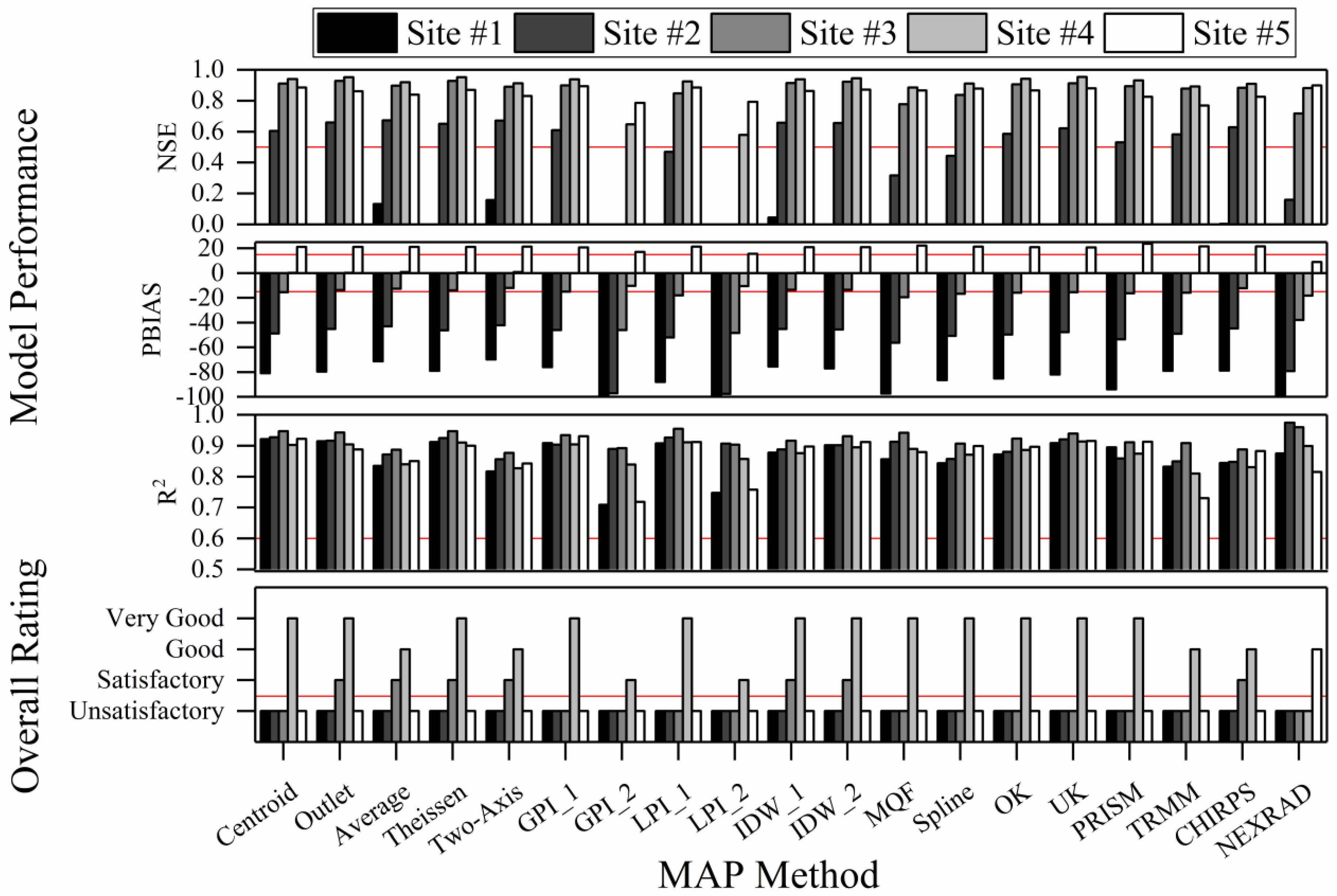
3.2.1. Uncalibrated Model Performance
3.2.2. Calibrated Model Performance
4. Conclusions
Acknowledgments
Author Contributions
Conflicts of Interest
References
- De Amorim Borges, P.; Franke, J.; da Anunciação, Y.M.T.; Weiss, H.; Bernhofer, C. Comparison of spatial interpolation methods for the estimation of precipitation distribution in Distrito Federal, Brazil. Theor. Appl. Climatol. 2016, 123, 335–348. [Google Scholar] [CrossRef] [Scilit]
- Militino, A.F.; Ugarte, M.D.; Goicoa, T.; Genton, M. Interpolation of daily rainfall using spatiotemporal models and clustering. Int. J. Climatol. 2015, 35, 1453–1464. [Google Scholar] [CrossRef] [Scilit]
- Nicótina, L.; Alessi Celegon, E.; Rinaldo, A.; Marani, M. On the impact of rainfall patterns on the hydrologic response. Water Resour. Res. 2008, 44. [Google Scholar] [CrossRef] [Scilit]
- Masih, I.; Maskey, S.; Uhlenbrook, S.; Smakhtin, V. Assessing the impact of areal precipitation input on streamflow simulations using the SWAT model. J. Am. Water Resour. Assoc. 2011, 47, 179–195. [Google Scholar] [CrossRef] [Scilit]
- Gassman, P.W.; Reyes, M.R.; Green, C.H.; Arnold, J.G. The Soil and Water Assessment Tool: Historical development, applications, and future research directions. Trans. ASABE 2007, 50, 1211–1250. [Google Scholar] [CrossRef] [Scilit]
- Neitsch, S.L.; Arnold, J.G.; Kiniry, J.R.; Williams, J.R. Soil and Water Assessment Tool Theoretical Documentation Version 2009; Texas Water Resources Institute Technical Report No. 406; Texas Water Resources Institute: College Station, TX, USA, 2009. [Google Scholar]
- Thiessen, A.H. Precipitation averages for large areas. Mon. Weather Rev. 1911, 39, 1082–1089. [Google Scholar] [CrossRef] [Scilit]
- Bethlahmy, N. The two-axis method: A new method to calculate average precipitation over basin. Hydrol. Sci. J. 1976, 21, 379–385. [Google Scholar] [CrossRef] [Scilit]
- Wang, S.; Huang, G.H.; Lin, Q.G.; Li, Z.; Zhang, H.; Fan, Y.R. Comparison of interpolation methods for estimating spatial distribution of precipitation in Ontario, Canada. Int. J. Climatol. 2014, 34, 3745–3751. [Google Scholar] [CrossRef] [Scilit]
- Johnston, K.; Ver Hoef, J.M.; Krivoruchko, K.; Lucas, N. Using ArcGIS Geostatistical Analyst; ESRI Press: Redlands, CA, USA, 2001; Volume 380. [Google Scholar]
- Luo, W.; Taylor, M.C.; Parker, S.R. A comparison of spatial interpolation methods to estimate continuous wind speed surfaces using irregularly distributed data from England and Wales. Int. J. Climatol. 2008, 28, 947–959. [Google Scholar] [CrossRef] [Scilit]
- Dawson, C.W.; Wilby, R.L. Hydrological modelling using artificial neural networks. Prog. Phys. Geogr. 2001, 25, 80–108. [Google Scholar] [CrossRef] [Scilit]
- Govindaraju, R. Artificial neural networks in hydrology. I: Preliminary concepts. J. Hydrol. Eng. 2000, 5, 115–123. [Google Scholar]
- Govindaraju, R. Artificial neural networks in hydrology. II: Hydrologic applications. J. Hydrol. Eng. 2000, 5, 124–137. [Google Scholar]
- Daly, C.; Neilson, R.P.; Phillips, D.L. A statistical-topographic model for mapping climatological precipitation over mountainous terrain. J. Appl. Meteorol. 1994, 33, 140–158. [Google Scholar] [CrossRef] [Scilit]
- Daly, C.; Smith, J.I.; Olson, K.V. Mapping atmospheric moisture climatologies across the conterminous United States. PLoS ONE 2015, 10, e0141140. [Google Scholar]
- Szcześniak, M.; Piniewski, M. Improvement of hydrological simulations by applying daily precipitation interpolation schemes in meso-scale catchments. Water 2015, 7, 747–779. [Google Scholar] [CrossRef] [Scilit]
- Krysanova, V.; Srinivasan, R. Assessment of climate and land use change impacts with SWAT. Reg. Environ. Chang. 2015, 15, 431. [Google Scholar] [CrossRef] [Scilit]
- Borah, D.K.; Arnold, J.G.; Bera, M.; Krug, E.C.; Liang, X.Z. Storm event and continuous hydrologic modeling for comprehensive and efficient watershed simulations. J. Hydrol. Eng. 2007, 12, 605–616. [Google Scholar] [CrossRef] [Scilit]
- de Almeida Bressiani, D.; Gassman, P.W.; Fernandes, J.G.; Garbossa, L.H.P.; Srinivasan, R.; Bonumá, N.B.; Mendiondo, E.M. Review of soil and water assessment tool (SWAT) applications in Brazil: Challenges and prospects. Int. J. Agric. Biol. Eng. 2015, 8, 9. [Google Scholar]
- Anjum, M.N.; Ding, Y.; Shangguan, D.; Tahir, A.A.; Iqbal, M.; Adnan, M. Comparison of two successive versions 6 and 7 of TMPA satellite precipitation products with rain gauge data over Swat Watershed, Hindukush Mountains, Pakistan. Atmos. Sci. Lett. 2016, 17, 270–279. [Google Scholar] [CrossRef] [Scilit]
- Yang, Y.; Wang, G.; Wang, L.; Yu, J.; Xu, Z. Evaluation of gridded precipitation data for driving swat model in area upstream of three gorges reservoir. PLoS ONE 2014, 9, e112725. [Google Scholar]
- Yu, M.; Chen, X.; Li, L.; Bao, A.; De la Paix, M.J. Streamflow simulation by SWAT using different precipitation sources in large arid basins with scarce rain gauges. Water Resour. Manag. 2011, 25, 2669–2681. [Google Scholar] [CrossRef] [Scilit]
- Zhu, H.; Li, Y.; Liu, Z.; Shi, X.; Fu, B.; Xing, Z. Using SWAT to simulate streamflow in Huifa River basin with ground and Fengyun precipitation data. J. Hydroinform. 2015, 17, 834–844. [Google Scholar] [CrossRef] [Scilit]
- Strauch, M.; Bernhofer, C.; Koide, S.; Volk, M.; Lorz, C.; Makeschin, F. Using precipitation data ensemble for uncertainty analysis in SWAT streamflow simulation. J. Hydrol. 2012, 414, 413–424. [Google Scholar] [CrossRef] [Scilit]
- Tuo, Y.; Duan, Z.; Disse, M.; Chiogna, G. Evaluation of precipitation input for SWAT modeling in Alpine catchment: A case study in the Adige river basin (Italy). Sci. Total Environ. 2016, 573, 66–82. [Google Scholar] [CrossRef] [Scilit] [PubMed]
- Ly, S.; Charles, C.; Degré, A. Different methods for spatial interpolation of rainfall data for operational hydrology and hydrological modeling at watershed scale: A review. Biotechnol. Agron. Soc. Environ. 2013, 17, 392–406. [Google Scholar]
- Zhang, X.; Srinivasan, R. GIS-Based Spatial Precipitation Estimation: A Comparison of Geostatistical Approaches1. J. Am. Water Resour. Assoc. 2009, 45, 894–906. [Google Scholar] [CrossRef] [Scilit]
- Goovaerts, P. Geostatistical approaches for incorporating elevation into the spatial interpolation of rainfall. J. Hydrol. 2000, 228, 113–129. [Google Scholar] [CrossRef] [Scilit]
- Hartkamp, A.D.; de Beurs, K.; Stein, A.; White, J.W. Interpolation Techniques for Climate Variables NRG-GIS Series 99–01; CIMMYT: Méx., Mexico, 1999. [Google Scholar]
- Tabios, G.Q.; Salas, J.D. A comparative analysis of techniques for spatial interpolation of precipitation. Water Resour. Bull. 1985, 21, 365–380. [Google Scholar] [CrossRef] [Scilit]
- Hubbart, J.A.; Holmes, J.; Bowman, G. Integrating science based decision making and TMDL allocations in urbanizing watersheds. Watershed Sci. Bull. 2010, 1, 19–24. [Google Scholar]
- Hubbart, J.A.; Kellner, E.; Lynne, H.; Lupo, A.R.; Market, P.S.; Guinan, P.E.; Stephan, K.; Fox, N.I.; Svoma, B. Localized climate and surface energy flux alterations across an urban gradient in the central US. Energies 2014, 7, 1770–1791. [Google Scholar] [CrossRef] [Scilit]
- Kellner, E.; Hubbart, J.A. Application of the experimental watershed approach to advance urban watershed precipitation/discharge understanding. Urban Ecosyst. 2016. [Google Scholar] [CrossRef] [Scilit]
- Zeiger, S.J.; Hubbart, J.A. A SWAT model validation of nested-scale contemporaneous stream flow, suspended sediment and nutrients from a multiple-land-use watershed of the central USA. Sci. Total Environ. 2016, 572, 232–243. [Google Scholar] [CrossRef] [Scilit] [PubMed]
- Zeiger, S.J.; Hubbart, J.A. Quantifying suspended sediment flux in a mixed-land use urbanizing watershed using a nested-scale study design. Sci. Total Environ. 2016, 542, 315–323. [Google Scholar] [CrossRef] [Scilit] [PubMed]
- Zeiger, S.J.; Hubbart, J.A. Nested-Scale nutrient yields from a mixed-land-use urbanizing watershed. Hydrol. Process. 2015, 30, 1475–1490. [Google Scholar] [CrossRef] [Scilit]
- Zeiger, S.J.; Hubbart, J.A.; Anderson, S.H.; Stambaugh, M.L. Quantifying and modeling urban stream temperature: A central US watershed study. Hydrol. Process. 2015, 30, 503–514. [Google Scholar]
- Sauer, V.B.; Turnipseed, D.P. Stage Measurement at Gaging Stations: US Geological Survey Techniques and Methods book 3, Chap. A7. 2010; 45p. Available online: http://pubs.usgs.gov/tm/tm3-a7 (accessed on 1 October 2016).
- Dottori, F.; Martina, M.L.V.; Todini, E. A dynamic rating curve approach to indirect discharge measurement. Hydrol. Earth Syst. Sci. 2009, 13, 847. [Google Scholar] [CrossRef] [Scilit]
- Kochendorfer, J.; Rasmussen, R.; Wolff, M.; Baker, B.; Hall, M.E.; Meyers, T.; Landolt, S.; Jachcik, A.; Isaksen, K.; Brækkan, R.; et al. The quantification and correction of wind-induced precipitation measurement errors. Hydrol. Earth Syst. Sci. 2017, 21, 1973–1989. [Google Scholar] [CrossRef] [Scilit]
- Dingman, S.L. Physical Hydrology, Chapter 4: Precipitation; Waveland Press: Salem, WI, USA, 2002; pp. 159–209. [Google Scholar]
- Siriwardena, L.; Finlayson, B.L.; McMahon, T.A. The impact of land use change on catchment hydrology in large catchments: The Comet River, Central Queensland, Australia. J. Hydrol. 2006, 326, 199–214. [Google Scholar] [CrossRef] [Scilit]
- Wagner, P.D.; Fiener, P.; Wilken, F.; Kumar, S.; Schneider, K. Comparison and evaluation of spatial interpolation schemes for daily rainfall in data scarce regions. J. Hydrol. 2012, 464, 388–400. [Google Scholar] [CrossRef] [Scilit]
- Suhaila, J.; Sayang, M.D.; Jemain, A.A. Revised spatial weighting methods for estimation of missing rainfall data. Asia-Pac. J. Atmos. Sci. 2008, 44, 93–104. [Google Scholar]
- Moriasi, D.N.; Gitau, M.W.; Pai, N.; Daggupati, P. Hydrologic and water quality models: Performance measures and evaluation criteria. Trans. ASABE 2015, 58, 1763–1785. [Google Scholar] [CrossRef] [Scilit]
- Moriasi, D.N.; Arnold, J.G.; Van Liew, M.W.; Bingner, R.L.; Harmel, R.D.; Veith, T.L. Model evaluation guidelines for systematic quantification of accuracy in watershed simulations. Trans. ASABE 2007, 50, 885–900. [Google Scholar] [CrossRef] [Scilit]
- PRISM Climate Data. Available online: http://www.prism.oregonstate.edu/ (accessed on 1 October 2016).
- Giovanni. Available online: https://giovanni.sci.gsfc.nasa.gov/giovanni/ (accessed on 1 October 2016).
- ClimateSERV. Available online: https://climateserv.servirglobal.net/ (accessed on 1 October 2016).
- National Weather Service Advanced Hydrologic Prediction Service. Available online: https://water.weather.gov/precip/ (accessed on 1 October 2016).
- Arnold, J.G.; Moriasi, D.N.; Gassman, P.W.; Abbaspour, K.C.; White, M.J.; Srinivasan, R.; Santhi, C.; Harmel, R.D.; van Griensven, A.; Van Liew, M.W.; et al. SWAT: Model use, calibration, and validation. Trans. ASABE 2012, 55, 1491–1508. [Google Scholar] [CrossRef] [Scilit]
- Engel, B.; Storm, D.; White, M.; Arnold, J.G. A hydrologic/water quality model application protocol. J. Am. Water Resour. Assoc. 2007, 43, 1223–1236. [Google Scholar] [CrossRef] [Scilit]
- Srinivasan, R.; Zhang, X.; Arnold, J. SWAT Ungauged: Hydrological budget and crop yield predictions in the upper Mississippi river basin. Trans. ASABE 2010, 53, 1533–1546. [Google Scholar] [CrossRef] [Scilit]
- Baffaut, C.; Sadler, E.J.; Ghidey, F. Long-term agroecosystem research in the Central Mississippi River Basin: Goodwater Creek Experimental Watershed flow data. J. Environ. Qual. 2015, 44, 17–26. [Google Scholar] [CrossRef] [Scilit] [PubMed]
- Gali, R.K.; Douglas-Mankin, K.R.; Li, X.; Xu, T. Assessing NEXRAD P3 data effects on stream-flow simulation using SWAT model in an agricultural watershed. J. Hydrol. Eng. 2012, 17, 1245–1254. [Google Scholar] [CrossRef] [Scilit]
- Sexton, A.M.; Sadeghi, A.M.; Zhang, X.; Srinivasan, R.; Shirmohammadi, A. Using NEXRAD and rain gauge precipitation data for hydrologic calibration of SWAT in a northeastern watershed. Trans. ASABE 2010, 53, 1501–1510. [Google Scholar] [CrossRef] [Scilit]
- Tobin, K.J.; Bennett, M.E. Using SWAT to model streamflow in two river basins with ground and satellite precipitation data1. J. Am. Water Resour. Assoc. 2009, 45, 253–271. [Google Scholar] [CrossRef] [Scilit]
- Simpson, M.; Hubbart, J.A.; Fox, N.I. Ground truthed performance of single- and dual-polarized radar rain rates at large ranges. Hydrol. Process. 2016, 30, 3692–3703. [Google Scholar] [CrossRef] [Scilit]



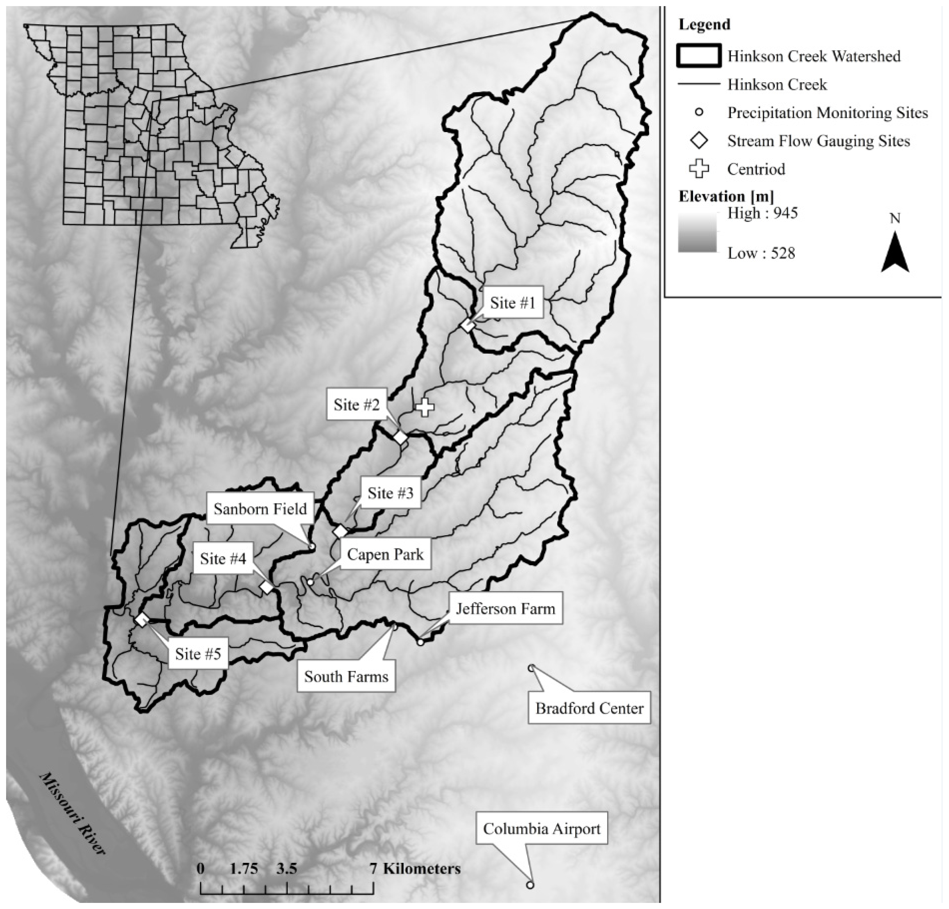
| Monitoring Site | Latitude | Longitude | Distance to Cent. (km) | Start Date | End Date |
|---|---|---|---|---|---|
| Site #1 | 39.022652° | −92.246678° | 3.803 | 1 February 2009 | 26 July 2015 |
| Site #2 | 38.981900° | −92.278671° | 1.644 | 6 February 2009 | 26 July 2015 |
| Site #3 | 38.947583° | −92.307016° | 6.053 | 8 February 2009 | 10 August 2015 |
| Site #4 | 38.927767° | −92.341505° | 9.615 | 1 March 2009 | 30 September 2015 |
| Site #5 | 38.916072° | −92.399946° | 14.34 | 13 February 2009 | 17 August 2015 |
| Sanborn Field † | 38.942301° | −92.320395° | 7.256 | 1 October 2008 | 30 September 2015 |
| Capen Park | 38.929237° | −92.321297° | 8.470 | 1 January 2011 | 30 September 2015 |
| South Farm † | 38.912626° | −92.282326° | 8.993 | 1 October 2008 | 30 September 2015 |
| Jefferson Farm † | 38.906992° | −92.269976° | 9.524 | 1 October 2008 | 30 September 2015 |
| Bradford Center | 38.897236° | −92.218070° | 11.42 | 25 April 2009 | 30 September 2015 |
| Columbia Airport | 38.818127° | −92.219672° | 19.82 | 1 October 2008 | 30 September 2015 |
| Technique | MAP Method |
|---|---|
| Proximate gauge (PG) | Nearest centroid (Centoid) |
| Sub-basin outlet (Outlet) | |
| Direct-weighted average (AVE) | Arithmetic average (Average) |
| Thiessen polygons (Thiessen) | |
| Two-axis | |
| Surface-fitted (SF) | 1st order global polynomial interpolation (GPI_1) |
| 2nd order global polynomial interpolation (GPI_2) | |
| 1st order local polynomial interpolation (LPI_1) | |
| 2nd order local polynomial interpolation (LPI_2) | |
| 1st order inverse distance weighted (IDW_1) | |
| 2nd order inverse distance weighted (IDW_2) | |
| Spline tension (Spline) | |
| Multiquadric formula (MQF) | |
| Ordinary kriging (OK) | |
| Universal kriging (UK) | |
| Remotely sensed (RS) | Parameter-elevation Regressions on Independent Slopes Model (PRISM) |
| Tropical Rainfall Measuring Mission (TRMM) | |
| Climate Hazards Group InfraRed Precipitation with Station data (CHIRPS) | |
| Next Generation Radar Data (NEXRAD) |
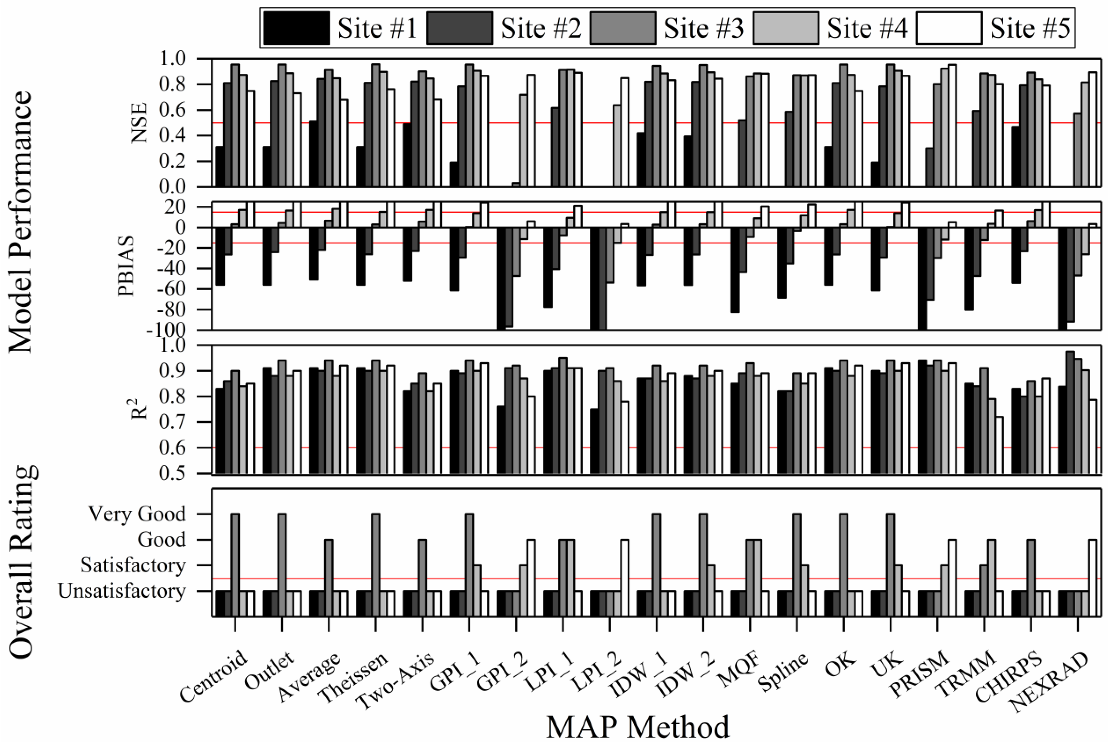
| Performance Rating | NSE | PBIAS (%) | R2 |
|---|---|---|---|
| Very good | x > 0.8 | |x| < 5 | x > 0.85 |
| Good | 0.7 < x ≤ 0.8 | 5 ≤ |x| < 10 | 0.75 < x ≤ 0.85 |
| Satisfactory | 0.50 < x ≤ 0.7 | 10 ≤ |x| < 15 | 0.60 < x ≤ 0.75 |
| Unsatisfactory | x ≤ 0.50 | |x| ≥ 15 | x ≥ 0.60 |
| Monitoring Site | 2009 | 2010 | 2011 | 2012 | 2013 | 2014 | 2015 |
|---|---|---|---|---|---|---|---|
| Site#1 | 992 | 1646 | 794 | 660 | 1055 | 890 | 1236 |
| Site#2 | 958 | 1624 | 757 | 703 | 1077 | 946 | 1159 |
| Site#3 | 1118 | 1610 | 796 | 784 | 1034 | 917 | 1156 |
| Site#4 | 1042 | 1584 | 811 | 746 | 1054 | 915 | 1100 |
| Site#5 | 1067 | 1602 | 770 | 755 | 996 | 930 | 1091 |
| Sanborn Field † | 1088 | 1651 | 762 | 739 | 960 | 867 | 1053 |
| Capen Park | 1052 | 1463 | 795 | 738 | 976 | 891 | 1045 |
| South Farm † | 1157 | 1550 | 755 | 752 | 947 | 917 | 1093 |
| Jefferson Farm † | 1062 | 1371 | 640 | 697 | 914 | 906 | 1076 |
| Bradford | 1036 | 1412 | 689 | 733 | 916 | 883 | 1093 |
| Columbia Airport | 1018 | 1453 | 891 | 868 | 1047 | 926 | 1189 |
| All-Site Average | 1054 | 1542 | 769 | 743 | 998 | 908 | 1117 |
| Technique | Method | 2009 | 2010 | 2011 | 2012 | 2013 | 2014 | 2015 |
|---|---|---|---|---|---|---|---|---|
| Proximate Gauge | Centroid | 1035 | 1613 | 786 | 730 | 1043 | 920 | 1149 |
| Outlet | 988 | 1625 | 783 | 694 | 1064 | 917 | 1178 | |
| Direct- weighted Average | Average † | 1053 | 1543 | 769 | 743 | 998 | 908 | 1117 |
| Thiessen | 1025 | 1614 | 782 | 713 | 1044 | 914 | 1170 | |
| Two-axis | 1050 | 1525 | 778 | 757 | 998 | 910 | 1123 | |
| Surface-fitted | GPI_1 | 1031 | 1615 | 775 | 702 | 1042 | 918 | 1172 |
| GPI_2 | 1161 | 1767 | 802 | 738 | 1044 | 932 | 1193 | |
| LPI_1 | 1041 | 1646 | 784 | 709 | 1048 | 915 | 1186 | |
| LPI_2 | 1173 | 1791 | 812 | 747 | 1045 | 914 | 1200 | |
| IDW_1 | 1042 | 1587 | 780 | 734 | 1028 | 917 | 1148 | |
| IDW_2 | 1033 | 1604 | 780 | 723 | 1039 | 917 | 1158 | |
| Spline | 1010 | 1655 | 781 | 708 | 1044 | 924 | 1180 | |
| MQF | 1038 | 1662 | 783 | 717 | 1035 | 920 | 1184 | |
| OK | 1022 | 1612 | 781 | 719 | 1038 | 923 | 1162 | |
| UK | 1031 | 1616 | 775 | 702 | 1043 | 918 | 1172 | |
| Remotely sensed | PRISM | 1197 | 1720 | 918 | 853 | 1140 | 1073 | 1319 |
| TRMM | 1162 | 1593 | 968 | 940 | 1149 | 942 | 1203 | |
| CHIRPS | 1051 | 1595 | 911 | 828 | 1105 | 1034 | 1252 | |
| NEXRAD | 1236 | 1759 | 1027 | 892 | 1100 | 1068 | 1260 |
| Technique | Method | RMSE | MAE | PBIAS |
|---|---|---|---|---|
| Surface-fitted | GPI_1 | 68.2 | 55.5 | −4.6 |
| GPI_2 | 69.2 | 57.0 | −5.1 | |
| LPI_1 | 63.2 | 51.8 | −4.5 | |
| LPI_2 | 68.1 | 55.8 | −5.1 | |
| IDW_1 | 66.9 | 54.2 | −4.7 | |
| IDW_2 | 67.7 | 54.7 | −5.1 | |
| MQF | 65.5 | 53.3 | −5.0 | |
| Spline | 64.6 | 53.4 | −5.0 | |
| OK | 63.5 | 52.2 | −4.6 | |
| UK | 68.2 | 55.4 | −4.6 | |
| Remotely sensed | PRISM | 148.3 | 139.2 | −13.8 |
| TRMM | 148.7 | 121.9 | −11.4 | |
| CHIRPS | 123.5 | 107.7 | −9.8 | |
| NEXRAD | 166.8 | 152.5 | −14.7 |
| Overall Rank | Technique | Method | PBIAS (%) | Daily | Monthly | Annual | |||
|---|---|---|---|---|---|---|---|---|---|
| NSE | R2 | NSE | R2 | NSE | R2 | ||||
| 1 | RS | PRISM | −11.6 | 0.16 | 0.26 | 0.71 | 0.72 | 0.92 | 0.90 |
| 2 | SF | IDW_2 | 14.9 | 0.40 | 0.45 | 0.67 | 0.69 | 0.89 | 0.88 |
| 3 | SF | IDW_1 | 15.1 | 0.41 | 0.45 | 0.68 | 0.70 | 0.89 | 0.86 |
| 4 | SF | LPI_1 | 9.40 | 0.26 | 0.41 | 0.58 | 0.61 | 0.91 | 0.91 |
| 5 | PG | Outlet | 16.4 | 0.41 | 0.45 | 0.69 | 0.71 | 0.89 | 0.88 |
| 6 | SF | OK | 13.9 | 0.39 | 0.45 | 0.63 | 0.65 | 0.87 | 0.88 |
| 7 | SF | GPI_1 | 13.9 | 0.33 | 0.43 | 0.63 | 0.64 | 0.91 | 0.90 |
| 8 | SF | UK | 13.9 | 0.33 | 0.43 | 0.63 | 0.64 | 0.91 | 0.90 |
| 9 | SF | MQF | 8.9 | 0.27 | 0.42 | 0.57 | 0.60 | 0.89 | 0.88 |
| 10 | SF | Spline | 11.8 | 0.36 | 0.44 | 0.63 | 0.64 | 0.87 | 0.85 |
| 11 | AVE | Thiessen | 15.3 | 0.36 | 0.43 | 0.63 | 0.65 | 0.90 | 0.90 |
| 12 | RS | TRMM | 3.90 | 0.26 | 0.31 | 0.53 | 0.53 | 0.87 | 0.79 |
| 13 | AVE | Two-Axis | 17.0 | 0.42 | 0.44 | 0.65 | 0.69 | 0.85 | 0.82 |
| 14 | AVE | Average | 18.2 | 0.42 | 0.45 | 0.65 | 0.69 | 0.85 | 0.84 |
| 15 | PG | Centroid | 17.2 | 0.36 | 0.44 | 0.63 | 0.65 | 0.87 | 0.88 |
| 16 | SF | GPI_2 | −11.4 | −0.24 | 0.33 | 0.14 | 0.48 | 0.72 | 0.87 |
| 17 | SF | LPI_2 | −15.1 | −0.33 | 0.33 | 0.02 | 0.47 | 0.64 | 0.86 |
| 18 | RS | NEXRAD | −25.5 | 0.13 | 0.25 | 0.59 | 0.63 | 0.82 | 0.90 |
| 19 | RS | CHIRPS | 17.1 | 0.26 | 0.27 | 0.49 | 0.52 | 0.84 | 0.80 |
| Overall Rank | Technique | Method | PBIAS (%) | Daily | Monthly | Annual | |||
|---|---|---|---|---|---|---|---|---|---|
| NSE | R2 | NSE | R2 | NSE | R2 | ||||
| 1 | SF | IDW_2 | 0.00 | 0.41 | 0.48 | 0.74 | 0.74 | 0.95 | 0.89 |
| 2 | SF | IDW_1 | 0.16 | 0.40 | 0.47 | 0.77 | 0.77 | 0.94 | 0.88 |
| 3 | SF | UK | 0.00 | 0.18 | 0.41 | 0.67 | 0.68 | 0.95 | 0.91 |
| 4 | SF | GPI_1 | 0.02 | 0.34 | 0.49 | 0.65 | 0.70 | 0.94 | 0.90 |
| 5 | RS | PRISM | 0.00 | 0.36 | 0.38 | 0.68 | 0.69 | 0.93 | 0.87 |
| 6 | PG | Centroid | 0.16 | 0.36 | 0.47 | 0.69 | 0.70 | 0.94 | 0.90 |
| 7 | PG | Outlet | 0.18 | 0.31 | 0.44 | 0.75 | 0.75 | 0.95 | 0.90 |
| 8 | SF | OK | 0.02 | 0.30 | 0.44 | 0.71 | 0.71 | 0.94 | 0.89 |
| 9 | AVE | Average | 0.77 | 0.41 | 0.48 | 0.77 | 0.77 | 0.92 | 0.84 |
| 10 | SF | Spline | 0.01 | 0.35 | 0.46 | 0.68 | 0.69 | 0.91 | 0.87 |
| 11 | SF | LPI_1 | 0.01 | 0.29 | 0.45 | 0.57 | 0.65 | 0.93 | 0.91 |
| 12 | AVE | Thiessen | 0.42 | 0.36 | 0.46 | 0.68 | 0.69 | 0.95 | 0.91 |
| 13 | AVE | Two-Axis | 0.91 | 0.37 | 0.47 | 0.76 | 0.76 | 0.91 | 0.83 |
| 14 | SF | MQF | 0.01 | 0.27 | 0.42 | 0.57 | 0.62 | 0.89 | 0.89 |
| 15 | RS | NEXRAD | −18.2 | 0.38 | 0.40 | 0.71 | 0.75 | 0.88 | 0.90 |
| 16 | RS | TRMM | −0.01 | 0.24 | 0.32 | 0.58 | 0.58 | 0.89 | 0.81 |
| 17 | RS | CHIRPS | 0.03 | 0.26 | 0.29 | 0.59 | 0.60 | 0.91 | 0.83 |
| 18 | SF | GPI_2 | −10.4 | 0.12 | 0.35 | 0.18 | 0.43 | 0.65 | 0.84 |
| 19 | SF | LPI_2 | −10.5 | −0.02 | 0.38 | 0.23 | 0.47 | 0.58 | 0.86 |
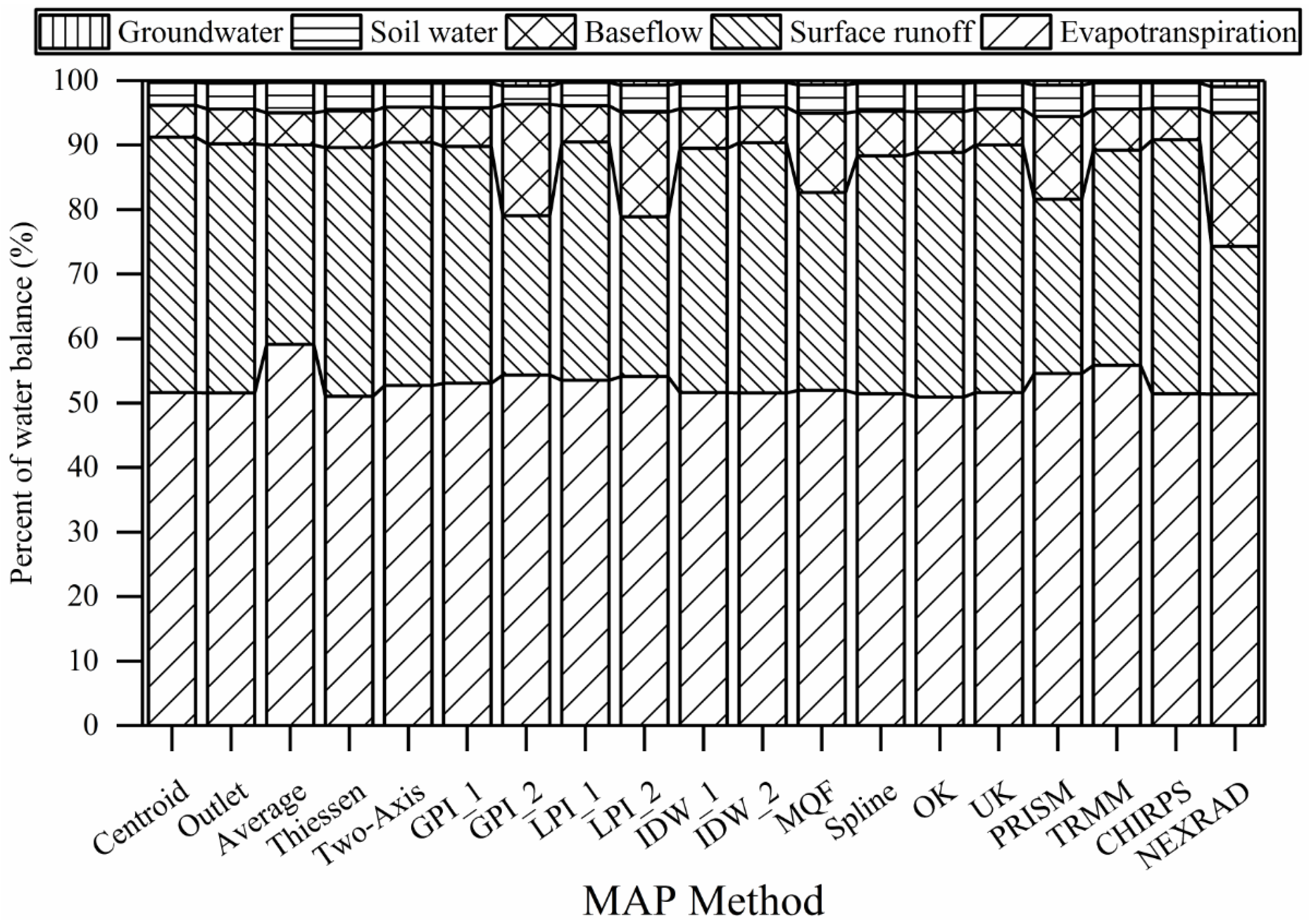
| Technique | MAP Method | Precip. | ET | Surface Runoff (mm) (%) | Baseflow | Soil Water | Ground Water |
|---|---|---|---|---|---|---|---|
| Proximate gauge | Centroid | 1039 | 537 (52) | 412 (40) | 51 (5) | 37 (4) | 3 (0) |
| Outlet | 1036 | 536 (52) | 402 (39) | 56 (5) | 42 (4) | 4 (0) | |
| Direct-weighted average | Average | 1019 | 604 (59) | 316 (31) | 51 (5) | 48 (4) | 3 (0) |
| Thiessen | 1037 | 532 (51) | 402 (39) | 59 (6) | 45 (4) | 4 (0) | |
| Two-Axis | 1020 | 540 (53) | 386 (38) | 56 (5) | 38 (3) | 4 (0) | |
| Surface-fitting | GPI_1 | 1036 | 552 (53) | 382 (37) | 62 (6) | 40 (3) | 4 (0) |
| GPI_2 | 1091 | 597 (55) | 272 (25) | 190 (17) | 31 (2) | 9 (1) | |
| LPI_1 | 1047 | 562 (54) | 388 (37) | 59 (6) | 38 (3) | 3 (0) | |
| LPI_2 | 1097 | 598 (55) | 274 (25) | 179 (16) | 46 (3) | 8 (1) | |
| IDW_1 | 1034 | 536 (52) | 393 (38) | 64 (6) | 41 (4) | 4 (0) | |
| IDW_2 | 1036 | 536 (52) | 404 (39) | 57 (6) | 40 (3) | 3 (0) | |
| MQF | 1043 | 546 (52) | 322 (31) | 129 (12) | 46 (4) | 7 (1) | |
| Spline | 1048 | 542 (52) | 388 (37) | 73 (7) | 46 (4) | 4 (0) | |
| OK | 1037 | 530 (51) | 395 (38) | 66 (6) | 46 (4) | 4 (0) | |
| UK | 1037 | 537 (52) | 399 (38) | 58 (6) | 43 (4) | 3 (0) | |
| Remotely sensed | PRISM | 1174 | 645 (55) | 320 (27) | 151 (13) | 58 (4) | 8 (1) |
| TRMM | 1137 | 637 (56) | 380 (33) | 73 (6) | 46 (4) | 4 (0) | |
| CHIRPS | 1111 | 574 (52) | 440 (40) | 54 (5) | 44 (4) | 4 (0) | |
| NEXRAD | 1192 | 618 (52) | 275 (23) | 249 (21) | 49 (3) | 11 (1) |
© 2017 by the authors. Licensee MDPI, Basel, Switzerland. This article is an open access article distributed under the terms and conditions of the Creative Commons Attribution (CC BY) license (http://creativecommons.org/licenses/by/4.0/).
Share and Cite
Zeiger, S.; Hubbart, J. An Assessment of Mean Areal Precipitation Methods on Simulated Stream Flow: A SWAT Model Performance Assessment. Water 2017, 9, 459. https://doi.org/10.3390/w9070459
Zeiger S, Hubbart J. An Assessment of Mean Areal Precipitation Methods on Simulated Stream Flow: A SWAT Model Performance Assessment. Water. 2017; 9(7):459. https://doi.org/10.3390/w9070459
Chicago/Turabian StyleZeiger, Sean, and Jason Hubbart. 2017. "An Assessment of Mean Areal Precipitation Methods on Simulated Stream Flow: A SWAT Model Performance Assessment" Water 9, no. 7: 459. https://doi.org/10.3390/w9070459
APA StyleZeiger, S., & Hubbart, J. (2017). An Assessment of Mean Areal Precipitation Methods on Simulated Stream Flow: A SWAT Model Performance Assessment. Water, 9(7), 459. https://doi.org/10.3390/w9070459