Abstract
Water quality assessments are essential for providing information regarding integrated water resource management processes. This study presents the results of a spatial and seasonal surface water quality assessment of the Burío river sub-catchment in Costa Rica. Fourteen sample campaigns were conducted at eight sample sites between 2005 and 2010. Seasonal variations were evaluated using linear mixed-effects models where dissolved oxygen, total solids, and nitrate showed significant differences between dry and wet seasons (p < 0.05). Cluster analysis identified three clusters at the top, middle, and bottom of the catchment that were consistent with land use patterns, and principal component analysis identified the main parameters that were affecting 84% of the total variance in water quality (biochemical oxygen demand, dissolved oxygen, total phosphate, and nitrate). The National Sanitation Foundation Water Quality Index (NSF-WQI) results indicated the majority of the river consisted of mainly “medium” water quality, although “bad” and “good” water quality results were identified depending on sample site and season. This methodological approach provides a useful monitoring technique for local governments that can be used for further remediation strategies.
1. Introduction
Surface water quality assessments are essential in providing sustainable and efficient water resource management [1]. Although surface water can become contaminated through natural processes [2], it is through anthropogenic changes in land cover (LC) and land use (LU) which tend to cause the greatest levels of pollution [3]. This is most apparent in developing countries where monitoring and remediation programs are rare, but deterioration of water quality is strongly associated with increased point and diffuse pollution, caused from rapidly expanding urban, industrial, and agricultural activities [4,5]. Furthermore, in many developing countries, these anthropogenic activities tend to outpace the institutional and infrastructure capacities required to manage increased levels of pollution [6]. Surface water quality assessments—particularly in these countries—are therefore essential for policymakers and watershed managers in understanding the main causes of pollution and providing a first step towards remediation strategies [7,8].
Although there are practical guidelines for the implementation of these assessments, local conditions such as land use, national regulations, geography, and geomorphology, for example, should also be considered [9]. The assessments usually involve the collection and analyses of: biological (e.g., Escherichia coli) [10]; chemical (e.g., dissolved oxygen) [11]; physical (e.g., water temperature); and radiological (e.g., radium) [12] parameters, obtained at different monitoring times (temporal changes), and at multiple sampling sites (spatial changes) [13,14,15].
Monitoring networks, ranging from fully automatic to manual [16], can deliver reliable information quickly in a sustainable and cost-effective way when data are assessed accurately [17]. Furthermore, although several analytical methods have been used to interpret water quality results [9,18], statistical techniques such as mixed-effects models [19,20] and multivariate analyses such as: cluster analysis (CA); factor analysis (FA); principal component analysis (PCA); and discriminant analysis (DA) [21,22,23] provide a reliable method for identifying the main parameters which influence water quality—spatially and temporally—within a particular catchment. However, in order to compare water quality across different catchments, various water quality indices (WQIs) have been developed to provide an overall water quality score, reflecting the aggregated influence of a selected group of water quality parameters, which are usually compared to regulatory standards [24].
One of the main sources of pollution in surface waters and causes of water-borne diseases in Latin America and the Caribbean region is from untreated sewage from urban areas [25]. In particular, only 49% of households have connections to conventional sewage systems, 30% only have in situ sanitation systems (i.e., septic tanks and latrines), whilst 21% have no wastewater or sewage disposal [26]. Overall, only 14% of the collected sewage receives any kind of treatment [27]. In Costa Rica, although 99% of the population have access to domestic water supply, only 82% have access to consistent potable drinking water, and this percentage is far less in rural areas. Furthermore, only 3% of sewage is treated before being discharged into the environment [28]. The majority of the population relies on groundwater for drinking water, yet studies indicate that nitrate concentrations in groundwater are likely to exceed recommended values due to inadequate waste disposal from urban areas and coffee fertilization practices [29].
This study presents results of one of the few monitoring programs to examine the spatial and seasonal variation in surface water quality in Costa Rica, specifically of the Burío river sub-catchment. The sub-catchment forms part of the upper reaches of the Grande de Tárcoles catchment which underlies the largest urban area in the country and is generally considered one of the most polluted catchments in Central America [28]. The combination of methodological techniques employed in this study offer a framework for developing water monitoring programs and formulating evidence-based water resource management strategies when resources are limited. This is of particular importance in developing countries such as Costa Rica, where the institutional and regulatory capacities to monitor water bodies are often limited.
2. Materials and Methods
2.1. Study Area
The Burío river is a tributary of the Grande de Tárcoles river in Costa Rica that flows from the Central Valley to the Pacific Ocean (see Figure 1). Rivers and streams in this catchment are characterized by shallow stony channels and altered banks, where natural vegetation has been removed or replaced by exotic vegetation and by urban or rural infrastructure. Under these conditions, riparian soils are unstable, facilitating their entry and that of pollutants by runoff [18]. The Burío river is 15.6 km long and flows from largely semi-rural LC in the north-east of the sub-catchment, near the town of Los Angeles, towards more urban and industrial LU in the central and south-west beginning near the towns of Barva and Heredia. Elevation ranges from 1620 m in the north-east to 856 m in the south-west. The climate in the Central Pacific of Costa Rica is characterized by a wet season (May to October) and a dry season (December to March) with April and November regarded as transition months. Average monthly precipitation varied considerably between the wet season (386 mm) and dry season (32 mm) within the Burío river sub-catchment from 2006 to 2010 [30]. However, average monthly temperature remained constant (21 C). An average of approximately 92.7 Mg per year of organic load was legally discharged as point sources of pollution to the river, mainly from wastewater treatment plants of condos and industries from 2012 to 2014 [31].
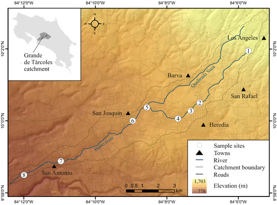
Figure 1.
The Burío river sub-catchment in the Grande de Tárcoles river catchment, Costa Rica.
The LU map illustrated in Figure 2 was generated by photo-interpretation technique using data from the Cadastral and Registral Regularization Project for Costa Rica at 1:5000 scale with a spatial resolution of approximately 2.5 m for 2005. To contrast how LU/LC has changed, a 2016 map was also made using the satellite images from Quick Bird II with a resolution of 0.6 m distributed by Digital Globe in Google Earth Pro. LC/LU were categorized into five groups: forest; arable; industry; pastoral; and urban. All spatial analyses were carried out using ArcGIS 10.4.1 (ESRI).
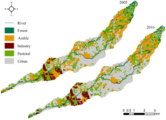
Figure 2.
Land use maps for the Burío river sub-catchment for 2005 and 2016.
2.2. Sampling Strategy and Analytical Procedure
Fourteen sample campaigns were conducted between October 2005 and December 2010, at eight selected sample sites, to assess the spatial and temporal variability in surface water quality in the Burío river. A total of 112 water samples were collected in high-density polyethylene (HDPE) and glass bottles previously washed with hydrochloric acid (HCl) 3% m/v and de-ionized water. Samples were stored at 4 C and delivered to the laboratory within 6 h of collection. All samples were analysed using the procedures of the Standard Methods for the Examination of Water and Wastewater [32]. Water temperature, dissolved oxygen (DO), and pH were measured in situ using a handheld multi-parameter probe YSI 58 for the first two parameters and a field meter HI 9025 for pH. Biochemical oxygen demand (BOD) was determined using the 5-days test with the modified Winkler method for dissolved oxygen. Nephelometry was used to analyse turbidity (HF scientific Micro 100, Fort Myers, FL, USA), and total solids (TS) were determined by gravimetry at 105 C. Total phosphate (TP) concentration was analysed spectrophotometrically by the stannous chloride method after the application of the persulfate digestion procedure (Thermo Aquamate 2000E, Mercedes Row, Cambridge, UK). Ion chromatography was used to measure nitrate concentration (Dionex 2000i/SP, Done Sunnyvale, CA, USA). Finally, faecal coliforms were determined by multiple tube fermentation technique.
2.3. Data Analyses
Prior to performing the statistical analyses below, quantification limits (QLs) were substituted by QL/2 (QL observations were less than 10%) [33]. Analysis of variance (ANOVA) was performed using linear mixed-effects model to evaluate spatial and seasonal differences for each water quality indicator [20,34]. Season and sample site were defined as fixed effects, while year and month as random effects. Evaluation of standard diagnostic graphs were performed to check the assumptions of normality and homogeneity of variance. In cases where data did not meet the assumptions, a log transformation was made and/or an independent variance function was used to correct heteroscedasticity. Least significant difference (LSD) Fisher test (p = 0.05) was employed to find mean differences among sample sites and seasons. The non-parametric Spearman’s rank correlation coefficient was used to find relationships between parameters (p < 0.05) [10,13].
Multivariate statistical techniques were used to identify different spatial patterns in water quality data. The sample sites were grouped considering similarities in water quality using the hierarchical CA with Ward method of association [35], and squared Euclidean distance as a measure of similarity. In this method, the distance between two groups depends on the sum of the sum of the squares of the analysis of variance, resulting in a dendrogram that summarises the clustering processes. PCA was carried out to identify the main parameters that explain data variation (observed groupings of the sample sites) [36,37]. PCA is a data reduction technique that transforms the original variables into a new subset of uncorrelated variables called principal components which explain the variance observed in the original data. All statistical analyses were carried out using InfoStat [38] and R [39].
Finally, to evaluate the overall water quality, the National Sanitation Foundation WQI (NSF-WQI) [40] was calculated as:
where WQI equals a number between 0 and 100 (100 indicating excellent water quality and 0 very bad); q equals the Q-value score of parameter i (a number between 0 and 100 read from the respective average quality curves developed by the NSF); w is the unit weight of parameter i (a number between 0 and 0.17 reflecting the relative importance of that parameter in the overall calculation which combined equals 1); and n is the number of parameters included in the calculation. There are nine parameters in the NSF-WQI including: DO, faecal coliform, pH, BOD, temperature change, TP, nitrate, turbidity, and TS. Water quality based on the NSF-WQI is categorized into one of five classes, including: very bad (0–25); bad (26–50); medium (51–70); good (71–90); and excellent (91–100).
3. Results and Discussion
A summary of the physical, chemical, and microbiological parameters per sample point and season are presented in Table 1. Temperature and pH were within recommended limits at each sample point during both wet and dry seasons, while turbidity, nitrate, TP, and faecal coliforms exceeded recommended values at particular points and times on the river [41]. These pollution indicators can be associated with LU/LC changes within the catchment which tend to increase point and non-point sources of pollution [42]. For example, variations in the landscape contribute to the pattern in temperature change of the river, where protected riparian zones have been reduced, resulting in increased surface water temperature. In addition, wastewater discharges consisting of surfactants from residential and commercial activities, plus the use of concrete in the border and bed of the river, tend to increase the pH value of the surface water in more urbanised-industrial zones.

Table 1.
Summary of the physiochemical and microbiological characteristics of the Burío river (mean and standard deviation).
In a decade, urban LU increased from 42.8% to 51.4%, and industrial LU from 4.2% to 5.5%; whereas forest, pastoral, and arable LU decreased from 4.3% to 3.6%, from 48.6% to 39.5%, and from 21.9% to 18.1%, respectively (Figure 2). Increased urban and industrial LU can be associated with a reduction in infiltration, increased runoff, and transport of pollutants from the sub-catchment to the river [18]. In addition, illegal wastewater discharges from non-regulated activities or discharges that do not meet the regulatory standards are constantly present in the whole sub-catchment. In the same way, the lack of sanitation system could explain the high concentration of faecal coliforms that have been previously correlated with population density within some catchments in Costa Rica [43]. Moreover, according to the national legislation of Costa Rica, the Burío river does not meet the minimum water quality requirements for irrigation (Class IV) [44], yet illegal water abstractions for agriculture persist. Further studies should be conducted to assess the impact of these activities and their potential effects on human health.
Average values for each water quality parameter per season are presented in Table 2. Only DO, TS, and nitrate were significantly different between dry and wet seasons. However, average temperature, pH, turbidity, DO, and nitrate were higher in the wet season compared to the dry season. In the wet season, DO concentration was higher as the river was highly diluted, and the dilution effect decreases the concentration of organic matter while runoff increases nitrate and turbidity. Similar results were reported by Brenes and Mora [45] in the Tárcoles and Reventazón rivers, and by Herrera et al. [46] in the Virilla basin in Costa Rica. In the dry season, low river flow and an increase in industrial wastewater discharges—particularly from coffee processing plants near sample point 2—could influence higher concentrations of TS and BOD. In general, water quality did not improve in either season, as pollution levels remained high, but the higher concentration of DO in the wet season increased the rivers’ capacity to break down organic matter. Significant interactions between season and site were identified for DO (F(7, 81) = 3.66, p = 0.002), TP (F(7, 81) = 3.38, p = 0.003) and turbidity (F(7, 81) = 4.18, p = 0.001), meaning that water quality does not follow a specific trend (depending on the season) for some sample sites. The observed spatial-temporal trends suggest that there are specific conditions at each sample point that are influencing water quality, regardless of season.
Table 2.
Differences in dry and wet seasons determined through ANOVA.
Table 3 presents Spearman’s rank correlation coefficients for the water quality indicators used in this study. The statistically significant correlations were classified depending on the coefficient value, where a coefficient value of plus or minus 0.7 was considered a strong correlation, plus or minus 0.5 a moderate correlation, and plus or minus 0.3 a weak correlation [47]. A significantly strong correlation existed between nitrate and DO. Significantly moderate correlations existed between: BOD and turbidity; nitrate and temperature; nitrate and BOD; and TP and TS. Lastly, significantly weak correlations existed between: pH and temperature; DO and temperature; turbidity and DO; TS and pH; TS and DO; TS and turbidity; BOD and DO; BOD and TS; nitrate and turbidity; TP and pH; TP and DO; TP and BOD; faecal coliform and turbidity; faecal coliform and BOD; and faecal coliform and nitrate. Correlations between BOD and TS, turbidity and TP could be explained by the organic nature of the contaminants entering the river [10], while the negative correlations between DO and TS, turbidity, BOD, TP, and faecal coliform can be associated with its degradation processes, depleting DO concentration [48]. The positive relationship between DO and nitrate and the negative relationship between nitrate and BOD may suggest that the main source of nitrate is due to organic matter degradation. Deficiencies in the domestic wastewater treatment systems could be related not only to the high concentrations of faecal coliforms as discussed above, but also with the discharge of reduced forms of nitrogen that oxidize upon contact with water to generate nitrate. Natural and anthropogenic sources of TP would be present due to their correlation with BOD and TS. The Spearman’s rank correlation was also performed by season (data not shown), indicating similar results to the ANOVA test except for TP, which was statistically significant (R = 0.37, p = 0.000). This was most likely due to the high standard error in the ANOVA.
Table 3.
Spearman’s rank correlation coefficients.
CA produced three clusters at (D/D) × 100 < 50, illustrated in Figure 3. The first cluster included just one sample site (site 1), the second group consisted of five sample sites (sites 2, 3, 4, 5, and 6) and the third cluster was formed of two sample sites (sites 7 and 8). The three clusters are located in the upper, middle, and bottom of the sub-catchment, respectively. This grouping is consistent with LU/LC changes, particularly in the middle portion of the sub-catchment where anthropogenic activities such as urbanisation and industrialisation have increased, and can be related to increased levels of pollution in the water body (Table 1). Clusters 1 and 3 can be considered as less polluted in comparison to cluster 2. Cluster 1 is located in a low population area, even though agricultural activities such as arable and pastoral are present. In particular, sample site 4 (cluster 2) is situated in the middle of the sub-catchment, and recorded the highest levels of contaminants of all eight sample sites. Interestingly, water quality improved towards the bottom of the sub-catchment, as increased river discharge increased the dilution effect, and reduced the level of pollution in the river. The results of the CA indicate similarities between sample sites, providing a methodological framework for categorising a catchment, reducing the number of sample sites [22], and improving the cost and efficiency of long-term monitoring programmes.
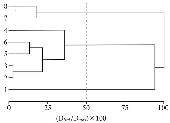
Figure 3.
Dendrogram showing grouping of the sample sites using hierarchical cluster analysis (CA) based on the water quality of the Burío river.
PCA was used to identify the main parameters that spatially affect water quality. Before performing the PCA, suitability of the data was tested using the Kaiser-Meyer-Olkin (>0.5) and Barlett’s sphericity tests (p < 0.05) and was considered satisfactory for PCA [11]. The results are presented in Table 4. The number of principal factors selected were those with Eingenvalues greater than 1 [49], which explain a total variance of 84% of the surface water data. PC1 exhibits 47% of the total variance, with positive loadings on DO and nitrate; and negative loadings on BOD and TP. PC1 can be interpreted to mostly represent runoff and the influence of discharges with a high concentration of organic matter from anthropogenic activities and its degradation processes through the sub-catchment; nitrate can also derive from agriculture zones at the top of the catchment. In PC2, 37% of the total variance is explained with positive loadings on TS, pH, and temperature, which would correspond to landscape variations in LU, natural weathering of the catchment, and wastewater discharges from urban activities.
Table 4.
Principal component analysis (PCA) results in the Burío river.
The spatial trend of the parameters of PC1 are illustrated in Figure 4. DO concentration decrease in the middle of the sub-catchment, where BOD and TP concentration increase; this trend corresponds to the previous cluster group 2. In this section of the river (between sample points 2 and 6), the oxidation of organic matter by microbial activity can be determined by the DO concentration [48], where the lowest value in the dry season at site 4 was 22.8%. After this section, the river channel is wider and the water column narrow, favouring the water oxygenation, oxidant processes, and the level of self-purification of the river. Lower levels of pollution were found at sample point 5, resulting in decreased BOD and TP concentrations—most likely as a result of the increased dilution effect caused by the Quebrada Seca tributary. At sampling point 1, nitrate concentration was high—most likely as a result of the fertilizers applied to the adjacent coffee plantations that according to Cannavo et al. [50] can be estimated up to 50 kg ha−1 yr−1 N.
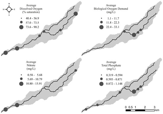
Figure 4.
Spatial variation of dissolved oxygen, biochemical oxygen demand, nitrate, and total phosphate in the Burío river.
Overall, it is challenging to assess and compare water quality parameters within a catchment. The use of WQI simplifies the assessment process and provides useful information for communicating results with policymakers and watershed managers. The seasonal analysis of the NSF-WQI showed that there was a statistically significant difference (F(1, 7) = 7.70, p = 0.008) between the wet season (average = 62.92, SE = 0.92) and the dry season (average = 57.79, SE = 1.57). Nonetheless, regardless of the season, the water quality of the river was classified as “medium”. The spatio-temporal variation is illustrated in Figure 5. The headwaters presented the best condition “good” with values above 71 in both seasons, whilst sample site 4 was classified as “bad” in the dry season. As previously mentioned, site 4 presented the most critical condition in water quality, so special attention must be given by the regulatory authorities. The overall temporal analysis of the NSF-WQI showed that the rivers’ condition remained “medium” during the period of study, even though the concentration of individual parameters (e.g., DO) decreased. Although the results of the water quality index were not sensitive enough to represent the improved water quality before the river mouth, it does provide an important tool for policymakers and watershed managers for assessing regulatory standards, understanding the main causes of pollution, and providing a first step towards remediation strategies.
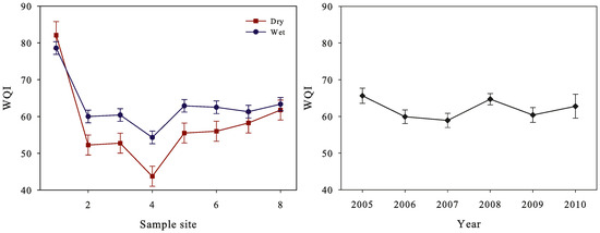
Figure 5.
National Sanitation Foundation water quality index (NSF-WQI) in the Burío river: (left) spatial and seasonal variation and (right) temporal variation.
4. Conclusions
This study has provided valuable information that identified temporal and spatial trends related to surface water quality within a tropical urban sub-catchment. Variations in water quality parameters and the results of the NSF-WQI provided evidence highlighting the vulnerability of the Burío river to pollution from semi-rural, urban, and industrial zones. The industrial activities and urban development in the middle and lower part of the sub-catchment have stimulated the pollution of the river and have decreased the riparian forest, reducing the vegetation damping effect of anthropogenic activities. However, some characteristics of the river such as relief, alterations of the river bed, width, and depth are factors that could be favouring the water oxygenation in the Burío river, attenuating the effects of the human activities. Further studies must be conducted which include a wider range of parameters due to the high amount of wastewater discharges without treatment in the country. In addition, a more sensitive water quality index is also necessary to spatially analyse water quality in small catchments, differentiating LU and pollution sources.
The results of this spatial and temporal surface water quality assessment provide valuable information that allow local governments to formulate evidence-based water resource management strategies. Furthermore, the methodological approach used in this study provides a transitional framework for reducing the number of sample sites, the number of parameters, as well as the number of sample campaigns within a year for similar surface water quality monitoring networks, making them more cost-effective in the long-term for municipalities and decision-makers. This is of particular importance in developing countries where resources are often more limited. Overall, monitoring network results must be used to control pollution—particularly in catchments where urban and industrial activities are rapidly increasing, but also to promote evidence-based environmental policies.
Acknowledgments
This project was financially supported by the Research Office of Universidad Nacional of Costa Rica through grant NX-053545, the Municipalidad de Heredia through the Integral Development Association of San Jorge and the Ministry of Science, Technology and Telecommunications (MICITT) of Costa Rica. The authors thank D. Rojas-Cantillano, J. Herrera-Núnez, F. Arias-González, A. Méndez-Yesca, S. Carvajal-Aguilar, D. Carrillo-López, F. Víquez-Chaves and E. Corrales-Brenes for their collaboration in sample campaigns and laboratory and data analyses.
Author Contributions
Viviana Salgado-Silva, Juana M. Coto-Campos and Cristina Benavides-Benavides conceived, designed and performed the experiments; Leonardo Mena-Rivera made the data analysis; Thomas H. A. Swinscoe made the maps; and Leonardo Mena-Rivera and Thomas H. A. Swinscoe wrote the paper. All the authors contributed to the manuscript.
Conflicts of Interest
The authors declare no conflict of interest.
References
- Sun, W.; Xia, C.; Xu, M.; Guo, J.; Sun, G. Application of modified water quality indices as indicators to assess the spatial and temporal trends of water quality in the Dongjiang River. Ecol. Indic. 2016, 66, 306–312. [Google Scholar] [CrossRef]
- Boeder, M.; Chang, H. Multi-scale analysis of oxygen demand trends in an urbanizing Oregon watershed, USA. J. Environ. Manag. 2008, 87, 567–581. [Google Scholar] [CrossRef] [PubMed]
- Duh, J.D.; Shandas, V.; Chang, H.; George, L.A. Rates of urbanisation and the resiliency of air and water quality. Sci. Total Environ. 2008, 400, 238–256. [Google Scholar] [CrossRef] [PubMed]
- Suthar, S.; Sharma, J.; Chabukdhara, M.; Nema, A.K. Water quality assessment of river Hindon at Ghaziabad, India: Impact of industrial and urban wastewater. Environ. Monit. Assess. 2010, 165, 103–112. [Google Scholar] [CrossRef] [PubMed]
- United Nations World Water Assessment Programm (WWAP). The United Nations World Water Development Report 2016; Technical Report; UNESCO: Paris, France, 2016. [Google Scholar]
- Zeilhofer, P.; Lima, E.B.N.R.; Lima, G.A.R. Spatial patterns of water quality in the Cuiabá River Basin, Central Brazil. Environ. Monit. Assess. 2006, 123, 41–62. [Google Scholar] [CrossRef] [PubMed]
- Singh, K.P.; Malik, A.; Mohan, D.; Sinha, S. Multivariate statistical techniques for the evaluation of spatial and temporal variations in water quality of Gomti River (India)—A case study. Water Res. 2004, 38, 3980–3992. [Google Scholar] [CrossRef] [PubMed]
- Duan, W.; He, B.; Nover, D.; Yang, G.; Chen, W.; Meng, H.; Zou, S.; Liu, C. Water Quality Assessment and Pollution Source Identification of the Eastern Poyang Lake Basin Using Multivariate Statistical Methods. Sustainability 2016, 8, 133. [Google Scholar] [CrossRef]
- Behmel, S.; Damour, M.; Ludwig, R.; Rodriguez, M.J. Water quality monitoring strategies—A review and future perspectives. Sci. Total Environ. 2016, 571, 1312–1329. [Google Scholar] [CrossRef] [PubMed]
- Nnane, D.E.; Ebdon, J.E.; Taylor, H.D. Integrated analysis of water quality parameters for cost-effective faecal pollution management in river catchments. Water Res. 2011, 45, 2235–2246. [Google Scholar] [CrossRef] [PubMed]
- Kim, M.; Kim, Y.; Kim, H.; Piao, W.; Kim, C. Enhanced monitoring of water quality variation in Nakdong River downstream using multivariate statistical techniques. Desalination Water Treat. 2016, 57, 12508–12517. [Google Scholar] [CrossRef]
- Warner, N.R.; Christie, C.A.; Jackson, R.B.; Vengosh, A. Impacts of shale gas wastewater disposal on water quality in western Pennsylvania. Environ. Sci. Technol. 2013, 47, 11849–11857. [Google Scholar] [CrossRef] [PubMed]
- Wunderlin, D.A.; Díaz, M.d.P.; Amé, M.V.; Pesce, S.F.; Hued, A.C.; Bistoni, M.d.l.Á. Pattern Recognition Techniques for the Evaluation of Spatial and Temporal Variations in Water Quality. A Case Study: Suquía River Basin (Córdoba, Argentina). Water Res. 2001, 35, 2881–2894. [Google Scholar]
- Duan, W.; He, B.; Takara, K.; Luo, P.; Nover, D.; Sahu, N.; Yamashiki, Y. Spatiotemporal evaluation of water quality incidents in Japan between 1996 and 2007. Chemosphere 2013, 93, 946–953. [Google Scholar] [CrossRef] [PubMed]
- Duan, W.; Takara, K.; He, B.; Luo, P.; Nover, D.; Yamashiki, Y. Spatial and temporal trends in estimates of nutrient and suspended sediment loads in the Ishikari River, Japan, 1985 to 2010. Sci. Total Environ. 2013, 461–462, 499–508. [Google Scholar] [CrossRef] [PubMed]
- Wallace, J.; Stewart, L.; Hawdon, A.; Keen, R.; Karim, F.; Kemei, J. Flood water quality and marine sediment and nutrient loads from the Tully and Murray catchments in north Queensland, Australia. Mar. Freshw. Res. 2009, 60, 1123. [Google Scholar] [CrossRef]
- Ongley, E.D. Water Quality Programs in Developing Countries. Water Int. 2001, 26, 14–23. [Google Scholar] [CrossRef]
- Giri, S.; Qiu, Z. Understanding the relationship of land uses and water quality in Twenty First Century: A review. J. Environ. Manag. 2016, 173, 41–48. [Google Scholar] [CrossRef] [PubMed]
- Levine, C.R.; Yanai, R.D.; Lampman, G.G.; Burns, D.A.; Driscoll, C.T.; Lawrence, G.B.; Lynch, J.A.; Schoch, N. Evaluating the efficiency of environmental monitoring programs. Ecol. Indic. 2014, 39, 94–101. [Google Scholar] [CrossRef]
- Laino-Guanes, R.; González-Espinosa, M.; Ramírez-Marcial, N.; Bello-Mendoza, R.; Jiménez, F.; Casanoves, F.; Musálem-Castillejos, K. Human pressure on water quality and water yield in the upper Grijalva river basin in the Mexico-Guatemala border. Ecohydrol. Hydrobiol. 2016, 16, 149–159. [Google Scholar] [CrossRef]
- Jung, K.Y.; Lee, K.L.; Im, T.H.; Lee, I.J.; Kim, S.; Han, K.Y.; Ahn, J.M. Evaluation of water quality for the Nakdong River watershed using multivariate analysis. Environ. Technol. Innov. 2016, 5, 67–82. [Google Scholar] [CrossRef]
- Wang, Y.B.; Liu, C.W.; Liao, P.Y.; Lee, J.J. Spatial pattern assessment of river water quality: Implications of reducing the number of monitoring stations and chemical parameters. Environ. Monit. Assess. 2014, 186, 1781–1792. [Google Scholar] [CrossRef] [PubMed]
- Ouyang, Y.; Nkedi-Kizza, P.; Wu, Q.T.; Shinde, D.; Huang, C.H. Assessment of seasonal variations in surface water quality. Water Res. 2006, 40, 3800–3810. [Google Scholar] [CrossRef] [PubMed]
- Hoseinzadeh, E.; Khorsandi, H.; Wei, C.; Alipour, M. Evaluation of Aydughmush River water quality using the National Sanitation Foundation Water Quality Index (NSFWQI), River Pollution Index (RPI), and Forestry Water Quality Index (FWQI). Desalination Water Treat. 2015, 54, 2994–3002. [Google Scholar] [CrossRef]
- Onestini, M. Water Quality and Health in Poor Urban Areas of Latin America. Int. J. Water Res. Dev. 2011, 27, 219–226. [Google Scholar] [CrossRef]
- Groppo, J.D.; De Moraes, J.M.; Beduschi, C.E.; Genovez, A.M.; Martinelli, L.A. Trend analysis of water quality in some rivers with different degrees of development within the São Paulo State, Brazil. River Res. Appl. 2008, 24, 1056–1067. [Google Scholar] [CrossRef]
- World Health Organisation (WHO). Global Water Supply and Sanitation 2000 Report; Technical Report; World Health Organisation: Geneva, Switzerland, 2000. [Google Scholar]
- Bower, K.M. Water supply and sanitation of Costa Rica. Environ. Earth Sci. 2014, 71, 107–123. [Google Scholar] [CrossRef]
- Reynolds-Vargas, J.; Fraile-Merino, J.; Hirata, R. Trends in Nitrate Concentrations and Determination of its Origin Using Stable Isotopes (18O and 15N) in Groundwater of the Western Central Valley, Costa Rica. AMBIO 2006, 35, 229–236. [Google Scholar] [CrossRef] [PubMed]
- Instituto Meteorológico Nacional de Costa Rica. Available online: http://www.imn.ac.cr (accessed on 1 February 2017).
- Ministerio de Salud de Costa Rica. Available online: http://www.ministeriodesalud.go.cr (accessed on 15 February 2017).
- APHA; AWWA; WEF. Standard Methods for the Examination of Water & Wastewater; Standard Methods for the Examination ofWater and Wastewater; American Public Health Association: Washington, DC, USA, 2005. [Google Scholar]
- Farnham, I.M.; Singh, A.K.; Stetzenbach, K.J.; Johannesson, K.H. Treatment of nondetects in multivariate analysis of groundwater geochemistry data. Chemom. Intell. Lab. Syst. 2002, 60, 265–281. [Google Scholar] [CrossRef]
- Araujo, H.A.; Cooper, A.B.; Hassan, M.A.; Venditti, J. Estimating suspended sediment concentrations in areas with limited hydrological data using a mixed-effects model. Hydrol. Process. 2012, 26, 3678–3688. [Google Scholar] [CrossRef]
- Ward, J.H. Hierarchical Grouping to Optimize an Objective Function. J. Am. Stat. Assoc. 1963, 58, 236–244. [Google Scholar] [CrossRef]
- Ouyang, Y. Evaluation of river water quality monitoring stations by principal component analysis. Water Res. 2005, 39, 2621–2635. [Google Scholar] [CrossRef] [PubMed]
- Olsen, R.L.; Chappell, R.W.; Loftis, J.C. Water quality sample collection, data treatment and results presentation for principal components analysis—Literature review and Illinois River watershed case study. Water Res. 2012, 46, 3110–3122. [Google Scholar] [CrossRef] [PubMed]
- Di Rienzo, J.; Casanoves, F.; Balzarini, M.; Gonzalez, L.; Tablada, M.; Robledo, C. Infostat—Sofware Estadístico; Universidad Nacional de Córdoba: Córdoba, Argentina, 2015. [Google Scholar]
- R Core Team. R: A Language and Environment for Statistical Computing; R Foundation for Statistical Computing: Vienna, Austria, 2016. [Google Scholar]
- Brown, R.M.; McClelland, N.I.; Deininger, R.A.; Tozer, R.G. A water quality index- Do we dare? Water Sew. Works 1970, 117, 339–343. [Google Scholar]
- U.S. Environmental Protection Agency. Quality Criteria for Water; United States Environmental Protection Agency: Washington, DC, USA, 1986; p. 447. [Google Scholar]
- Uriarte, M.; Yackulic, C.B.; Lim, Y.; Arce-Nazario, J.A. Influence of land use on water quality in a tropical landscape: A multi-scale analysis. Landsc. Ecol. 2011, 26, 1151–1164. [Google Scholar] [CrossRef] [PubMed]
- Calvo Brenes, G.; Mora Molina, J. Contaminación fecal en varios ríos de la Gran Área Metropolitana y la Península de Osa. Tecnol. Marcha 2012, 25, 33–39. [Google Scholar] [CrossRef]
- MINAE. Reglamento para la evaluación y clasificación de la calidad de cuerpos de agua superficiales. Decreto, No. 33903. La Gaceta 2007, 178, 1–21. [Google Scholar]
- Calvo, G.; Mora, J. Evaluación y clasificación preliminar de la calidad del agua de la cuenca del río Tárcoles y el Reventazón. Tecnol. Marcha 2007, 20, 7. [Google Scholar]
- Herrera, J.; Rodríguez, S.; Rojas, J.F.; Herrera, É.; Chaves, M. Variación temporal y espacial de la calidad de las aguas superficiales en la subcuenca del río Virilla (Costa Rica) entre 2006 y 2010. Rev. Cienc. Ambient. 2013, 45, 51–62. [Google Scholar] [CrossRef]
- Mukaka, M.M. Statistics corner: A guide to appropriate use of correlation coefficient in medical research. Malawi Med. J. 2012, 24, 69–71. [Google Scholar] [PubMed]
- Chapman, D. Water Quality Assessments—A Guide to Use of Biota, Sediments and Water in Enviromental Monitoring; Cambridge University Press: Cambridge, UK, 1996; Volume 1, p. 609. [Google Scholar]
- Yeomans, K.A.; Golder, P.A. The Guttman-Kaiser Criterion as a Predictor of the Number of Common Factors. J. R. Stat. Soc. Ser. D: Stat. 1982, 31, 221–229. [Google Scholar] [CrossRef]
- Cannavo, P.; Harmand, J.M.; Zeller, B.; Vaast, P.; Ramírez, J.E.; Dambrine, E. Low nitrogen use efficiency and high nitrate leaching in a highly fertilized Coffea arabica-Inga densiflora agroforestry system: A 15N labeled fertilizer study. Nutr. Cycl. Agroecosyst. 2013, 95, 377–394. [Google Scholar] [CrossRef]
© 2017 by the authors. Licensee MDPI, Basel, Switzerland. This article is an open access article distributed under the terms and conditions of the Creative Commons Attribution (CC BY) license (http://creativecommons.org/licenses/by/4.0/).