Improved Medium- and Long-Term Runoff Forecasting Using a Multimodel Approach in the Yellow River Headwaters Region Based on Large-Scale and Local-Scale Climate Information

Abstract

Medium- and long-term runoff forecasting is essential for hydropower generation and water resources coordinated regulation in the Yellow River headwaters region. Climate change has a great impact on runoff within basins, and incorporating different climate information into runoff forecasting can assist in creating longer lead-times in planning periods. In this paper, a multimodel approach was developed to further improve the accuracy and reliability of runoff forecasting fully considering of large-scale and local-scale climatic factors. First, with four large-scale atmospheric oscillations, sea surface temperature, precipitation, and temperature as the predictors, multiple linear regression (MLR), radial basis function neural network (RBFNN), and support vector regression (SVR) models were built. Next, a Bayesian model averaging (BMA)-based multimodel was developed using weighted MLR, RBFNN, and SVR models, and the performance of the BMA-based multimodel was compared to those of the MLR, RBFNN, and SVR models. Finally, the high-runoff performance of these four models was further analyzed to prove the effectiveness of each model. The BMA-based multimodel performed better than those of the other models, as well as high-runoff forecasting. The results also revealed that the performance of the forecasting models with multiple climatic factors were generally superior to that without climatic factors. The BMA-based multimodel with climatic factors not only provides a promising, reliable method for medium- and long-term runoff forecasting, but also facilitates uncertainty estimation under different confidence intervals.

1. Introduction

The headwaters of China’s Yellow River comprise an important source of freshwater resources, contributing nearly 40% of the total amount available in the Yellow River basin [1,2]. Reliable and accurate medium- and long-term runoff forecasting plays an important role in hydropower generation and in the coordinated regulation of water resources so that decision-makers know the quantity of water available in the basin over long periods of time, and can facilitate efficient management of water resources for a multitude of competitive applications in the region [3,4]. According to different forecast periods, runoff forecasting can be divided into short-term forecasting (e.g., hourly or daily), medium- and long-term forecasting (e.g., weekly, monthly, and seasonal), and long-term forecasting (e.g., annual), so medium- and long-term forecasting refers to runoff forecasting at the monthly scale in this paper. The Yellow River headwaters region is located in the northeast of the Tibetan Plateau, which is very sensitive to climate change and rarely influenced by human activities. Climate change has a great impact on runoff within basins, especially in climate-sensitive areas [5]. There is a complex non-linear relationship between different climatic factors and runoff, and it is difficult to understand such complex relationships and build an accurate runoff forecasting model at medium- and long-term time scales [6,7].

Multiple climatic factors as the input variables are different for runoff forecasting in different regions. Abudu et al. [8] used a stochastic hybrid modeling approach for forecasting monthly streamflow in the Rio Grande headwaters basin, and the input variables were antecedent runoff, precipitation and snow water equivalent. Evsukoff et al. [9] presented the development of a recurrent fuzzy system model for the Iguaçu River basin in southern Brazil, and the input variable was only rainfall. Talei et al. [10] applied a Takagi-Sugeno neuro-fuzzy model with online learning for runoff forecasting for three different catchments, and the input variable was the antecedent rainfall. Elsanabary and Gan [11] developed artificial neural networks with a genetic algorithm for forecasting weekly streamflow of the Upper Blue Nile basin, and the input variables were monthly precipitation and sea surface temperature. Djibo et al. [12] used a probabilistic approach statistical seasonal streamflow forecasting over West African Sahel; the input variables were sea level pressure, relative humidity, and air temperature. Biondi and De Luca [13,14] considered a simple lumped and conceptual rainfall-runoff model for design flood estimation in gauged and ungauged catchments in southern Italy, by considering as input 500-years of 20-min synthetic rainfall data, derived from a daily rainfall generator and a specific downscaling procedure for Southern Italy. Previous studies primarily focused on precipitation and antecedent runoff as the inputs for runoff forecasting, however, less attention was paid to fully incorporate large-scale climate variables and other local-scale climate variables as the inputs.

Runoff forecasting has always been a tremendous challenge for water resource management engineers and decision-makers, and a wide variety of models have been applied to runoff forecasting. Runoff forecasting approaches can be divided into two categories: one is based on physical processes, which require an accurate description of runoff processes and, thus, its applicability is limited by large variations in space and time. The other is the data-driven approach, which attempts to use historical climate factors and runoff data features to forecast runoff in the future. Although data-driven approaches may lack the ability to provide physical interpretation, they are becoming increasingly popular for providing relatively the accurate flow forecasts with their rapid development and less information requirements than hydrological models need. Different data-driven models have the ability to capture the randomicity, periodicity, and volatility of runoff processes, and multimodel techniques can obtain accurate and comprehensive information on different characteristic and improve forecasting accuracy by linearly combining two or more models according to different weighting strategies. A number of multimodel methods have been developed for runoff forecasting. Block et al. [15] presented the coupling of global climate models (GCMs), multiple regional climate models, and numerous water balance models to improve stream flow forecasting compared to any individual model. Zhang et al. [16] proposed singular spectrum analysis and the autoregressive integrated moving average (ARIMA) hybrid model for annual runoff forecasting. It was shown that the hybrid model exhibited the best predictive performance compared to ARIMA and singular spectrum analysis-linear recurrent formulae (SSA-LRF) models. Wang et al. [17] presented an artificial neural network (ANN) model coupled with ensemble empirical mode decomposition (EEMD) for forecasting medium- and long-term runoff time series, and the proposed EEMD-ANN model attained a significant improvement over the ANN approach alone in medium- and long-term runoff time series forecasting. Recently, the Bayesian model averaging (BMA)-based multimodel has gained popularity as a multimodel because it can provide a more realistic forecast that considers both between-model variances and in-model variances.

As the main water source for Yellow River, the variations in Yellow River headwater runoff greatly affect downstream discharge and available water supply and, therefore, it has attracted more and more attention from researchers. Zheng et al. [18] have investigated changes in the stream flow regime in the headwater catchments of the Yellow River basin since the 1950s. The results showed no significant trend for the period 1956–2000, but reported that a significant change in annual stream flow occurred around 1990. Lan et al. [19] analyzed the response of the runoff in the headwater region to climate change and reasonableness of the response based on the data measured during the period 1959–2008. Recently, sporadic explorations have been conducted of medium- and long-term runoff forecasting in the Yellow River headwaters region. Wang et al. [20] developed three forms of hybrid artificial neural networks (ANNs) to forecast stream flows for the upper Yellow River. Zhang et al. [21] combined wavelet analysis (WA) and an ANN for runoff time series prediction in the headwaters area. However, few studies have adopted the BMA-based multimodel forecasting model for runoff forecasting, especially with a number of large-scale climatic indices, so it is an attempt to improve the accuracy of runoff forecasting in Yellow River headwaters region.

In this paper, the monthly runoff data from Tangnaihai station in the Yellow River headwaters region was analyzed as the case study. Four atmospheric oscillations, sea surface temperature in different areas, precipitation and temperature were fully considered as the inputs for runoff forecasting. First, multiple linear regression (MLR), radial basis function neural network (RBFNN), and support vector regression (SVR) models were built based on multiple climatic factors, and an investigation of how the main parameters influenced the performance of the SVR model was undertaken, and the best parameters were selected for medium- and long-term runoff forecasting. Then a BMA-based multimodel was developed using weighted models (MLR, RBFNN, and SVR) to further improve medium- and long-term runoff forecasting, and provide uncertainty estimation under different confidence intervals. The performance of the four models for high runoff was further analyzed to prove the effectiveness of each model. Finally, the multimodel, with and without climatic factors, were also built for comparison.

2. Materials and Methods

In this paper, the data-driven models, including multiple linear regression, radial basis function neural network, support vector regression, and a Bayesian model averaging-based multimodel were developed, and data-driven models are actually black box models, which extract the input-output relationship from the historical record of climate data and runoff to provide simplified representations of the complex nonstationary hydrological systems. Thus, the length and quality of the observed climate factors and runoff time series will determine the accuracy of the model, but once the length and quality of the observed runoff series are fixed, the parameters of models are dominant on the accuracy of the model.

2.1. Multiple Linear Regression

The multiple linear regression (MLR) model as a popular statistical time series model, is often used to predict values in the future; and it is built as follows:

$$y={\beta }_1{x}_1+{\beta }_2{x}_2+\dots +{\beta }_k{x}_k+{\beta }_0$$

(1)

where k is the number of the predictors, ${\beta }_i$ are regression coefficients calculated by the least-squares method, and $x$ is the climatic factor [22].

2.2. Radial Basis Function Neural Network

The radial basis function neural network (RBFNN) is a typical feed-forward neural network often used for strict interpolation in multidimensional space. The RBFNN consists of one input layer, one hidden layer with a nonlinear RBF activation function, and one output layer with entirely different roles [23,24,25].

From the input layer to the hidden layer, a Gaussian transfer function is used for the hidden neurons, so the transformation is nonlinear; it can be expressed as follows:

$${\phi }_i(x)=\exp \left(-\frac{{\Vert x-x_i\Vert }^2}{2{\sigma }_i{}^2}\right)i=1,2,\dots ,N$$

(2)

where ${\phi }_i\left(x\right)$ is the center of the basis function, ${\sigma }_i$ is the spread of the radial basis function in the ith hidden node, N is the number of hidden nodes, and $\Vert x-x_i\Vert$ is the radial distance between x and the RBF function center. The nonlinear nodes of the hidden layer are centered so that each of them is specialized on a particular zone of the input space [26,27].

However, the transformation from the hidden layer to the output layer is linear, and it is denoted as the weighted summation of the outputs of all hidden nodes connected to the output nodes:

$$f(x)={\displaystyle \sum _{i=1}^N{\omega }_i{\phi }_i\left(x\right)}$$

(3)

where ${\omega }_i$ are the weights of the linear output nodes [28]. The aim of an RBF network is to determine centers, widths, and the linear output weights linking the RBFs to the output nodes layer.

2.3. Support Vector Regression

Support vector regression (SVR), developed from support vector machines (SVMs), is a promising technique for dealing with forecasting problems based on Vapnik-Chervonenkis dimension theory and the structure risk minimization principle. Compared to conventional artificial neural networks, it has better generalization ability with structural risk minimization instead of training error minimization [29,30].

The linear regression estimating function can be written as follows:

$$f\left(x\right)=\omega \varphi \left(x\right)+b$$

(4)

where $\varphi \left(x\right)$ is a nonlinear mapping from the input space to a high-dimensional feature space, b is a threshold value, and $\omega$ is a weight vector, which can be estimated by minimizing the following regularized risk function:

$$R\left(C\right)=\left(C{\displaystyle \sum _{\mathrm{i}=1}^{\mathrm{N}}{\mathrm{L}}_{\epsilon }\left(d_i,y_i\right)}\right)+\frac{1}{2}{\Vert \omega \Vert }^2$$

(5)

The function ${\mathrm{L}}_{\epsilon }\left(d,y\right)$, called the $\epsilon$-insensitive loss function, is given by the formula:

$${\mathrm{L}}_{\epsilon }\left(d,y\right)=\{\begin{array}{c}0\left|d-y\right|\le \epsilon \\ \left|d-y\right|-\epsilon \left|d-y\right|>\epsilon \end{array}$$

(6)

C determines the tradeoff between flatness and the empirical risk; $\epsilon$ is considered to measure empirical error with Vapnik’s linear loss function.

Two slack variables $\xi$ and ${\xi }^{\prime }$ can be incorporated into the regularized risk function to yield the following formulation:

$$R\left(\omega ,\xi ,{\xi }^{\prime },\epsilon \right)=\frac{1}{2}{\Vert \omega \Vert }^2+\mathrm{C}{\displaystyle \sum _{i=1}^N\left(\xi +{\xi }^{\prime }\right)}$$

(7)

subject to:

$$\{\begin{array}{c}\left({\omega }^T\varphi \left(x_i\right)+b\right)-y_i\le \epsilon +\xi \\ y_i-\left({\omega }^T\varphi \left(x_i\right)+b\right)\le \epsilon +{\xi }^{\prime }\\ \xi ,{\xi }^{\prime }\ge 0\end{array}$$

(8)

This constrained optimization problem can be written as a Lagrangian function:

$$\nu \left({\alpha }_i,{\alpha }_i^{*}\right)=-\frac{1}{2}{\displaystyle \sum _{i=1}^N{\displaystyle \sum _{j=1}^N\left({\alpha }_i-{\alpha }_i^{*}\right)({\alpha }_j-{\alpha }_j^{*})}}k\left(x_i,x_j\right)+{\displaystyle \sum _{i=1}^N\left({\alpha }_i-{\alpha }_i^{*}\right)d_i}$$

(9)

subject to:

$$\begin{array}{l}{\displaystyle \sum _{i=1}^N\left({\alpha }_i-{\alpha }_i^{*}\right)=0}{\displaystyle \sum _{i=1}^N\left({\alpha }_i-{\alpha }_i^{*}\right)\le C}\\ {\alpha }_i\ge 0{\alpha }_i^{*}\ge 0i=1,2,\dots ,N\end{array}$$

(10)

and an optimal weight vector of the regression model is:

$$\omega ={\displaystyle \sum _{i=1}^N\left({\alpha }_i-{\alpha }_i^{*}\right)}\varphi \left(x\right)$$

(11)

and so the linear regression in. Equation (11) becomes:

$$f\left(x\right)={\displaystyle \sum _{i=1}^N\left({\alpha }_i-{\alpha }_i^{*}\right)}k\left(x_i,x\right)+b$$

(12)

where $k\left(x_i,x_j\right)$ denotes the inner product of two vectors in the feature space $\varphi \left(x_i\right)$ and $\varphi \left(x_j\right)$, and the Gaussian kernel function is the most commonly used kernel function.

When the length and quality of the training samples are fixed, three parameters are dominated the accuracy of the SVR model: C, which controls the empirical risk degree of the SVR, $\epsilon$, which controls the width of the tube in the loss function; and $\sigma$, which controls the Gaussian function width of the kernel function [31,32,33].

2.4. Bayesian Model Averaging-Based Multimodel

The Bayesian model averaging (BMA)-based multimodel is the average of the considered models weighted by the likelihood that a considered model is correct given the observations, it has been used in various fields, such as statistics, geology, and hydrologic applications. The BMA model provides a more reliable description of the total predictive uncertainty, including the between-model-variance and the within-model-variance, than the original multimodels [34,35].

Consider that $f=\left[f_1,f_2,\cdots ,f_K\right]$ is an ensemble of K considered models and $M=\left[y_1,y_2,\cdots ,y_T\right]$ are observational datasets with data length T, the BMA predictive probability density functions (PDFs) are then:

$$p(y|M)={\displaystyle \sum _{k=1}^{K}p\left(f_k|M\right)}\ast p_k\left(y|f_k,M\right)$$

(13)

where $p\left(f_k|M\right)$ is the posterior probability of model prediction $f_k$; that is, the likelihood of the model prediction being correct given the observational data M. If we denote $w_k=p\left(f_k|M\right)$, we should obtain ${\displaystyle \sum _{k=1}^K{w}_k}=1$. The posterior mean and variance of the BMA prediction can be expressed as:

$$E(\mathrm{y}|M)={{\displaystyle \sum _{k=1}^{K}p\left(f_k|M\right)w_k\left(f_k-{\displaystyle \sum _{i=1}^K{w}_i{f}_i}\right)}}^2+{\displaystyle \sum _{k=1}^K{w}_k{\sigma }_k^2}$$

(14)

$$\mathrm{var}(\mathrm{y}|M)={{\displaystyle \sum _{k=1}^K{w}_k\left(f_k-{\displaystyle \sum _{i=1}^K{w}_i{f}_i}\right)}}^2+{\displaystyle \sum _{k=1}^K{w}_k{\sigma }_k^2}$$

(15)

where ${\sigma }_k^2$ is the variance associated with model prediction.

An expectation-maximization (EM) algorithm was used to estimate $w_k$ and ${\sigma }_k^2$. If $\theta =\left(w_k,{\sigma }_k^2,\cdots ,k=1,2,\cdots ,K\right)$, the log-likelihood function can be approximated as:

$$l\left(\theta \right)=\log \left({\displaystyle \sum _{k=1}^K{w}_k}\ast p_k\left(y|f_k,M\right)\right)$$

(16)

For this study, a latent variable $z_{k,t}$ is introduced:

$$z_{k,t}=\{\begin{array}{c}1\\ 0\end{array}\begin{array}{c}\mathrm{the}k\mathrm{th}\mathrm{model}\mathrm{ensemble}\mathrm{is}\mathrm{the}\mathrm{best}\mathrm{prediction}\mathrm{at}\mathrm{time}t\\ \mathrm{otherwise}\end{array}$$

(17)

At any time t, there is only one $z_{k,t}$ equal to 1, and the rest are equal to 0. The EM algorithm starts with an initial value for the parameter $\theta$. In the expectation (E) step, $z_{k,t}$ is estimated given the current guess of $\theta$. In the maximization (M) step, $\theta$ is estimated given the current values of $z_{k,t}$. The EM steps are repeated until certain convergence criteria are satisfied.

2.5. Model Performance Evaluation

Four standard statistical measures, root-mean-square error (RMSE), mean relative error (MAE), Nash-Sutcliffe (NS) efficiency coefficient, and determination coefficient (R²), are employed to evaluate the performance of all the forecasting models.

(1) RMSE:

$$\mathrm{RMSE}=\sqrt{\frac{{\displaystyle \sum _{i=1}^n{\left(q_i-Q_i\right)}^2}}{N}}$$

(18)

where $q_i$ and $Q_i$ are the observed and predicted data at the ith time period, respectively, and N is the number of considered data.

RMSE is frequently used to measure the residual between observed and predicted runoff.

(2) MAE:

$$\mathrm{MAE}=\frac{1}{N}{\displaystyle \sum _{i=1}^n\left|Q_i-q_i\right|}$$

(19)

MAE indicates the mean deviation between observed and predicted runoff.

(3) NS efficiency coefficient:

$$\mathrm{NS}=1-\frac{{\displaystyle \sum _{i=1}^n{\left(q_i-Q_i\right)}^2}}{{\displaystyle \sum _{i=1}^n{\left(q_i-{\overline{q}}_i\right)}^2}}$$

(20)

where ${\overline{q}}_i$ is the mean observed runoff. The NS efficiency coefficient is used to measure the capability of the model to forecast runoff away from the mean, which is sensitive to extreme values.

(4) R²:

$${\mathrm{R}}^2={\left[\frac{{\displaystyle \sum _{i=1}^n\left(q_i-{\overline{q}}_i\right)\left(Q_i-{\overline{Q}}_i\right)}}{\sqrt{{\displaystyle \sum _{i=1}^n{\left(q_i-{\overline{q}}_i\right)}^2{\displaystyle \sum _{i=1}^n{\left(Q_i-{\overline{Q}}_i\right)}^2}}}}\right]}^2$$

(21)

where ${\overline{Q}}_{\mathrm{i}}$ is the mean predicted runoff.

R² evaluates the linear correlation by summarizing the discrepancy between the observed and predicted runoff. The values of NS and R² range between 0 and 1.0. Essentially, the smaller the RMSE and MAE is, the more accurate the runoff expectation is; and the closer NS and R² is to 1, the more accurate the runoff expectation is.

3. Study Area

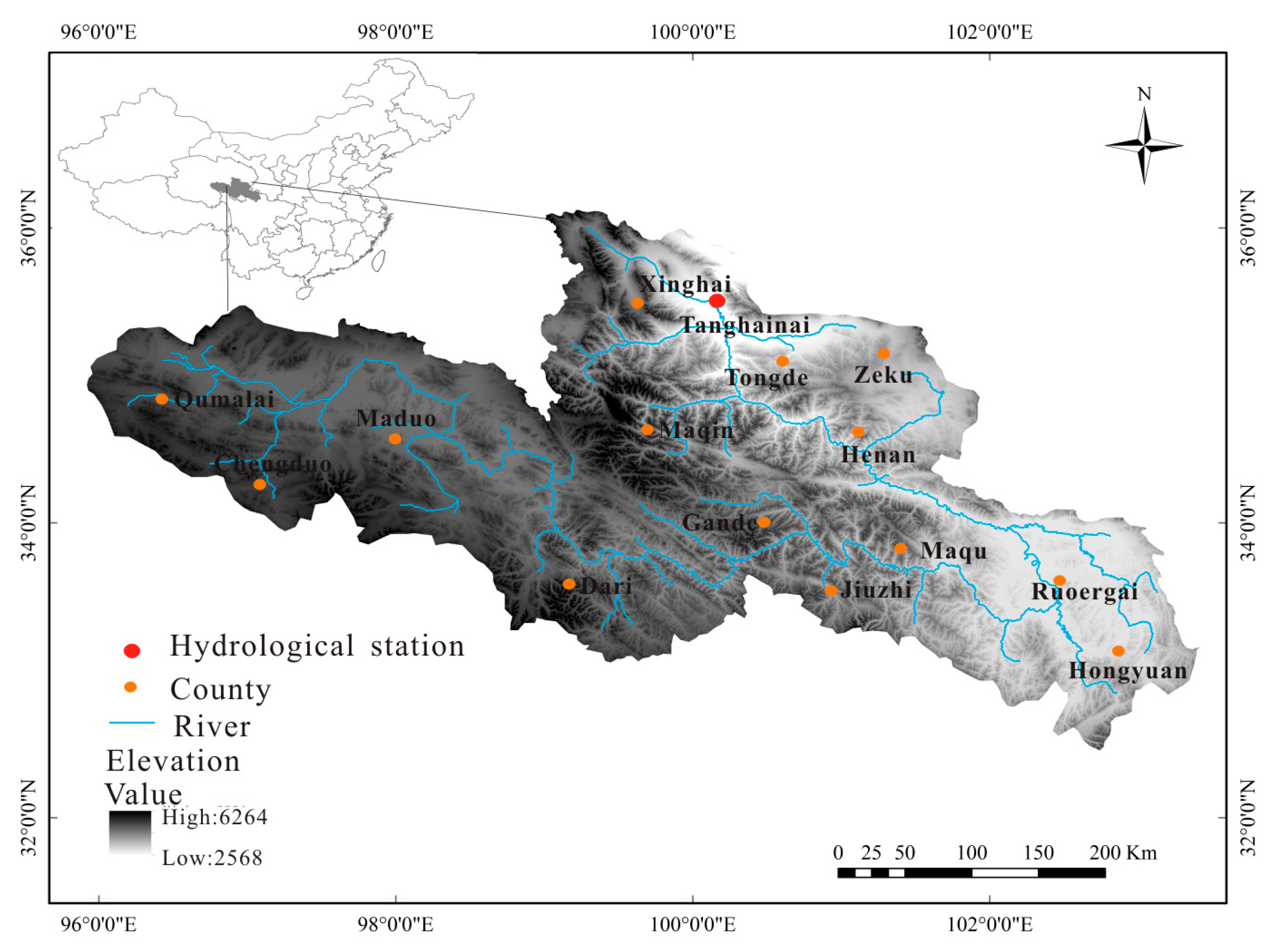
The Tangnaihai hydrological station is the control station for the largest reservoir in the upstream part of the Yellow River, which also serves as the control outlet of the basin; and it is sensitive to climate changes. There are no large hydraulic engineering mechanisms in place, so runoff is only slightly influenced by human activities. Therefore, runoff forecasting has important significance for predicting ecological water demand, flood control operation, water allocation, and hydropower scheduling for the Yellow River.

The study area is located in the eastern part of Qinghai Province between latitudes 32°5′ N–36°30′ N and longitudes 95°30′ E–103°30′ E, including Maduo, Maqin, Jiuzhi, Dari, Hongyuan, Ruoergai, Xinghai, Tongde, Zeku, and Henan counties, among others, and covers an area approximately 12.20 × 10⁴ km² in size above Tangnaihai station (Figure 1). The average elevation is approximately 4217 m and ranges from 2568 to 6264 m. It has a typical plateau continental monsoon region climate; the annual temperature difference is small, but the daily temperature difference is significant. The annual average temperature in the study area ranges from −5.38 °C to 4.14 °C, the annual average evaporation ranges between 730 and 1700 mm, the annual average rainfall ranges between 262.2 and 772.8 mm, and the average annual runoff of the Yellow River at Tangnaihai station is 1.39 × 10¹⁰ m³.

Here, four climatic indices, sea surface temperatures in different areas (SST), precipitation, and temperature were used. The climatic indices included the strength of the East Asian trough (EAT), West Pacific Subtropical High (WPSH), Northern Hemisphere polar vortex (NH), Tibetan Plateau Index B (TPI-B). Monthly EAT, WPSH, NH, and the TPI-B data used were retrieved from the Climate Prediction Center of the US National Oceanic and Atmospheric Administration. Monthly temperature (T) and precipitation (P) from 1956 to 2014 were obtained from the China Meteorological Administration. Sea surface temperature data during 1956–2014 were obtained from Met Office Hadley Centre observation datasets. Three zones of monthly SST were used: zone 1 (90° E–105° E, 30° S–35° S), zone 2 (122.5° E–177.5° E, 17.5° N–27.5° N), and zone 3 (160° E–170° E, 25° S–35° S).

In this study, the monthly runoff data from Tangnaihai station were selected for model calibration and validation. The dataset for the period January 1956–December 2010 was used for model calibration and the dataset for January 2011–December 2014 for model validation.

4. Results and Discussion

4.1. BMA-Based Multi Model Modeling Process

The BMA-based multi model was developed based on the MLR, RBFNN, and SVR models; hence, the SVR model, RBFNN model, and MLR model were first employed for forecasting medium- and long-term runoff. Then, an SVR model was selected as an example to illustrate the modeling process, and a detailed analysis of how the main parameters influenced the performance of the SVR model was performed.

The SVR model was built for monthly runoff forecasting, and the model-calibration process was carried out to obtain the optimal parameters and so that, finally, runoff forecasting could be conducted according to the training parameters. In the application, nine input variables including monthly EAT, WPSH, NH, TPI-B, three zones of monthly SST (SST1, SST2, SST3), evaporation, temperature, and precipitation, and the corresponding monthly runoff were used as the output, details of validation samples are presented in

Table 1. Input-output pairs for model-validation process.

Sample	Input									Output
	WPSH	EAT	NH	TPI-B	SST1	SST2	SST3	P	T	Runoff
1	1	64	271	470	20	17	23	76	−12	179
2	0	113	360	492	21	16	24	8	−7	158
3	3	103	304	516	21	16	24	139	−6	216
4	12	190	220	548	19	17	23	234	1	384
5	36	226	143	574	18	18	22	693	5	460
6	62	226	115	578	17	19	20	1071	8	1170
…	…	…	…	…	…	…	…	…	…	…
42	29	274	116	580	17	18	20	1152	9	969
43	47	274	99	596	16	21	19	591	11	958
44	47	274	125	595	16	22	19	1788	10	1043
45	43	305	195	595	15	22	19	733	7	1454
46	18	236	253	576	16	21	19	223	1	1016
47	37	176	279	543	18	20	21	33	−4	455
48	20	89	301	521	19	18	22	83	−11	273

.

The important part in building a SVR model is training the parameters, including the regularization parameter, spread and tube width, which significantly influence forecasting accuracy. Hence, the parameters should be selected carefully.

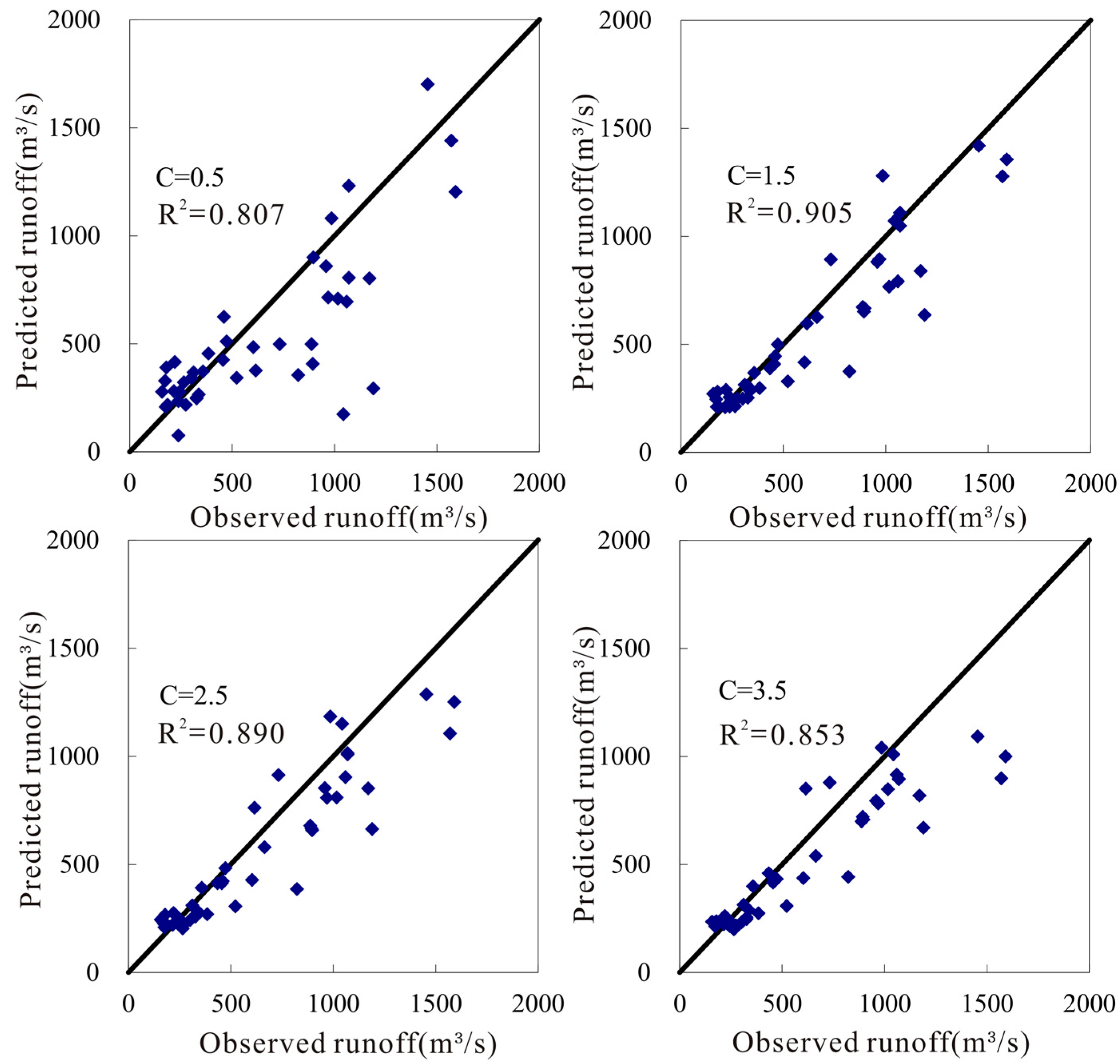
The optimal parameters were determined by trial and error, and are as follows: the spread $\sigma$ ranges from 0.1 to 10, the regularization parameter $C$ from 0.1 to 10, and the tube width $\epsilon$ from 0.0001 to 0.1. The optimal values of the three parameters were selected when R² reached its maximum value as the values of the three parameters changed. Figure 2 shows the changing accuracy of the test datasets when the spread $\sigma =0.6$, the tube width $\epsilon =0.001$ and the regularization parameter $C$ values were 0.5, 1.5, 2.5, and 3.5.

As shown in Figure 2, in the model-validation process, when $C$ = 0.5, R² was approximately 0.807, and when $C$ = 2.5, R² was approximately 0.890, when $C$ = 3.5, R² was approximately 0.853. The results show that the best value for regularization parameter $C$ was 1.5 with R² approximately 0.905. Hence, the SVR model using a regularization parameter $C$ value of 1.5 was selected for monthly runoff forecasting in this study. In addition, regularization parameter $C$ = 1.5, spread $\sigma =0.6$, and regression tube width $\epsilon =0.001$ were selected as the other optimal parameters for runoff forecasting at Tangnaihai station.

RBFNN and MLR models were also applied for forecasting monthly runoff, and based on the MLR, RBFNN, and SVR models, a multimodel approach was developed to further improve the accuracy and reliability of medium- and long-term runoff forecasting. A BMA-based multimodel was developed for more reliable probabilistic runoff forecasting, which inferred consensus predictions by weighing individual predictions. The weights for the three models, MLR, RBF, and SVR were 0.005, 0.140, and 0.875, respectively. The results indicated the better an individual model performed, the higher the weight of that individual model is.

4.2. Comparative Analysis of MLR, RBFNN, SVR, and BMA-Based Multimodels

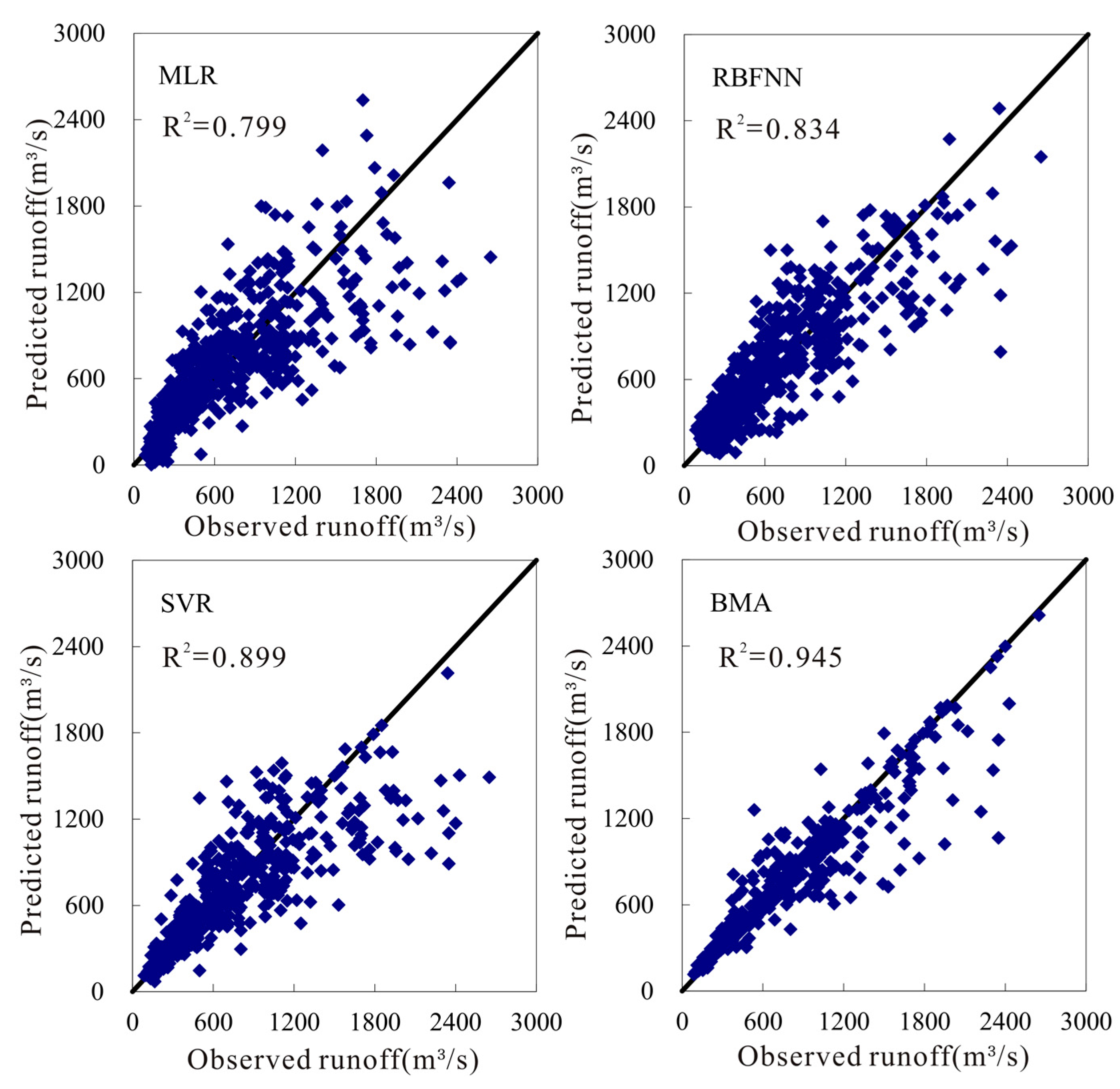
The results from the BMA-based multimodel were compared to those of the MLR, RBFNN, and SVR models, and the results of the comparison are shown in Figure 3. It can be seen that the SVR and RBFNN models performed better than the MLR model during the model-calibration process, and that the MLR model generally underestimated the monthly runoff compared to the observed values. During model calibration, the RMSEs for the SVR, RBFNN, and MLR models were 260, 280, and 304, respectively; the MAEs for the same three models were 0.174, 0.329, and 0.383, respectively; their R² values were 0.899, 0.834, and 0.799, respectively; and their NS values were 0.735, 0.696, and 0.638, respectively (

Table 2. RMSE, MAE, R², and NS values for the forecasting models.

		RMSE	MAE	R2	NS
Calibration	MLR	304	0.383	0.799	0.638
	RBFNN	280	0.329	0.834	0.696
	SVR	260	0.174	0.899	0.735
	BMA	180	0.126	0.945	0.879
Validation	MLR	296	0.287	0.777	0.697
	RBFNN	327	0.307	0.798	0.725
	SVR	274	0.250	0.905	0.740
	BMA	261	0.196	0.937	0.785

). However, the BMA-based multimodel performed better than the SVR model during model calibration, giving the best RMSE, MAE, R², and NS statistics of 180, 0.126, 0.945, and 0.879, respectively.

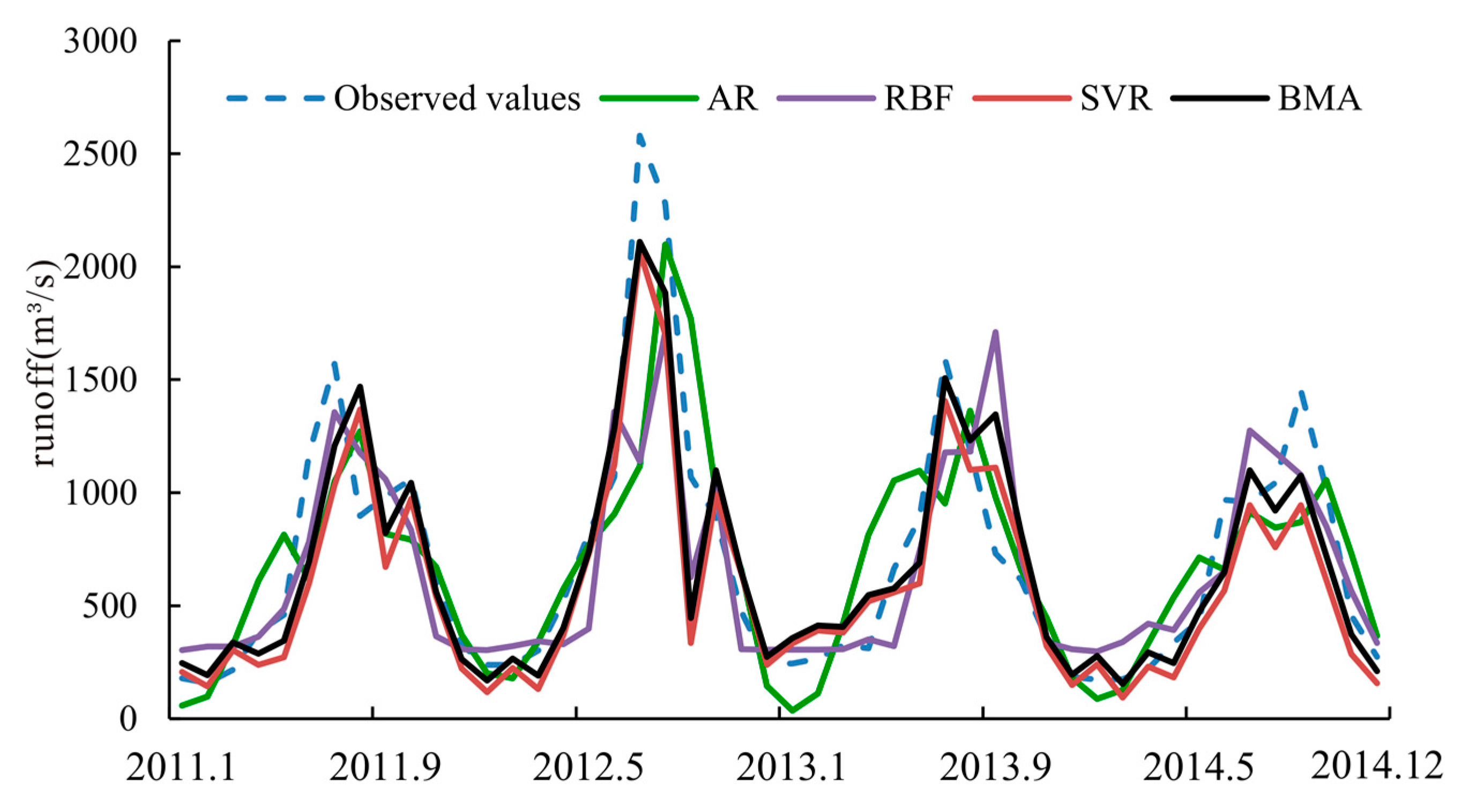
Figure 4 displays the comparison between predicted and observed runoff during model validation using MLR, RBFNN, SVR, and the BMA-based multimodel for Tangnaihai station. It can be seen that the SVR model obviously outperformed the MLR and RBFNN models during model validation in terms of the standard statistical measures (Table 2), and both the SVR and RBFNN models were able to forecast runoff. Specifically, the RMSEs for the SVR and RBFNN models were 274 and 327; the MAEs for the same two models were 0.250 and 0.307, respectively; their R² values were 0.905 and 0.798, respectively; and their NS values were 0.740 and 0.725, respectively. However, all of the other models performed better than the MLR model, which had the worst RMSE, MAE, R², and NS statistics, 296, 0.287, 0.777, and 0.697, respectively. Compared with all of the other models during model validation, the BMA-based multimodel obtained the best RMSE, MAE, R², and NS statistics, of 261, 0.196, 0.937, and 0.785, respectively. The classic MLR model is relatively easy to construct with the simplest type of parameters, and it can capture the global trend over an entire input space. Its accuracy, however, is not satisfactory, which may not meet the requirements of medium- and long-term runoff forecasting. The RBFNN model is capable of identifying complex nonlinear relationships between input and output data, and its accuracy is satisfactory for runoff forecasting, but there is a risk of over-fitting. The SVR model is also appropriate for reproducing the nonlinear problem, which can provide a suitable mapping between input and output data in a higher-dimensionality feature space to improve the forecasting accuracy. Its parameters need to be determined carefully due to the fact that they significantly influence the accuracy of the SVR model. Considering the overall characteristics of the above-mentioned models, the BMA-based multimodel significantly improves predictive performance.

4.3. High-Runoff Forecasting Analysis

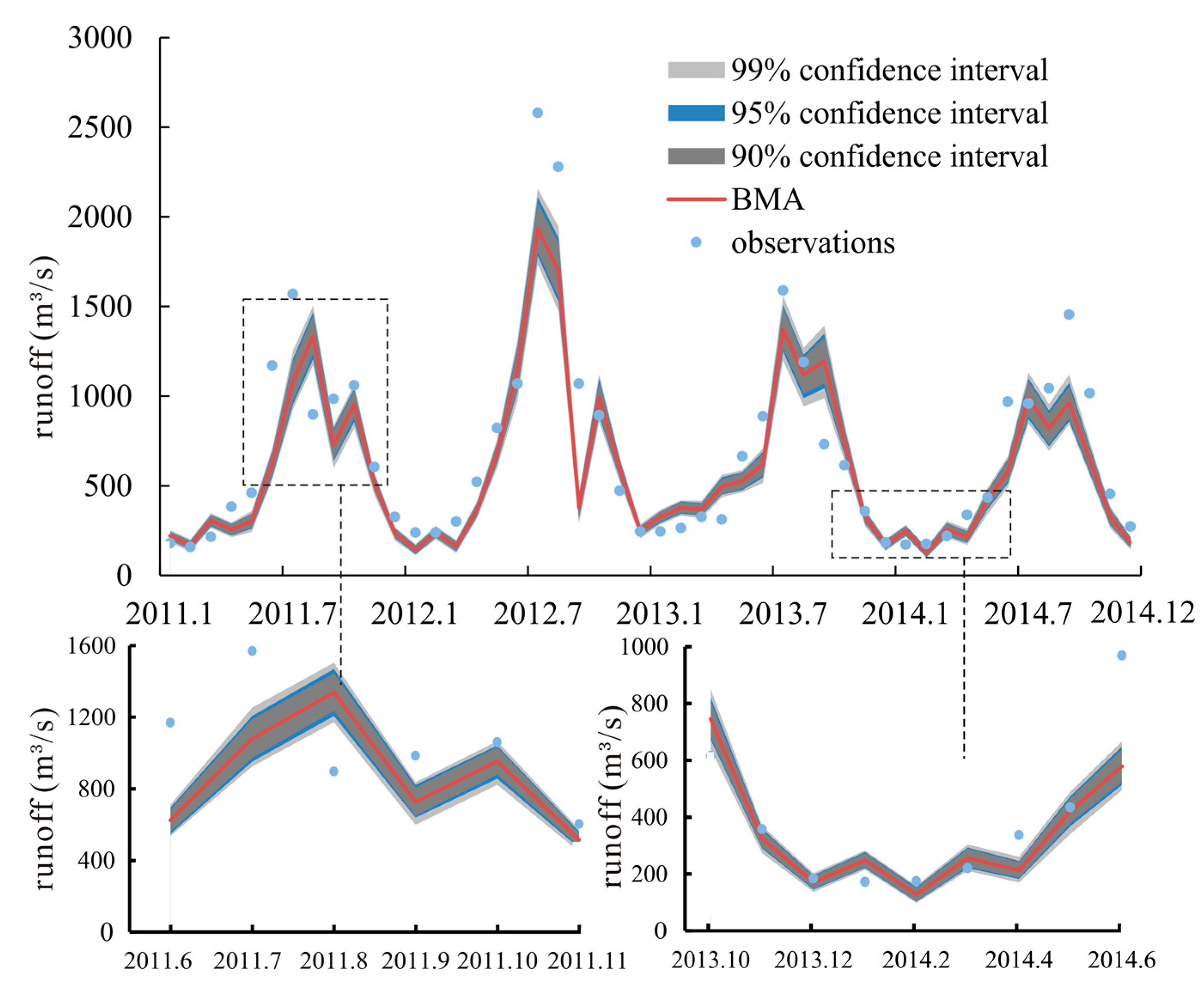
Figure 5 displays the results of BMA-based multimodel forecasting along with the 90%, 95%, and 99% confidence intervals. The performance of BMA confidence interval is evaluated by coverage ratio and interval width. As the confidence level gets higher, the corresponding confidence interval will be wider. Coverage ratio is the ratio of the number of points, which ranges between the confidence interval, to the number of total points. The larger the coverage ratio and the smaller the interval width are, the better the BMA model performs. Figure 5 shows that most of the observed values are within a 90% confidence interval. The coverage ratio can reach 80%, and the interval width is narrow in general, but most of the high-runoff observations are outside of the confidence interval, and the interval width is wider, which indicates the uncertainty of forecasting at high values is great.

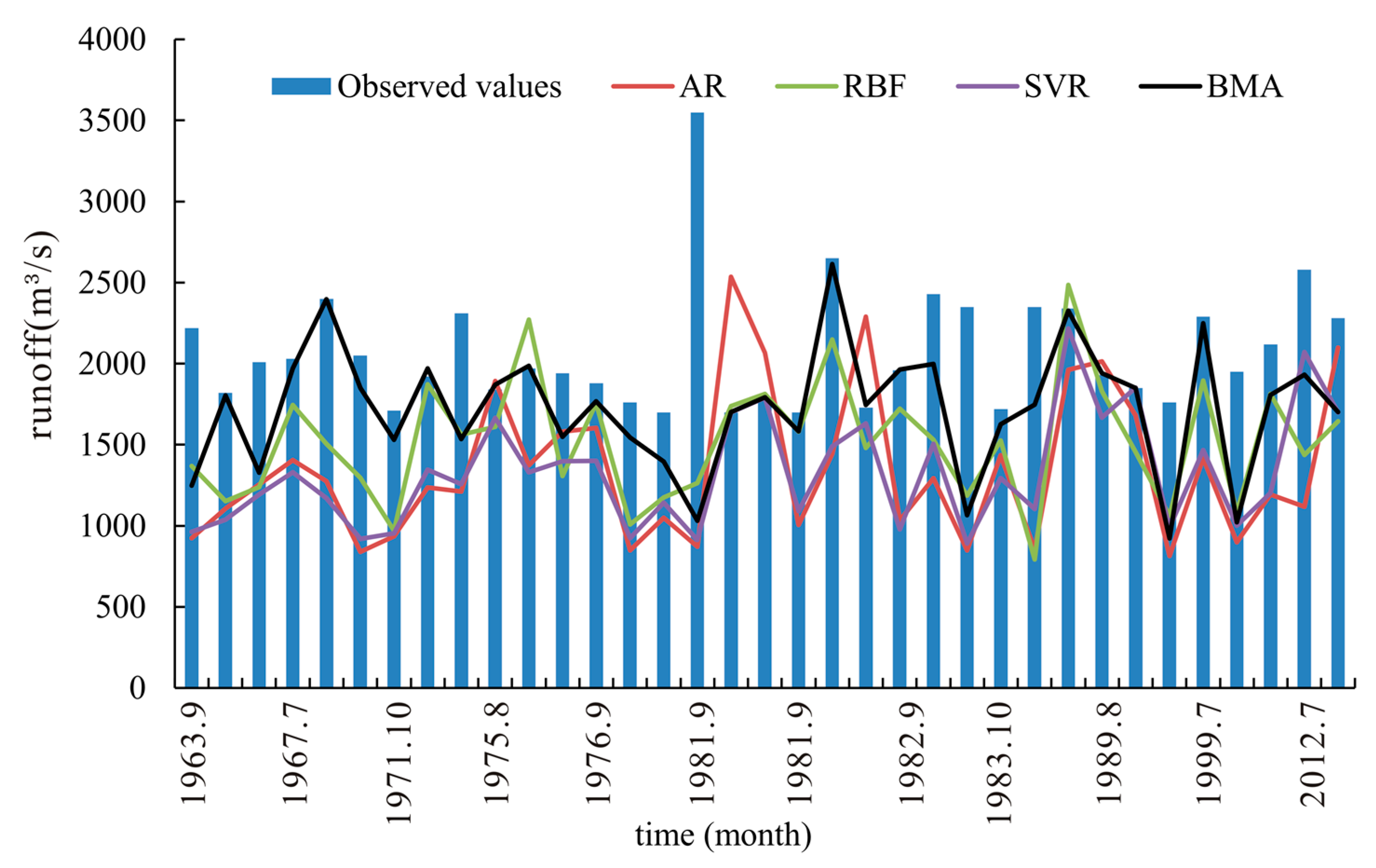
A runoff of over 1700 m³/s was selected to study the forecasting ability of high runoff for different models. The results are shown in Figure 6. The number of points used was 35, and the absolute differences between observed values and predicted values of all the points for different models were calculated. The minimal absolute differences for the BMA-based multimodel extended to 21 of 35 points, and the minimal absolute differences for the SVR, RBFNN, and MLR models extended to 5, 7, and 1 of 35 points, respectively. The BMA model has the best ability to forecast high runoff compared to all other models, the forecasting ability of the MLR model is the poorest, and the forecasting ability of the RBFNN and SVR models was better than that of the MLR model.

Generally, the BMA-based multimodel predicted values that are lower than the observed values when predicting high runoff. Since accurate prediction of extreme events would provide the most economic, environmental, and societal benefits, further improvements in high-runoff prediction are required.

There are significant differences between the observed values and the values predicted using all models for September 1981, and all of the models failed to capture extreme runoff events (3500 m³/s). The runoff in September 1981 was nearly two times greater than that for the same month in other years. Continuous rainfall occurred in the watershed above Tangnaihai station from August to September 1981, which resulted in serious flooding. As the major source of runoff, rainfall usually has the most significant impact on runoff, in addition, runoff also has a close relationship with evaporation, temperature, and other factors; although only the limited historical runoff time series available was applied in the paper, more runoff data needs to be considered for medium- and long-term runoff forecasting in the future.

Then another BMA-based multimodel was built for comparison based on only runoff time series. In the application, the first nine months of monthly runoff was used as the input, and the 10th monthly runoff as the output, details of validation samples were presented in

Table 3. Input-output pairs of runoff (m³/s) for model-validation process (without climatic factors).

Sample	Input (Runoff)									Output (Runoff)
1	317	373	1010	2120	945	689	617	422	203	179
2	373	1010	2120	945	689	617	422	203	179	158
3	1010	2120	945	689	617	422	203	179	158	216
4	2120	945	689	617	422	203	179	158	216	384
5	945	689	617	422	203	179	158	216	384	460
6	689	617	422	203	179	158	216	384	460	1170
…	…	…	…	…	…	…	…	…	…	…
42	29	274	116	580	17	18	20	1152	9	969
43	47	274	99	596	16	21	19	591	11	958
44	47	274	125	595	16	22	19	1788	10	1043
45	43	305	195	595	15	22	19	733	7	1454
46	18	236	253	576	16	21	19	223	1	1016
47	37	176	279	543	18	20	21	33	−4	455
48	20	89	301	521	19	18	22	83	−11	273

.

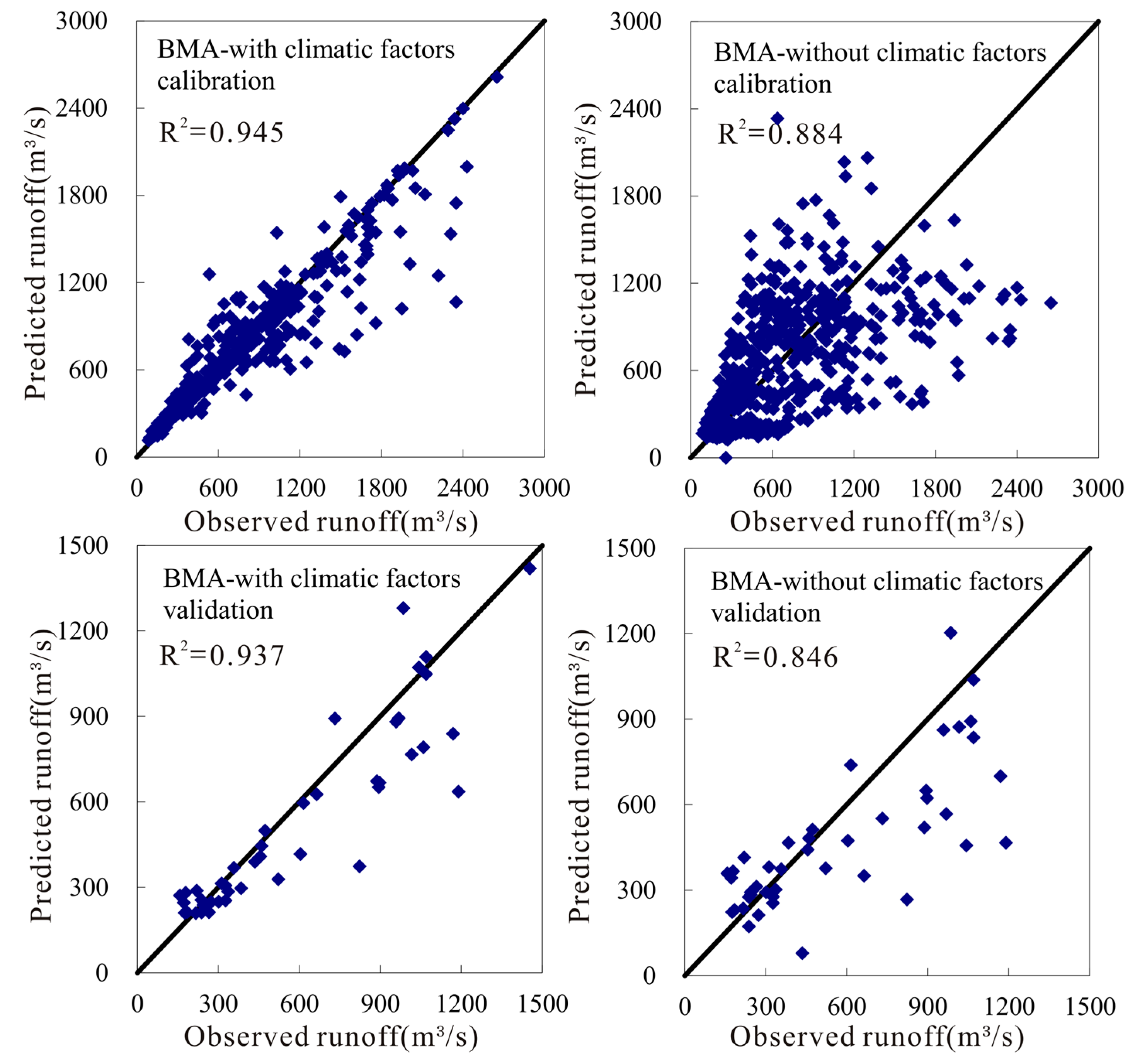
This displays the comparison between predicted and observed runoff using the BMA-based multimodel with and without climatic factors in Figure 7. Specifically, the R² for BMA-based multimodel, with climatic factors and without climatic factors, models were 0.945 and 0.884 during model calibration, and 0.937 and 0.846 during model validation, respectively. It can be seen that the BMA-based multimodel with climatic factors was generally superior to that without climatic factors during model calibration and validation. Large-scale oceanic–atmospheric conditions and local-scale climate indices have a direct or indirect influence on runoff variability in the source region of Yellow River, and it certainly improves medium- and long-term runoff forecasting with the linkage to different climatic factors.

5. Conclusions

The Yellow River headwater region is a headstream of other major rivers in China, and water resources are important for the surrounding area, so accurate runoff forecasting is of great significance for rational development and utilization of water resources. The monthly runoff data from Tangnaihai station in the Yellow River headwater region of China were analyzed as the case study. In this paper, under the full consideration of climatic factors, MLR, RBFNN, and SVR models were built for medium- and long-term runoff forecasting. The performance of the SVR model has changed significantly with different parameters. Hence, the main parameters of the models should be selected carefully. To further improve medium- and long-term runoff forecasting, a BMA-based multimodel was developed by the weighted sum of these aforementioned three models, and the forecasting results obtained using the BMA-based multimodel were compared to those obtained using the MLR, RBFNN, and SVR models during model calibration and validation. The results showed that the BMA-based multimodel obviously outperformed the RBFNN and MLR models during model calibration and validation. The BMA-based multimodel improved forecasting accuracy in terms of the standard statistical measures, and it also performed better for high-runoff forecasting than the other models, and gave forecasting results under the 90%, 95%, and 99% confidence intervals, respectively. In addition, the multimodel, with and without climatic factors, were built for comparison. However, the values predicted by the BMA-based multimodel are generally lower than the observed values when forecasting high runoff, and all of the models failed to capture extreme runoff events (3500 m³/s). Since accurate prediction of extreme events would provide the most economic, environmental, and societal benefit, further improvements in high-runoff prediction are required. Future research aimed at improving the forecasting model will take into consideration about some new approaches, such as deep learning model to build the complex nonlinear relationship between runoff and precipitation, temperature, and large-scale climate information.