Estimation of Sediment Yield Change in a Loess Plateau Basin, China

Abstract

Soil erosion is one of the most serious land degradation problems and the primary environmental issue in the Loess Plateau region of China. To identify the critical sub-basins and assess the impacts of land use change and climatic variability change on soil loss, this study tested the feasibility of the Soil and Water Assessment Tool (SWAT) model on sediment load simulation in the upper Sang-kan (USK) River basin. Based on a land use map of 1986, the SWAT model (Scenario 0) was calibrated at a monthly step using climate data from 1979 to 1985; then it was validated using climate data from 1986 to 1990. The monthly sediment simulation results indicated that the model did not work as well as streamflow simulation, indicating lower NS (Nash-Sutcliffe Efficiency) and r² values of 0.68, 0.69 and 0.61, 0.59 for the calibration period and validation period, respectively. This model could perform well under relatively low rainfall events, but it underestimated or overestimated the sediment load under high rainfall events. Comparing the results of scenarios with different land use maps (year of 1986 vs. 2012) and climate periods (1979–1990 vs. 2001–2012), it can be concluded that: (i) extreme and severe erosion almost always happened in FRST (forest land) and RNGE (grassland) in the hilly area; (ii) long-term traditional farming weakens the soil anti-erosion capability of land, leading to higher soil erosion, while forest can improve the soil structure, enhance the soil anti-erosion capability, and reduce soil erosion; (iii) both land use change and climatic change have led to the sediment yield decrease in the USK basin. Acting as the major influencing factor, land use change contributed to about 64.9% of the sediment yield reduction in the USK river basin.

1. Introduction

The Loess Plateau is an ecologically fragile zone in China and one of the areas most impacted by soil and water loss in the world due to its semi-arid climate, poor vegetation cover, and highly erodible loess soil [1,2,3]. This naturally fragile ecological system combined with long-term human activities that impact the environment (e.g., agricultural practices, urbanization, and deforestation) have resulted in land degradation, a water shortage, and continuous deterioration of the ecological environment, forming a vicious cycle [4,5,6]. The main soil erosion type in the Loess Plateau region is soil water erosion. Long dry periods followed by heavy bursts of intensive rainfall, falling on steep hilly slopes with fragile soils and low vegetation cover, expose this region to serious soil erosion risk. The soil loss from this region ranges from 20,000 to 30,000 t km⁻² yr⁻¹ [7]. This endangers food security and leads to major environmental and economic problems [8,9,10]. Removing topsoil that is rich in nutrients, soil erosion can also lead to a decline in soil productivity and soil biodiversity, which reduces the productive capacity of the land and restricts the growth of vegetation. Since the beginning of the 21st century, many ecological projects and measures, such as terrain construction, “Grain for Green” reforestation, and reclamation projects, have been implemented in order to change this situation. Downward trends of runoff and soil erosion have been detected and proved by many researchers in this region [2,7,11,12].

Soil erosion is a complex issue resulting from the mutual interaction of natural and human factors, irreversibly deteriorating soil quality. It is quantified by the average amount of soil removed from a defined area over a given time period [13,14]. Sediment yield is the amount of soil transported to rivers and lakes in a given period over a defined area, which is an important process in catchment soil erosion [6]. Among the factors influencing soil erosion, soil properties and topography are considered as constant factors in the short term, while some climatic variables (like daily rainfall, temperature, solar radiation, wind speed, etc.) and land cover types are the dominant influencing factors changing the erosion process in the short term [11,15,16,17]. Water and soil erosion is highly related to rainfall [1,3,16,17]. Especially in semi-arid regions, there is a marked relationship between rainfall and soil erosion. The amount of rainfall and maximum intensity have large effects on sediment losses: the amount of rainfall controls the removal of splash-generated loose soil particles and the maximum rainfall intensity determines the amount of soil splash. Generally, most soil loss occurs in high-intensity storm events [2,18,19]. Continuous surface runoff gathering can form rill erosion, gully erosion, and even gully erosion. These types of erosion erode and degenerate the farmland, and they are also the channel of runoff, sediment, and pollutant transport. In general, gully erosion in the active phase is the main source of soil loss in a watershed [20,21]. Land use, regarded as a concentrated reflection of human activity, is a significant dynamic parameter affecting the soil erosion process. Through altering the vegetation type and land cover, as well as the micro-topography, land use/cover influences the dynamic and resistant mechanisms of soil erosion [5,22]. The influences of land use and plant cover are considered the most important and, to some extent, exceed those of rainfall intensity and slope gradient on soil erosion [1,23,24]. Vegetation often reduces runoff and erosion due to its canopy, roots, and litter components [25]. Soil erosion and sediment yield are also two important indicators of environmental quality. Intensive soil erosion and excessive sediment indicate the loss of fertilizer and tillage layer, and destruction of farmland. Sediment deposition will reduce the water capacity of river channels and reservoirs, increasing the risk of flooding in rainstorms. In addition, reservoir siltation can cause the water quality to decline, causing an increased oxygen demand, accumulation of nutrients and pollutants, and increased turbidity, etc. Contaminated sediment, from the farmland, industrial sites, and residential zone, carries pollutants into rivers. Both of these lead to water ecosystem deterioration, and pose a threat to the survival of organisms in the reservoir and the drinking water safety [6,13]. In addition, the Loess Plateau is affected by both water erosion and wind erosion. Wind erosion in this area can also put large pressure on soil erosion. Wind speed is the primary factor influencing soil wind erosion. A higher wind speed leads to stronger erosion. With an arid to semiarid climate, the dry soils are more likely to be eroded [20,21].

Located on the Loess Plateau, the Sang-kan River, which is the headwater of the Yongding River, is upstream of the Dongyulin reservoir and the Guanting reservoir. The Sang-kan River basin is a large basin which involves four provincial administrative units, namely Shanxi Province, Inner Mongolia, Beijing, and Tianjin. This area is home to the Jinbei Coal Base, a pillar coal industry of China. With heavy mining and the coal industry rising, drastic land use change has been happening since 1985, with the elimination of vegetation and permanently altering topography, soils, and subsurface geological structures. In order to control the soil and water erosion and restore the ecosystem, a series of soil conservation practices, like terrace construction, “Grain for Green”, and Land Reclamation Projects, have been in operation since 1999. Due to the combination of climate change and human activities, most parts of the Sang-kan River have stayed in a situation of perennial drought since 1997. Sediment transported in this river has correspondingly decreased. Meanwhile, regional floods and serious erosion usually occur in the hilly areas or steep slopes covered with low woodland and grassland cover under rainstorm conditions. Therefore, a clear understanding of sediment yield and which areas are prone to high soil erosion can enable good land use planning and reservoir management, which can help to improve the ecological environment and ensure drinking water security in the capital.

Several erosion models used in the watershed scale have been developed and successfully applied in many regions around the world. The empirical ones mainly include the USLE and RUSLE model [26]. With the development of computer technology and the understanding of hydrological processes, distributed hydrological models (such as ANSWERS, EUROSEM, RUNOFF, KINEROS, EROSION3D, LISEM), and continuous distributed hydrological models (e.g., WEPP, SWAT, ACRU, MEDRUSH, etc.) have become powerful tools for streamflow and sediment assessment [26,27,28,29]. Among the numerous hydrologic models that have been developed in recent years, the Soil and Water Assessment Tool (SWAT) excels, with several advantages over other models, including multiple functions, a modular design, and only a few parameters. Therefore, SWAT has become one of the most suitable models not only for hydrological simulations, but also for the assessment of sediment and nutrient transport at a watershed scale worldwide [29,30,31]. In recent years, SWAT has been applied to successfully simulate sediment yields and transport in a few studies of China [6,10,32,33,34]. In this study, SWAT was applied to the upper Sang-kan (USK) river basin, which is used as an example of catchments located in the Loess Plateau region that suffer from both drought and soil erosion. The objectives of this study were to: (i) evaluate the performance of SWAT for sediment simulation in the USK basin using monthly data; (ii) calibrate and validate the model to provide a sound basis for the sediment simulation under different land use and climate scenarios; and (iii) detect the areas of severe soil erosion.

2. Materials and Methods

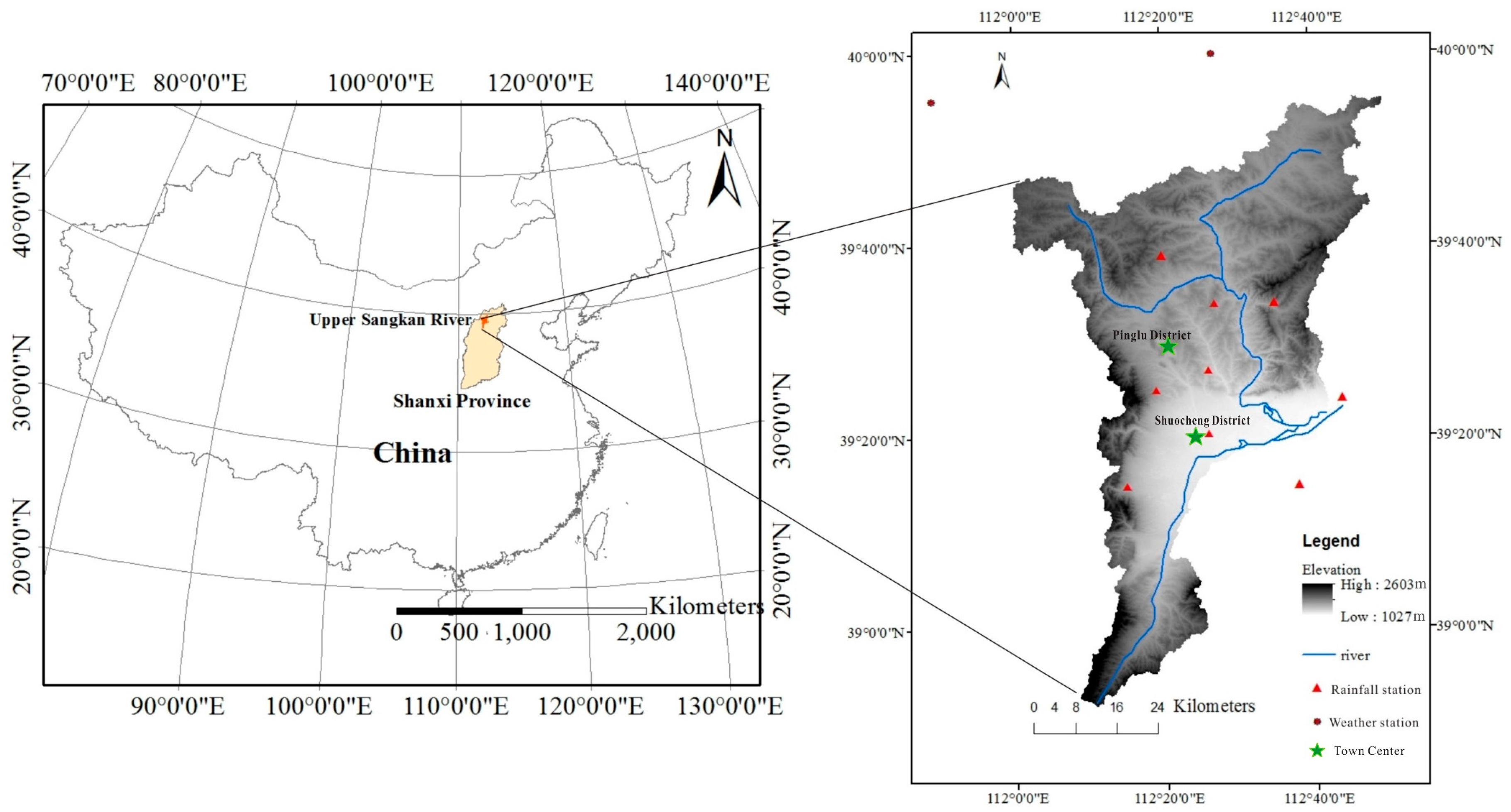
2.1. Study Watershed

The upper Sang-kan (USK) basin, located in the Loess Plateau area of Shanxi Province, China, was chosen as the study area. To avoid the influence of the reservoir (constructed in 1994) on river flow, the USK basin located in the upstream region was selected. The drainage area of the USK basin is around 3430 km², with geographic coordinates of 112°10′58′′–113°30′ E, 38°51′–39°55′ N (Figure 1).

The length of the USK River is around 124 km. The northeast-southwest alignment of mountains structures the terrain. The terrain characteristics of this region are complex and the geomorphology is diverse. Elevation of this basin ranges from 1027 m at the watershed outlet to 2602 m in the hilly region. The hilly region is mainly located in the north, and the alluvial lacustrine plain is distributed in the southern and eastern part. Vegetation in this region is sparse, and gully erosion is severe with a gully bed depth stretching from 30 m to 50 m, forming a typical Loess Plateau landscape. This area has a typical arid to semi-arid climate, with temperature and precipitation unevenly distributed throughout the year. Meanwhile, windward slopes are more frequent than leeward slopes in this region. Both make this study area a water-wind erosion crisscross region. The average annual precipitation is from 380 mm to 465 mm, with approximately 70–80% occurring from July to September. The annual mean temperature range is from 5.1 °C to 7.1 °C, with a higher temperature in the southeastern and central part and lower values in the hilly region. The average annually effective evaporation, however, is approximately 1152.1 mm, which is almost three times greater than the amount of precipitation [12,36]. Loess soil is widely distributed in this region. The physical weathering of soil is strong, and the soil texture tends to be sandy. Around 48% of this area is occupied with agricultural land, growing wheat, maize, millet, oats, etc. [25,37].

2.2. Modeling Approach

2.2.1. The SWAT Model

The Soil and Water Assessment Tool (SWAT 2012) is a process-based, distributed-parameter, agro-hydrological model, which can simulate streamflow and sediment for long periods of time at a daily time step at the watershed scale [30]. It was developed to predict the impact of land use and land management practices on water, sediment, and agricultural chemical yields in large watersheds [38]. Embedded within a geographical information system (GIS), the SWAT system can integrate various spatial data including climate, soil, land cover, and topographical features. Based on a digital elevation model [35] and the stream network, SWAT analyzes watersheds by delineating them into sub-basins. Then, the sub-basins are further subdivided into hydrologic response units (HRUs) that are assumed to be spatially uniform in terms of soil, land use, and topographic characteristics.

2.2.2. Hydrologic Modelling

Climatic variables including precipitation, temperature, solar radiation, wind speed, and relative humidity are the input drivers of the hydrologic cycle. They can be observed in a time series or simulated by a weather generator. Hydrologic processes taken into account in the HRUs include vadose zone processes (i.e., infiltration, evaporation, plant uptake, lateral flows, and percolation) and groundwater flows [30]. The hydrologic cycle simulation in SWAT is divided into two phases: the land phase and the water phase [38]. The simulation of the land phase is calculated from each HRU separately based on the water balance equation (Equation (1)).

$$S{W}_t=S{W}_0+{\displaystyle \sum }_{i=1}^t\left(R_{day}-Q_{surf}-E{T}_i-W_{seepi}-Q_{gw}\right)$$

(1)

where SW_t is the final soil water content, SW₀ is the initial soil water content, t (days) is the time, R_day is the precipitation on day i, Q_surf is the surface runoff on day i, ET_i is the evapotranspiration on day i, W_seepi is the amount of water entering the vadose zone from the soil profile on day i (soil interflow), and Q_gw is the amount of return flow on day i.

Runoff from the HRUs is measured to calculate the amount of water reaching the main channel in each sub-basin [38]. As for the water phase of the hydrologic cycle, SWAT uses a variable storage coefficient method or the Muskingum routing method to describe the routing of runoff in the river channel [39,40].

2.2.3. Suspended Sediment Modelling

SWAT calculates the sediment yield within each HRU using the Modified Universal Soil Loss Equation (MUSLE) [41], a modified version of the Universal Soil Loss Equation (USLE) developed by Wischmeier and Smith [42]. In MUSLE, the rainfall energy factor is replaced with a runoff factor, a function of antecedent moisture condition and rainfall energy, to simulate erosion and the sediment yield. This improves the accuracy of the sediment yield prediction, eliminates the need for delivery ratios, and enables sediment yields of single storms to be calculated. The MUSLE equation is:

$$sed=11.8·{\left(Q_{surf}\times q_{peak}\times are{a}_{hru}\right)}^{0.56}\times K_{USLE}\times C_{USLE}\times P_{USLE}\times L{S}_{USLE}\times CFRG$$

(2)

where sed is the sediment yield on a given day (metric tons), Q_surf is the surface runoff volume (mm/ha), area_hru is the area of the HRU (ha), K_USLE is the soil erodibility factor, C_USLE is the cover and management factor, P_USLE is the support practice factor, LS_USLE is the topographic factor, and CFRG is the coarse fragment factor.

Sediment transport from the sub-basin outlets to the basin outlet consists of two processes: deposition, which occurs when the upland sediment load is larger than the transport capacity of the channel; and degradation, which occurs when it is smaller. The amount of sediment finally reaching the basin’s outlet, S_OT, is given as:

$$S_{OT}=S_{IN}-S_D+D_T$$

(3)

where S_IN is the amount of sediment entering the reach, S_D is the amount of sediment deposited, and D_T is the total amount of sediment degradation, which is the sum of re-entrainment and bed degradation components. It is given as:

$$D_T=\left(D_r+D_B\right)\left(1-D_R\right)$$

(4)

where D_r is the sediment re-entrainment, D_B is the bed material degradation, and D_R is the sediment delivery ratio [38].

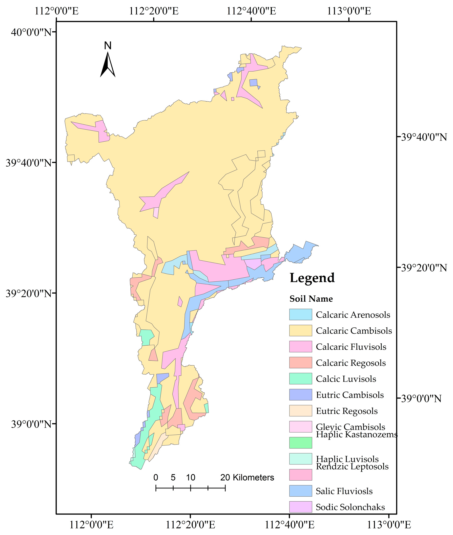
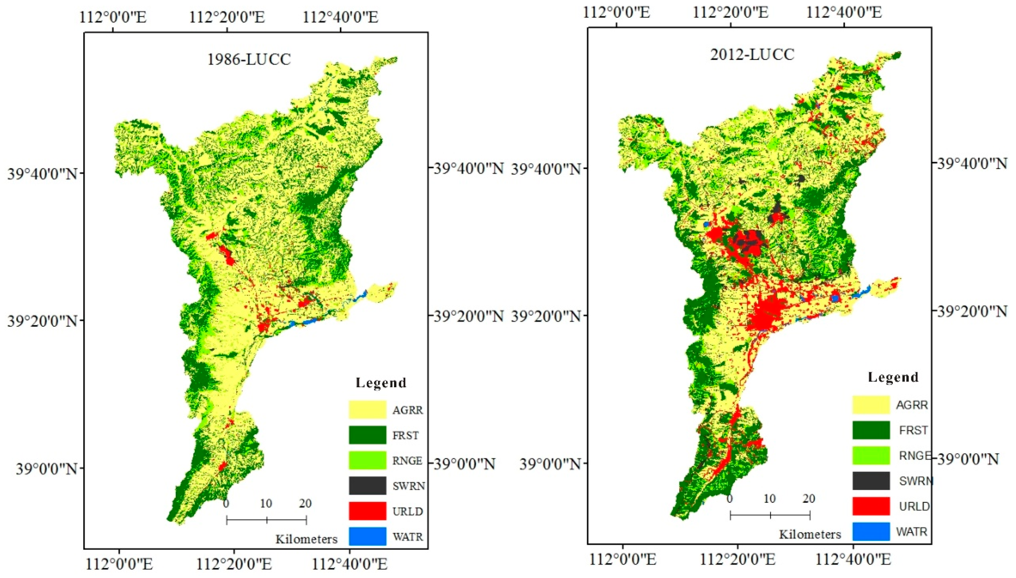
2.3. SWAT Input Data

Topographic, soil, land use, and hydro-meteorological data are required for the SWAT model setup. They were collected or generated as follows (

Table 1. The input data in the SWAT model.

Data Type			Data Format	Data Source	Application Modules
Spatial data	DEM		Grid	Geospatial Data Cloud	Runoff, interflow, Watershed delineation, river system generation
	Land use map		Grid/Shape	Interpreted from Landsat images via United States Geological Survey	Watershed subdivision, HRUs division
	Soil map		Grid/Shape	Harmonized World Soil Database (HWSD) and China soil database	HRUs division, Soil database
Attribute data	Climate data	Precipitation	txt	China Water Year Book	Evapotranspiration, runoff
		Maximum & minimum temperature, solar radiation, humidity, wind speed	txt	China Meteorological Data Sharing Service System; Global Weather Data for SWAT
	Hydrological data		txt	China Water Year Book	Ground water, Model calibration and validation
	Soil physical and chemical properties		DBF	HWSD and China soil database	Runoff, interflow

): The 30-m resolution DEM (1986) was downloaded from the Geospatial Data Cloud (http://www.gscloud.cn/) and spliced by ArcGIS. The soil properties database was established based on the connection of the Harmonized World Soil Database (HWSD) (http://www.fao.org/data/en/) and the China soil database. Soil properties, namely, the percentage of sand, clay, gravel, salinity, and organic matter, were taken from HWSD directly. Moreover, other soil properties, like the soil texture, available water, saturated hydraulic conductivity, and matric bulk density, were calculated by SPAW (soil-plant-air-water), which is a soil water characteristics software that was developed by Washington State University, USA (http://hydrolab.arsusda.gov/soilwater). The spatial distribution of soil types is shown in Figure 2. Using ENVI (Environment for Visualizing Images), land use maps of 1986 and 2012 were interpreted from Landsat images in September, downloaded via the United States Geological Survey (http://glovis.usgs.gov/) (Figure 3.) The classification of land use types is displayed in

Table 2. The classification of land use types in the upper Sang-kan (USK) river basin.

Land-Use Type	Meaning	SWAT Code
Agriculture land	Terrace land, Slope farmland, etc.	AGRR
Forest land	Shrub land, newly planted young forest, mixed forest of coniferous and broad-leaved forest, broad-leaved forest, protection forest for cultivated land, etc.	FRST
Grassland	Artificial grassland, grassland, protection grassland for cultivated land	RNGE
Unused land	Bare land, non-reclaimed mining dump land	SWRN
Building land	Village and urban construction land, roads, etc.	URLD
Water body	Reservoir, river, channel, etc.	WATR

Notes: AGRR, Agricultural land with row crops; FRST, Mixed forest; RNGE, Range-grasses; SWRN, Southwestern US (arid) range; URLD, Residential land in low density; WATR, Water.

.

Two sets of observed daily meteorological data (taking out the rainfall data) were used in this study (Table 1). One set of climate data (1979–1990 and 2001–2012) which includes the maximum and minimum temperature, solar radiation, humidity, and wind speed data, was from two weather stations outside of the study area (Wuzhai and Youyu), downloaded from the China Meteorological Data Sharing Service System (http://data.cma.cn/). To improve the accuracy of the climate input, another set of daily meteorological data within the basin was downloaded from Global Weather Data for SWAT (http://globalweather.tamu.edu/). Water and soil erosion is highly related to rainfall. To ensure the quality of rainfall data and the final simulation results, we used the precipitation data observed at nine rainfall stations inside this study basin. Daily precipitation (1979–1990 and 2001–2012) at the rainfall stations and daily stream discharge data and sediment concentration data (1981–2012) at one hydrologic station were collected from the China Water Year Book. The nine rainfall stations are Gaoyu, Dangjiagou, Yuling, Xiaoyinzhuang, Haoxiaofeng, Liujiayao, Wangwanzhuang, Fushanzhuang, and Dongyulin, and the hydrologic station is Dongyulin station.

2.4. Model Calibration and Validation

ArcSWAT (18 October 2012), an ArcGIS extension and graphical user input interface for SWAT 2012, was used in this present study to delineate the boundaries of the entire study area and its sub-basins. Based on the soil map, the land use map of 1986, and climate data from 1979 to 1990, the SWAT model was set up. Finally, the USK basin was divided into 21 sub-basins and 358 HRUs with a threshold area of 9000 ha. The entire simulation period was divided into the calibration period (1981–1985) and the validation period (1986–1990). For calibration and validation, the initial two years were considered as a warm up period and the simulated outputs of these two years were discarded to minimize the effect of user estimated parameter values [43]. Then, the modeling output run at a monthly time step was compared with the observed monthly average streamflow and sediment data at Dongyulin station.

SWAT input parameters are physically based and are allowed to vary within a realistic uncertainty range for calibration [44]. The auto-calibration and uncertainty analysis for this research was performed using the Sequential Uncertainty Fitting Program (SUFI-2) in the SWAT-CUP package [45,46]. SWAT-CUP 2012 (SWAT Calibration and Uncertainty Programs) is an interface developed for SWAT. Being easily linked to SWAT, it can perform sensitivity analysis, calibration, validation, and uncertainty analysis. Parameter uncertainty in SUFI-2 accounts for all sources of uncertainties in the driving variables (e.g., rainfall), parameters, conceptual model, and measured data (e.g., observed flow and sediment). The parameter uncertainty is described by a multivariate uniform distribution in a parameter hypercube, while the output uncertainty is quantified by the 95% prediction uncertainty band (95 PPU) calculated at the 2.5% and 97.5% levels of the cumulative distribution function of the output variables. All sources of uncertainty are mapped to a set of parameter ranges. The percentage of data bracketed by the 95% prediction uncertainty (95 PPU) band (P-factor) and a measure of the average width of the 95 PPU (R-factor) were used to quantify the goodness of calibration-uncertainty performance. No exact numbers exist for what these two factors should be, but values of >70% for P-factor and an R-factor of around 1 are generally suggested [46].

2.5. Model Evaluation

The performance of the model in the sediment simulation was evaluated by Nash-Sutcliffe Efficiency (NS) and the Coefficient of Correlation (r²). The equations are as follows in Equations (5) and (6) [47,48]:

$$NS=1-{\displaystyle \sum }_{i=1}^n{\left(Q_{obs}-Q_{sim}\right)}^2/{\displaystyle \sum }_{i=1}^n{\left(Q_{obs}-mean\left(Q_{obs}\right)\right)}^2$$

(5)

where Q_obs and Q_sim are the measured and simulated data, respectively, and n is the total number of data records. As NS approaches 1, the model simulates the measured data more accurately. Generally, NS is very good when NS is larger than 0.75, satisfactory when NS is between 0.36 and 0.75, and unsatisfactory when NS is lower than 0.36. When NS is negative, the model is a worse predictor than the measured mean [47,49].

$$r^2={\left[{\displaystyle \sum }_{i=1}^n\left(Q_{obs,i}-{\overline{Q}}_{obs}\right)\left(Q_{sim,i}-{\overline{Q}}_{sim}\right)\right]}^2/{\displaystyle \sum }_{i=1}^n{\left(Q_{obs,i}-{\overline{Q}}_{obs}\right)}^2{\displaystyle \sum }_{i=1}^n{\left(Q_{sim,i}-{\overline{Q}}_{sim}\right)}^2$$

(6)

where Q_obs and Q_sim are the measured and simulated data, and i is the ith measured or simulated datum. As with NS, as r² approaches 1, the model simulates the measured data better.

2.6. Sensitivity Analysis

A global sensitivity analysis in SWAT-CUP was used to identify parameter sensitivity, which was calculated by the following multiple regression system (Equation (7)) [46]. It regresses the Latin hypercube generated parameters against the objective function value:

$$g=\alpha +{\displaystyle \sum }_{i=1}^m{\beta }_i{b}_i$$

(7)

where b_i is the parameter and m is the number of parameters for analysis. α and β are the regression coefficients. A t-test is used to identify the relative significance of the parameters. The sensitivities are estimates of the average changes in the objective function resulting from changes in each parameter, while all other parameters are changing. The t-stat is the coefficient of a parameter divided by its standard error. The p-value for each term tests the null hypothesis that the coefficient is equal to zero (no effect). In this analysis, the larger, in absolute value, the value of t-stat, and the smaller the p-value, the more sensitive the parameter.

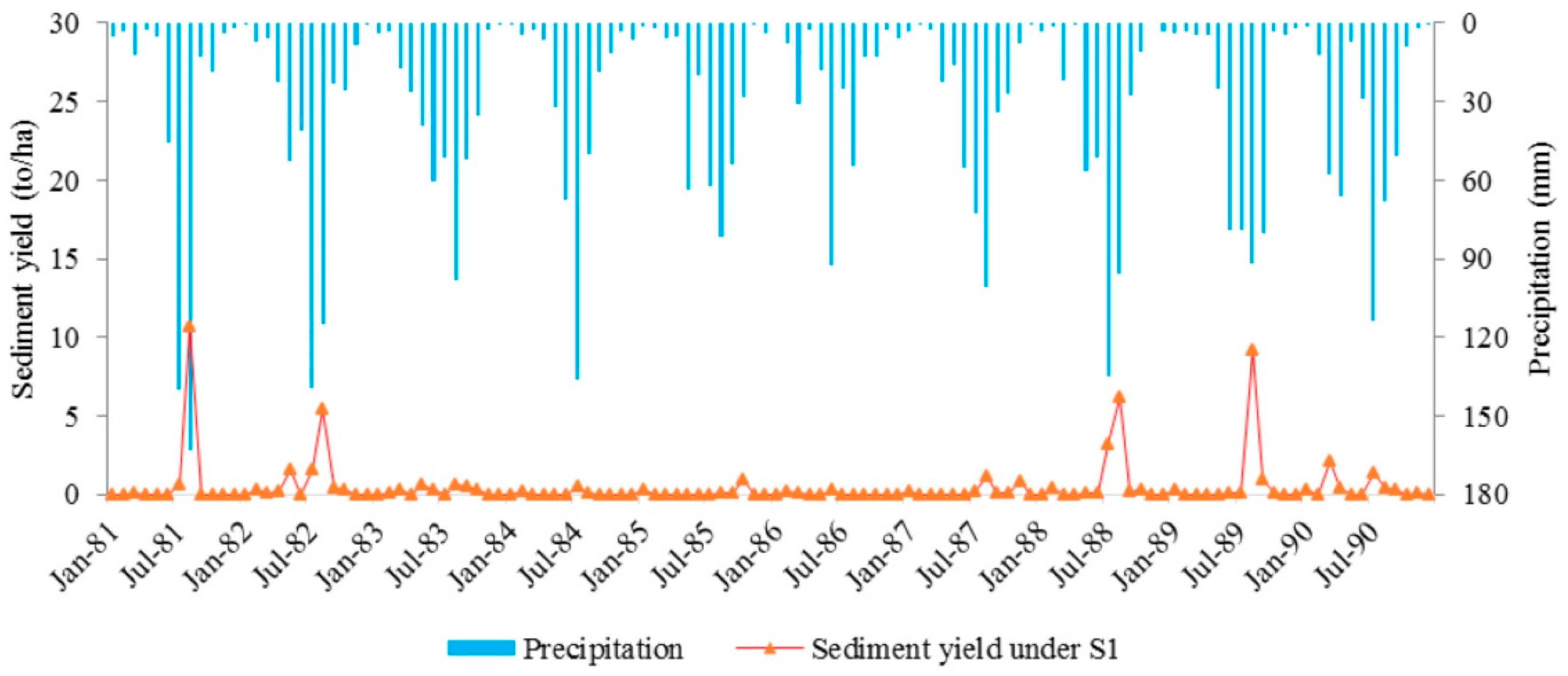
2.7. Scenario Analysis

The approach of one factor at a time was used based on the calibrated SWAT model to evaluate the effect of climatic variability and land use change on the sediment yield. Considering the availability of the climate and hydrologic data and the construction of the reservoir, meteorological data from 1981 to 1990 were selected as the “baseline period” without too much human interference, and the period from 2001 to 2012 was selected as the “human impact period” with the interference of the reservoir and other human activities. The land use maps of 1986 and 2012 were used to represent the land use patterns of the two time-slices. Then, the calibrated SWAT model under Scenario 0 (S0) was run for each of the two combinations of these two time-slices and two land use maps. The influences of land use change and climatic variability were quantified by comparing the SWAT outputs of the three scenarios as follows:

• Scenario 0 (S0): climate data from 1979 to 1990 and land use of 1986.
• Scenario 1 (S1): climate data from 1979 to 1990 and land use of 2012.
• Scenario 2 (S2): climate data from 2001 to 2012 and land use of 2012.

3. Results and Discussions

3.1. Watershed Characteristics

The most widespread soil class in the USK basin is Calcaric Cambisols, consisting of 21% clay, 43% silt, and 36% sand, (Figure 2). Figure 3 displays the land use types and their area coverage in 1986 in the USK river basin. The land use classes are agricultural land (AGRR) 54.4%, forestland (FRST) 26.9%, grassland (RNGE) 15.4%, unused land (SWRN) 1.0%, building land (URLD) 1.9%, and water body (WATR) 0.4%. According to the natural river network and the topography of the basin, the USK basin was divided into 21 sub-basins. In order to obtain a reasonable resolution of soil properties, land use, and management practices, the threshold value of land use, soil type, and slope were chosen as 10%, 3%, and 7%, respectively.

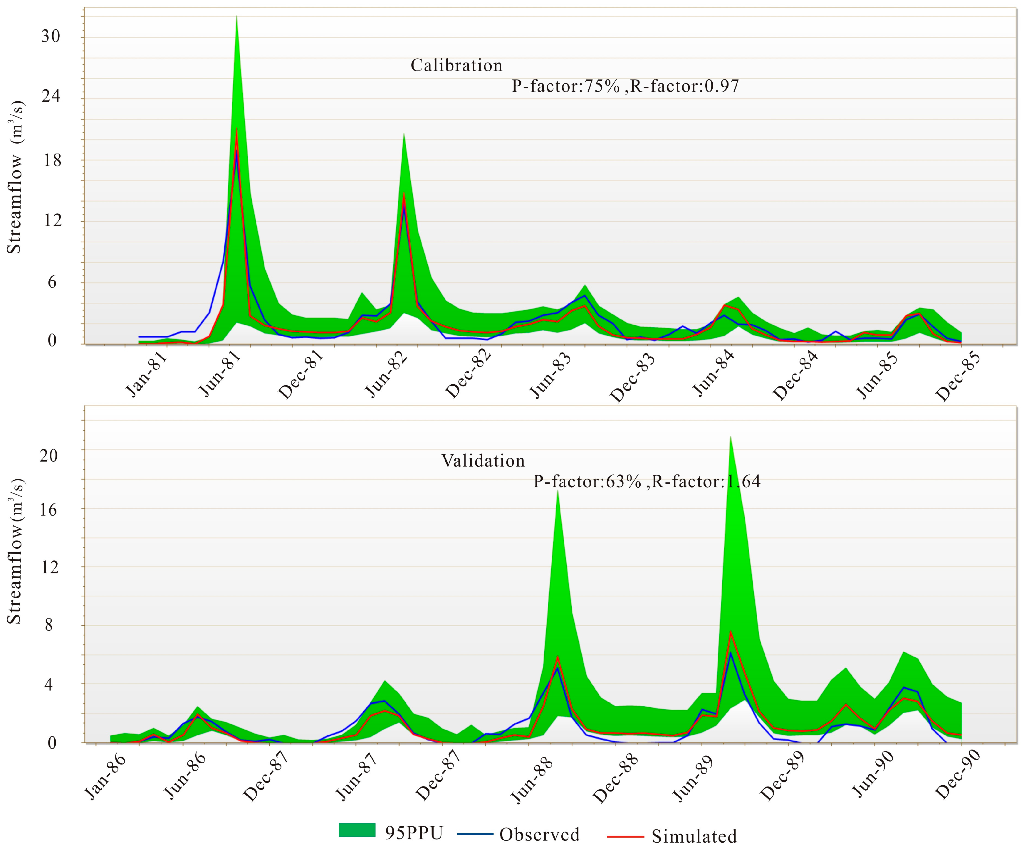
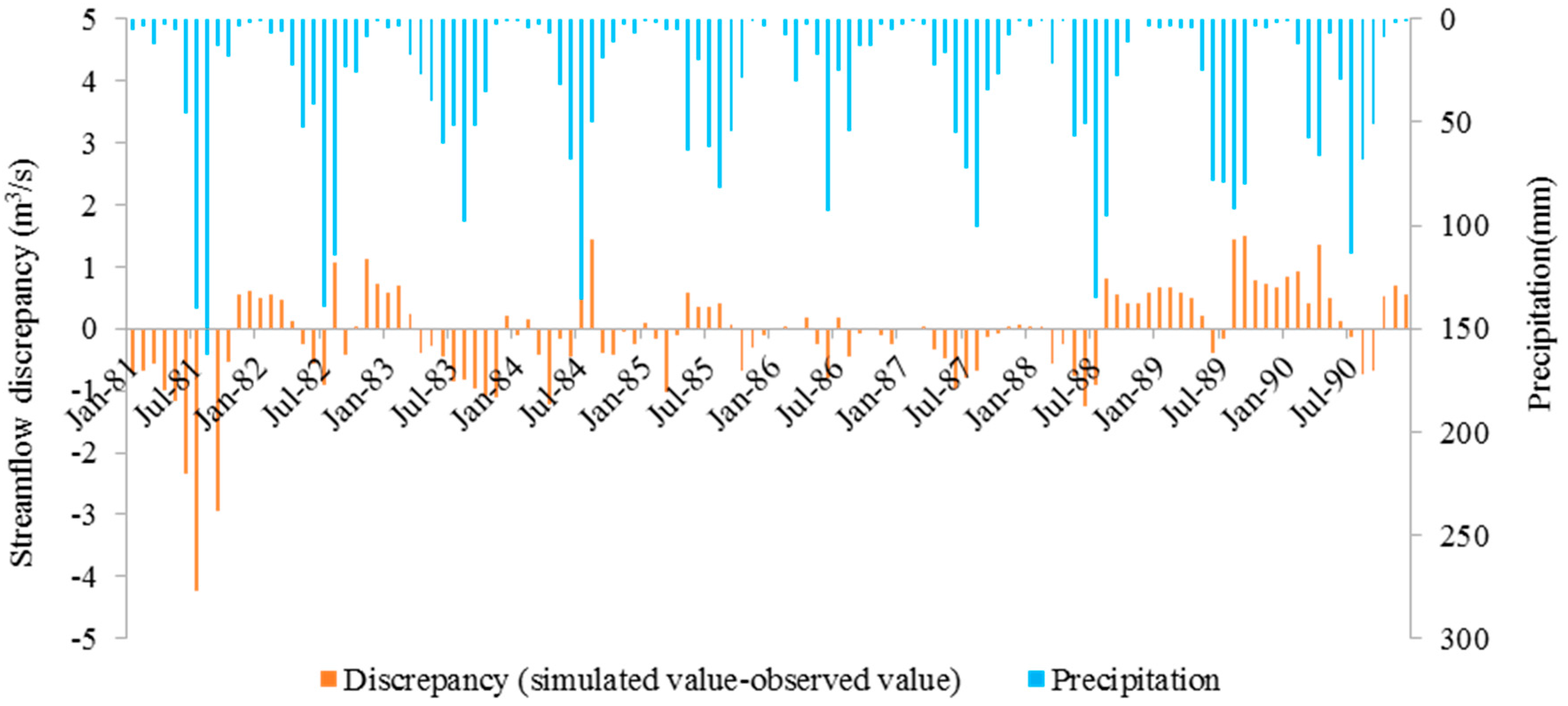
3.2. Evaluation of the Streamflow Simulation

A list of sensitive parameters in SWAT for the study area are given in

Table 3. List of sensitive parameters calibrated based on global sensitivity analysis.

Order	Parameters	Meaning	Best Parameters	t-Stat	p-Value
1	CN2 RO	Curve number	−7.36% r	37.00	0.000
2	USLE_C{2} SD	Min value of USLE C factor applicable to FRST	0.44	17.31	0.000
3	SLSUBBSN SD	Average slope length	181.97	6.79	0.000
4	SOL_AWC RO	Available water capacity of the soil layer	−20.36% r	−5.91	0.000
5	REVAPMN RO	Threshold depth of water in the shallow aquifer for “revap” to occur (mm)	326.5	1.86	0.064
6	SPEXP SD	Exponent parameter for calculating sediment re-entrained in channel sediment routing	1.18	1.65	0.098
7	USLE_C{3} SD	Min value of USLE C factor applicable to RNGE	0.38	1.64	0.101
8	GW_DELAY SD	Groundwater delay (days)	368.12	1.5	0.133
9	CANMX RO	Maximum canopy storage	13.23	−1.47	0.141
10	CH_COV1 SD	Channel erodibility factor	0.34	−1.33	0.184
11	SPCON SD	Linear parameter for calculating the maximum amount of sediment that can be reentrained during channel sediment routing	0.01	−1.28	0.202
12	GW_REVAP RO	Revap coefficient	0.07	−0.94	0.348
13	ALPHA_BF RO	Base-flow recession constant	0.46	0.86	0.392
14	SOL_K RO	Saturated hydraulic conductivity (mm/h);	+19.78% r	0.49	0.625
15	CH_COV2 SD	Channel cover factor	0.03	−0.49	0.625
16	CH_N2 RO	Manning’s “n” value for the main channel	0.10	0.46	0.648
17	EPCO RO	Plant uptake compensation factor	0.51	0.42	0.675
18	CH_ERODMO SD	Jan~Dec. channel erodability factor	0.24	−0.34	0.731
19	ESCO RO	Soil evaporation compensation coefficient	0.24	0.28	0.778
20	RCHRG_DP RO	Deep aquifer percolation fraction	0.59	0.27	0.786
21	CH_K2 RO	Effective hydraulic conductivity in main channel (mm/h)	174.49	0.20	0.841
22	USLE_C{1} SD	Min value of USLE C factor applicable to AGRR	0.05	−0.195	0.84
23	GWQMN RO	Treshold depth of water in the shallow aquifer required for return flow to occur (mm).	580.48	0.03	0.973

Notes: ^RO means the parameters related to streamflow calibration; ^SD means the parameters related to sediment calibration; ^r means the relative change of initial value.

. Thirteen parameters marked with “^RO” in Table 3 were chosen for calibration of the streamflow simulation [50,51,52]. With the automatic calibration approach of SUFI-2 in SWAT-CUP, the NS value and r² value are 0.89 and 0.91, and the P-factor and R-factor are 75% and 0.97, respectively; for the validation dataset, the NS value is 0.79 and the r² value is 0.82, and the P-factor and R-factor are 63% and 1.64, respectively. The results indicated good agreement between the simulated and measured monthly streamflow values both in the calibration period and the validation period.

As shown in Figure 4 and Figure 5, the timing and the recession of streamflow peaks are simulated reasonably in most cases, with some simulation delay in the summer of 1984, 1987, 1988, and 1989. In addition, the maximum flow of most peaks was underestimated and the streamflow during the low-flow periods was overestimated. This discrepancy has a strong link to the observed climate data. Heavy rainfall events in remote parts of the catchment were not captured by the climate stations, leading to underestimations of streamflow peaks. Another possible reason for this discrepancy is that the present curve number (CN) technique cannot accurately predict runoff for days that experience several storms. The soil moisture level and the corresponding runoff curve number vary from storm to storm. However, when several storms occur in a single day, SCS-CN methods define a rainfall event as the sum of all rainfall that occurs in a whole day, which might lead to an underestimation of runoff [53,54]. On the other hand, the overestimations of streamflow during low-flow periods might be caused by the higher parameterization value of CN2 [32].

3.3. Sensitivity Analysis of Sediment Parameters

Keeping the values of the streamflow parameters unchanged, another 10 parameters affecting the sediment load, marked with “^SD”, were added for the sediment simulation, as shown in Table 3 [10,55,56,57,58]. The results of the global sensitivity analysis on sediment parameters are listed based on their ranking (Table 3). It shows that CN2, USLE_C {2}, SLSUBBSN, SOL_AWC, REVAPMN, SPEXP, USLE_C {3}, GW_DELAY, CANMX, and CH_COV1 are the 10 highest sensitivity parameters for sediment simulation. Curve number-“CN2” and the minimum value of the USLE_C factor applicable to FRST—“USLE_C {2}” are much higher than the others, ranked in first and second place, indicating that they are the most important and most sensitive parameters. Only two parameters (CH_COV1 and SPEXP) concerning channel erodibility rank in the top 10 highly sensitive parameters, indicating that the overall sediment yield is assumed to be more sensitive to overland erosion, whereas channel erosion is presumed to be of minor importance. An accurate estimation of these parameters is important for a sediment simulation with the SWAT model in the USK river basin. Then, these parameters were adjusted from the SWAT initial estimates to fit the model simulations with the observed streamflow and sediment concentration data. These parameters and their calibrated values are displayed in Table 3.

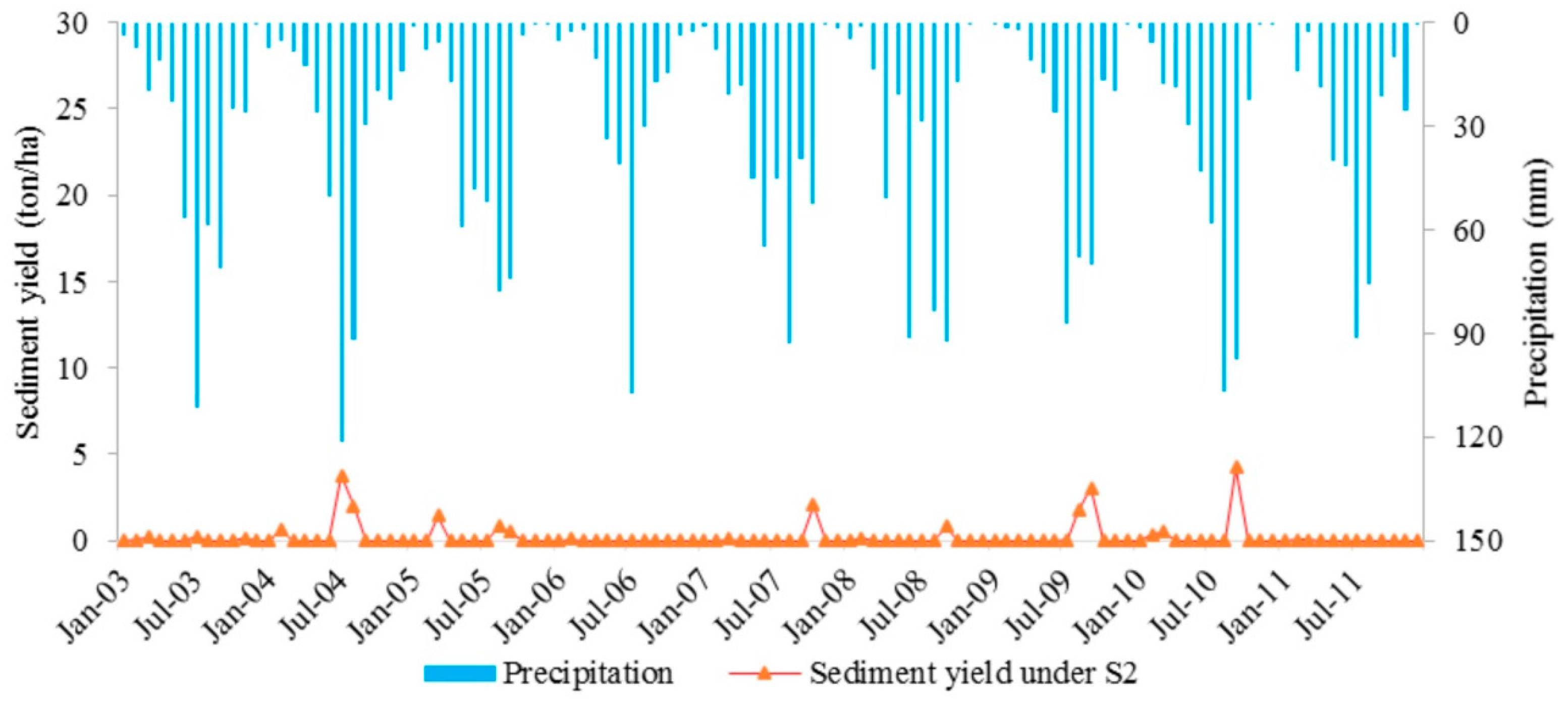
3.4. Evaluation of Sediment Load Simulation

The values of NS (0.68), r² (0.69), P-factor (64%), and R-factor (0.61) demonstrated that the agreement between the simulated and observed sediment was acceptable for model calibration. For the validation period, the NS, r², P-factor, and R-factor values were 0.61, 0.59, 57%, and 0.53, respectively. The model evaluation statistics indicated an accordingly low model performance for the sediment simulation, especially for the validation period. Although the simulated monthly sediment yields were generally in agreement with the measured values, the model performance during all 10 years of the calibration and validation periods is considerably lower than the observed performance (Figure 6). The SWAT model tends to underestimate sediment loads for high rainfall events while overestimating sediment loads for low rainfall events (Figure 6). Runoff simulation impacts measurement uncertainties and uncertainties in model parameterization, and errors or oversimplifications inherent in the model structure can be responsible for this mismatch [32,59]. In this basin, sediment simulation uncertainty is mainly introduced by the observed data used for model calibration and validation. The recorded sediment loads might be underestimated because short-term events were not captured by the sampling, or they might be overestimated because high loads measured during short-term events are extrapolated to whole days. Measurement errors might be introduced for the choice of an unrepresentative sampling location or during laboratory analyses [10,60]. Another reason for this poor sediment simulation effect is that the study area is in the wind-water erosion crisscross region and the wind erosion has some impact on the total soil erosion value; however, the SWAT model is developed based on water erosion without the simulation of wind erosion processes. As a result, the absence of a scientific wind erosion simulation in the SWAT model combined with the influence factors mentioned above resulted in poor simulation results.

3.5. Spatial Distribution of Soil Loss under Different Land Use Scenarios

3.5.1. Sediment Yield under Scenario 0

Assessment of the spatial variability of soil erosion in the Loess Plateau is very useful for catchment management planning and land use management. According to the gradation of the soil erosion standard in the Loess Plateau of China, the soil erosion level in this basin was classified into six grades (

Table 4. The distribution of different erosion grades of HRUs in sub-basins under Scenario 0.

Soil Erosion Grades		Soil Erosion Modulus	The Sub-Basins of HRUs Locating	Area (km2)
				FRST	RNGE	AGRR	Total
Extreme		>150 t ha−1 yr−1	18, 19	34.6	10.4	0	45
severe		80–150 t ha−1 yr−1	7–9, 19, 21	12	3	0	15
strong		50–80 t ha−1 yr−1	4, 7–9, 18–21	53.3	47.2	0	100
moderate		25–50 t ha−1 yr−1	3, 4, 6–9, 12, 17–21	94.7	64.9	0	159.7
low		10–25 t ha−1 yr−1	2–9, 11–13, 17–21	180.6	99.3	64.4	344.3
slight	slight-III	10–5 t ha−1 yr−1	1–9, 11–13, 17, 18, 19–21	283.2	105.8	236.5	625.5
	slight-II	2–5 t ha−1 yr−1	1–3, 6–17, 19–21	44.84	64	559.1	667.9
	slight-I	<2 t ha−1 yr−1	1–21	257.4	96.9	1090	1444

): slight (0–10 t ha⁻¹ yr⁻¹), low (10–25 t ha⁻¹ yr⁻¹), moderate (25–50 t ha⁻¹ yr⁻¹), strong (50–80 t ha⁻¹ yr⁻¹), severe (80–150 t ha⁻¹ yr⁻¹), and extreme (>150 t ha⁻¹ yr⁻¹). The sediment yield in this region is not that serious, based on the gradation of the soil erosion standard because a large amount of eroded soil may be deposited during transportation. Therefore, the slight grade was subdivided into three sub-gradations: 0–2 t ha⁻¹ yr⁻¹; 2–5 t ha⁻¹ yr⁻¹; and 5–10 t ha⁻¹ yr⁻¹ to distinguish the erosion differences. The HRUs with extreme, severe, and strong erosion were in sub-basins 4, 7–9, and 18–21, with areas of 45 km², 15 km², and 100 km², respectively; HRUs with moderate erosion were mainly in sub-basins 3, 4, 6–9, 12, and 17–21, with an area of 159.7 km²; the low eroded HRUs were mainly in sub-basins 2–9, 11–13, and 17–21, with an area of 344.3 km²; while HRUs with slight erosion occurred in all the sub-basins, with the largest total area of 2737 km². It can be concluded that in the hilly area, the moderate to extreme eroded HRUs mainly occurred in the FRST and RNGE, while most slight and low eroded HRUs were distributed on the agricultural land (AGRR). The soil erosion extent of the 21 sub-basins under Scenario 0 (S0) in the USK basin is shown in Figure 7. There were no extreme or severe average erosions at the sub-basin scale under S0. Sub-basin 18 experienced an overall strong erosion, and sub-basin 19 experienced an overall moderate erosion. Low erosion mainly occurred in sub-basins 3, 4, and 6. The rest of the sub-basins only exhibited slight soil loss. The soil erosion degree of different land use types in the sub-basins under S0 are displayed in

Table 5. The soil erosion gradation of different land use in sub-basins of the USK river basin from 1986 to 2012.

Sub-Basin	Land Use 1986 under S0						Land Use 2012 under S1
	AGRR	FRST	RNGE	SWRN	URLD	WATR	AGRR	FRST	RNGE	SWRN	URLD	WATR
1							−1		-
2								−1	-		-
3								−1	+1
4								−1	-
5							−1	−1	-
6								−1	+1
7								−1	+1	-
8								−1
9							+1
10								−1		-	-
11										-	-
12							+1	+1	-		-
13							+2	+1	-		-
14
15							−1	-
16							+1				-
17							+1				-
18							+1
19							+1
20							−1		−1		-
21							−1	−1	-

Notes: “ ” means the severe soil erosion level, “ ” means the strong soil erosion level, ” ” means the moderate soil erosion level, “ ” means the low soil erosion level, “ ” means the slight soil erosion level; in the right part of the table, the data of “+1” and “+2” mean the soil erosion level increased by one or two level comparing with that of 1986, while “−1” means the soil erosion level decreased by one level. “-” means new land use types with no comparison.

. Extreme erosion occurred in the agricultural land use in sub-basins 14 and 15 and the forest land use in sub-basin 21.

The observed average sediment yield at the outlet of the USK basin was 219 × 10⁴ t yr⁻¹. The SWAT model simulation result under S0 was 204 × 10⁴ t yr⁻¹, a little lower than but close to the observed data.

3.5.2. Sediment Yield under Scenario 1

Under Scenario 1 (S1), this basin was divided into 380 HRUs and 21 sub-basins. No HRUs had extreme soil erosion; severe and strong eroded HRUs were located in sub-basins 18 and 19, with areas of 325.1 km² and 386.4 km², respectively; some HRUs in sub-basins 3, 6, 8, 18, 19, and 21 were predicted to have moderate erosion, with a total area of 842.9 km²; low eroded HRUs were predicted to occur in sub-basins 3–9 and 18–21, with an area of 703.7 km²; while slight eroded HRUs had a total area of 723.7 km² (

Table 6. The distribution of different erosion grades of HRUs in sub-basins under Scenario 1.

Soil Erosion Grades		Soil Erosion Modulus	The Sub-Basins of HRUs Locating	Area (km2)
				FRST	RNGE	AGRR	Total
Extreme		>150 t ha−1 yr−1	-	0	0	0	0
severe		80–150 t ha−1 yr−1	19	92.3	232.9	0	325.1
strong		50–80 t ha−1 yr−1	18, 19	119.3	267.1	0	386.4
moderate		25–50 t ha−1 yr−1	3, 6, 8, 18, 19, 21	396.7	446.2	0	842.9
low		10–25 t ha−1 yr−1	3–9, 18–21	248.5	455.2	0	703.7
slight	slight-III	10–5 t ha−1 yr−1	1–9, 11–13, 17, 18, 19–21	196.1	110.3	37.5	343.9
	slight-II	2–5 t ha−1 yr−1	1–3, 6–17, 19–21	100.1	66.3	120.8	287.2
	slight-I	<2 t ha−1 yr−1	1–21	35.9	12.2	44.5	92.6

). Similar to S0, the moderate to severe erosion of HRUs was predicted to happen in the forest and grassland. At a sub-basin scale, no sub-basin experienced moderate to extreme soil loss (Figure 7). Only sub-basins 18, 19, and 21 exhibited low erosion, while the rest of the sub-basins had different grades of slight erosion. The soil erosion gradation of different land use types in the sub-basins under S1 are displayed in Table 5. It can be concluded that the areas prone to severe levels of erosion were the agricultural land in sub-basins 14, 16, and 17.

The sediment yield results predicted by SWAT were 190 × 10⁴ t yr⁻¹ under S1, which was 14 × 10⁴ t yr⁻¹ less than the simulation results of S0. The sediment yield rate had decreased from 11.1 t ha⁻¹yr⁻¹ to 5.6 t ha⁻¹yr⁻¹ during 1986 to 2012. Therefore, land use change caused the sediment yield to reduce by 49.7%.

3.5.3. Impact of Land Use Change on Spatial Sediment Yield Distribution

It can be seen from

Table 7. The area change of land use in sub-basins of the USK river basin from S0 to S1.

Sub-Basin	AGRR Area (km2)	FRST Area (km2)	RNGE Area (km2)	SWRN Area (km2)	URLD Area (km2)	WATR Area (km2)	SYLD Change Rate (t ha−1 yr−1)	Erosion Rate Decrease Order
1	−55.7	2.0	52.8	0.0	0.0	0.0	0.7	21
2	−17.6	−9.9	10.8	0.0	13.6	0.0	−0.8	12
3	3.2	−16.1	13.4	0.0	0.0	0.0	0.2	18
4	−10.9	−8.9	20.2	0.0	0.0	0.0	−3.7	8
5	−2.2	−0.8	3.0	0.0	0.0	0.0	0.5	20
6	−11.1	0.5	10.6	0.0	0.0	0.0	−0.4	14
7	−13.5	−1.1	3.8	11.2	0.0	0.0	−6.1	6
8	−8	3.1	4.9	0.0	0.0	0.0	−9.1	5
9	−17.9	13.6	4.9	0.0	0.0	0.0	−12.0	3
10	−43.8	4.6	0.73	16.1	22.9	0.0	0.4	19
11	−73.4	22.5	−14	20.8	44.4	0.0	−1.1	11
12	−17.6	32.5	−33.8	0.0	19.1	0.0	−2.1	10
13	−4.8	−1	−30.8	0.0	37.0	0.0	−2.7	9
14	−0.4	0.0	0.0	0.0	0.0	0.3	0.01	15
15	−33.3	8.7	0.0	0.0	24.9	0.0	0.2	17
16	0.3	−2.9	0.0	0.0	6.5	−3.9	0.1	16
17	−10.8	−10.3	−7.7	0.0	28.9	0.0	−0.5	13
18	4.1	8.0	−12.1	0.0	0.0	0.0	−44.5	1
19	−19.3	32.1	−12.4	0.0	0.0	0.0	−25.2	2
20	−46.6	23.5	0.5	0.0	22.6	0.0	−5.9	7
21	−46.9	22.3	24.4	0.0	0.0	0.0	−10.8	4
Total	−426.2	122.7	39.2	48.0	219.9	−3.5	−5.5

Note: SYLD means the sediment yield.

that except in sub-basins 1, 3, 5, 10, 14, 15, and 16, the majority of sub-basins in this study area had different grades of sediment yield decrease. Sediment yielded from hilly sub-basin 18 had the highest decrease rate (44.5 t ha⁻¹ yr⁻¹), because grassland (RNGE) was transformed into forest land (FRST) and agricultural land (AGRR). FRST exceeds RNGE at soil protection. With developed roots and a thicker canopy and litter layers, forests have better water infiltration, surface soil protection, and surface runoff reduction, which will decrease soil erosion [25]. Due to the construction of terraces in the hilly area, the runoff and soil eroded from the agricultural land can be intercepted by the field ridge, which can also have a good effect on soil and water protection during the rest period. Ranking in second place, sub-basin 19 had a decrease rate of 25.2 t ha⁻¹ yr⁻¹, which was probably caused by the change of farmland and grassland to forest land; altering agricultural land back to forest and grassland in the hilly area had a good effect on the soil erosion reduction in sub-basins 9 and 21. The increase in soil erosion in hilly sub-basin 1 and sub-basin 5 was mainly induced by the transformation of agricultural land (AGRR) to grassland (RNGE). Without artificial management and protection, the grassland degraded gradually which aggravated soil erosion; a large area of agricultural land (AGRR) occupied by the extension of unused land (SWRN) and construction land (URLD) increased the soil loss from sub-basin 10; the decrease of forest land (FRST) in the hilly area resulted in the increase of erosion in sub-basin 3. The high-intensity exploitation of coal resources and the development of resource industries, as well as the vegetation deterioration, land excavation, surface subsidence, etc., in this process made the soil erosion in sub-basins 10 and 15 increase.

Severe soil erosion occurred in agricultural land (AGRR) in the plain area, and strong soil erosion mostly appeared in forest land (FRST) and agricultural land (AGRR) (Table 5). From 1986 to 2012, the area of agricultural land (AGRR) experienced a heavy decline of 426.2 km²; the construction land (URLD) witnessed a rapid expansion, increasing by 219.9 km²; the forest land (FRST), grassland (RNGE), and unused land (SWRN) increased by 112.7 km², 39.2 km², and 48.0 km², respectively (Table 7). As displayed in Table 5, the soil erosion degree of agricultural land in sub-basins-14, 15, 16, and 17 in the plain area increased. This is because the sediment erosion simulation in the SWAT model was based on the traditional tillage system. Without straw covering, the rainfall strikes the loose plowed soil directly, which makes the soil particles easy to be broken and the clay soil generated in this process will fill the soil channel, making a surface crust and hardened layer. As a result, the water infiltration will be blocked, increasing the runoff and soil erosion [61]. However, with the development of a tillage system, new methods like residue cover, no till, subsoiling, etc., were introduced gradually as conservation tillage in this study basin in recent years. This kind of conservation tillage system can improve soil capillary and soil aggregate structure, increasing water infiltration and soil anti-erosion capability and decreasing soil and water erosion. However, without the consideration of this tillage change on soil erosion, the SWAT model overestimated the soil erosion in the agricultural land in the plain area. Additionally, the soil loss from most of the forest land reduced. It can be concluded that forest had an obvious positive effect on soil conservation. With a thicker canopy, forest can decrease the direct strike of rainfall on land surface and intercept a large amount of precipitation. The litter layers of forest will increase the surface roughness and the capacity of holding water. With developed roots, a forest can improve the soil structure and soil anti-erosion capability, leading to better water infiltration and reducing water and soil erosion [25].

3.6. Spatial Distribution of Sediment Yield under Different Climate Scenarios

In order to assess the impact of climate change on sediment yield, the simulation results of Scenario 1 (S1) and Scenario 2 (S2) were compared. Hydrological systems can be very sensitive to climate changes, particularly in arid and semi-arid regions [62]. Hydrological processes in these kinds of arid regions are strongly affected by precipitation and temperature. Surface runoff generally shows a good positive correlation with annual rainfall in this Losses Plateau region [7]. Warming temperatures will lead to higher evapotranspiration and a decline in runoff, which is the driving force of soil erosion [63]. Therefore, climate change can have a great influence on soil erosion. With the same land use of 2012, the average air temperature of S2 increases from 5.8 °C to 6.1 °C, while the average annual precipitation declines by 5.7 mm compared to S1. The monthly temperature and precipitation from 1986 to 2012 are shown in Figure 8. S2 tends to experience warmer and drier summers (from Jun to Aug), which prevents extremely high streamflow and soil erosion in the rainy seasons (Figure 8). The sediment yield responses to different climate scenarios are shown in Figure 9. The sediment yields from the sub-basins under S2 are displayed in Figure 7, and sediment yields from the sub-basins under different scenarios are shown in

Table 8. The rate of sediment yield in the USK river basin during 1986–2012.

Sub-Basin		SYLD (t ha−1 yr−1)		Sub-Basin		SYLD (t ha−1 yr−1)
	Scenario 0	Scenario 1	Scenario 2		Scenario 0	Scenario 1	Scenario 2
1	1.6	2.3	0.6	12	2.9	0.9	0.3
2	3.5	2.7	0.9	13	3.5	0.8	0.4
3	5.7	5.9	2	14	0.03	0.04	0.02
4	9.7	6	2.5	15	0.6	0.7	0.5
5	4.5	5	2.3	16	0.05	0.1	0.1
6	5.6	5.2	1.5	17	0.1	0.5	0.4
7	11	4.9	2.1	18	60.7	16.2	2.8
8	16.2	7	3.1	19	41.9	16.7	3.5
9	19.3	7.3	5.1	20	11.7	5.8	8
10	1	1.4	0.6	21	21.3	10.5	15.7
11	2.1	1.1	0.5	Average	11.1	5.6	2.6

Note: SYLD means the sediment yield.

.

Both the average monthly sediment yield from the whole basin and the annual sediment yield from the outlet of this basin decreased from S1 to S2. Climate change from 1986 to 2012 in the USK basin resulted in the rate of sediment yield decreasing from 5.6 t ha⁻¹ yr⁻¹ to 2.6 t ha⁻¹ yr⁻¹, and the overall amount of sediment yield decreased from 192 × 10⁴ t yr⁻¹ to 89 × 10⁴ t yr⁻¹. Land use change caused the sediment yield rate decrease from 11.1 t ha⁻¹ yr⁻¹ to 5.6 t ha⁻¹ yr⁻¹, contributing to about 64.9% of the sediment yield decline from 1986 to 2012.

4. Conclusions

Although the modelled sediment yields did not perform as well as the streamflow, the simulated and measured sediment yields are still in reasonable agreement.

• The simulation results showed that both the land use change and climate change in these years led to the decrease in sediment yield.
• The extreme and severe erosion mostly occurred in the hilly area.
• Forest land and terraces are confirmed to have a better effect on erosion reduction in this area.
• Long-term traditional tillage will weaken the soil anti-erosion capability of land, leading to higher soil erosion. Forest, on the other hand, can improve the soil structure, enhance the soil anti-erosion capability, and have a large positive effect on soil conservation.
• Acting as the major influencing factor, land use change caused about 64.9% of the sediment yield reduction in the USK basin.

Some processes, like gully erosion, wind erosion, and tillage methods change, are not included in the SWAT model and are not reflected in model parameterization at the sub-basin or HRU level. It is difficult to post an outside experiment and build a gully erosion model or tillage methods, and then embed them in SWAT as modules. The wind-water crisscrossed erosion only happened in the northwest part of the study region, which can only have a limited influence. In addition, with multiple functions and only a few required parameters, the SWAT model helps us solve the problem of the paucity of data. The overall advantages of using the SWAT model overweigh its disadvantages. In addition, the former successful SWAT application in the Loess Plateau region added strength to this current study. Therefore, this modelling approach could be helpful for understanding the causes of sediment yield change in the USK basin and gives relative estimates of the erosion measure, enabling scientific land use planning and catchment management for a better ecological environment.

References

1. Sun, W.; Shao, Q.; Liu, J. Soil erosion and its response to the changes of precipitation and vegetation cover on the loess plateau. J. Geogr. Sci. 2013, 23, 1091–1106. [Google Scholar] [CrossRef]
2. Kang, S.; Zhang, L.; Song, X.; Zhang, S.; Liu, X.; Liang, Y.; Zheng, S. Runoff and sediment loss responses to rainfall and land use in two agricultural catchments on the loess plateau of china. Hydrol. Process. 2001, 15, 977–988. [Google Scholar] [CrossRef]
3. Liu, L.; Liu, X.H. Sensitivity analysis of soil erosion in the northern loess plateau. Procedia Environ. Sci. 2010, 2, 134–148. [Google Scholar] [CrossRef]
4. Mosbahi, M.; Benabdallah, S.; Boussema, M.R. Assessment of soil erosion risk using swat model. Arab. J. Geosci. 2012, 6, 4011–4019. [Google Scholar] [CrossRef]
5. Sun, W.; Shao, Q.; Liu, J.; Zhai, J. Assessing the effects of land use and topography on soil erosion on the loess plateau in china. Catena 2014, 121, 151–163. [Google Scholar] [CrossRef]
6. Ouyang, W.; Hao, F.; Skidmore, A.K.; Toxopeus, A.G. Soil erosion and sediment yield and their relationships with vegetation cover in upper stream of the yellow river. Sci. Total Environ. 2010, 409, 396–403. [Google Scholar] [CrossRef] [PubMed]
7. Li, C.; Qi, J.; Feng, Z.; Yin, R.; Guo, B.; Zhang, F.; Zou, S. Quantifying the effect of ecological restoration on soil erosion in china’s loess plateau region: An application of the mmf approach. Environ. Manag. 2010, 45, 476–487. [Google Scholar] [CrossRef] [PubMed]
8. Lal, R. Soil degradation by erosion. Land Degrad. Dev. 2001, 12, 519–539. [Google Scholar] [CrossRef]
9. Jain, M.K.; Das, D. Estimation of sediment yield and areas of soil erosion and deposition for watershed prioritization using gis and remote sensing. Water Resour. Manag. 2009, 24, 2091–2112. [Google Scholar] [CrossRef]
10. Bieger, K.; Hormann, G.; Fohrer, N. Simulation of streamflow and sediment with the soil and water assessment tool in a data scarce catchment in the three gorges region, china. J. Environ. Qual. 2014, 43, 37–45. [Google Scholar] [CrossRef] [PubMed]
11. Chen, L.; Huang, Z.; Gong, J.; Fu, B.; Huang, Y. The effect of land cover/vegetation on soil water dynamic in the hilly area of the loess plateau, china. Catena 2007, 70, 200–208. [Google Scholar] [CrossRef]
12. Fu, B.; Zhao, W.; Chen, L.; Zhang, Q.; Lü, Y.; Gulinck, H.; Poesen, J. Assessment of soil erosion at large watershed scale using rusle and gis: A case study in the loess plateau of china. Land Degrad. Dev. 2005, 16, 73–85. [Google Scholar] [CrossRef]
13. Tripathi, M.P.; Panda, R.K.; Raghuwanshi, N.S. Identification and prioritisation of critical sub-watersheds for soil conservation management using the swat model. Biosyst. Eng. 2003, 85, 365–379. [Google Scholar] [CrossRef]
14. Sutherland, R.A.; Ziegler, A.D. Effectiveness of coir-based rolled erosion control systems in reducing sediment transport from hillslopes. Appl. Geogr. 2007, 27, 150–164. [Google Scholar] [CrossRef]
15. Marques, M.J.; Bienes, R.; Jimenez, L.; Perez-Rodriguez, R. Effect of vegetal cover on runoff and soil erosion under light intensity events. Rainfall simulation over usle plots. Sci. Total Environ. 2007, 378, 161–165. [Google Scholar] [CrossRef] [PubMed]
16. Croke, J.; Nethery, M. Modelling runoff and soil erosion in logged forests: Scope and application of some existing models. Catena 2006, 67, 35–49. [Google Scholar] [CrossRef]
17. Koiter, A.J.; Owens, P.N.; Petticrew, E.L.; Lobb, D.A. The role of soil surface properties on the particle size and carbon selectivity of interrill erosion in agricultural landscapes. Catena 2017, 153, 194–206. [Google Scholar] [CrossRef]
18. Sadeghi, S.H.R.; Sharifi Moghadam, E.; Khaledi Darvishan, A. Effects of subsequent rainfall events on runoff and soil erosion components from small plots treated by vinasse. Catena 2016, 138, 1–12. [Google Scholar] [CrossRef]
19. Wen, L.; Zheng, F.; Shen, H.; Bian, F.; Jiang, Y. Rainfall intensity and inflow rate effects on hillslope soil erosion in the mollisol region of northeast china. Nat. Hazards 2015, 79, 381–395. [Google Scholar] [CrossRef]
20. Jiang, C.; Chen, A.F.; Yu, X.Y.; Wang, F.; Mu, X.M.; Li, R. Variation of wind erosivity in the wind erosion and wing-water erosion regions in the loess plateau. Arid Zone Res. 2013, 30, 477–484. [Google Scholar]
21. Li, Q.Y.; Cai, Q.G.; Fang, H.Y. Spatial characteristic research on wind erosion contribution to sediment yield in wind and water complex erosion zone of loess plateau. J. Water Res. Water Eng. 2007, 27, 552–557. [Google Scholar]
22. Yang, H.; Wang, G.; Jiang, H.; Fang, H.; Ishidaira, H. Integrated modeling approach to the response of soil erosion and sediment export to land-use change at the basin scale. J. Hydrol. Eng. 2015, 20, C4014003-4014001–C4014003-4014013. [Google Scholar] [CrossRef]
23. Kosmas, C. The effect of land use on runoff and soil erosion rates under mediterranean conditions. Catena 1997, 29, 45–59. [Google Scholar] [CrossRef]
24. Thornes, J.B. The interaction of erosional and vegetational dynamics in land degradation: Spatial outcomes. In Vegetation and Erosion Processes Environment; Thornes, J.B., Ed.; John Wiley and Sons: Chichester, UK, 1990; pp. 41–53. [Google Scholar]
25. Zhang, L.; Wang, J.; Bai, Z.; Lv, C. Effects of vegetation on runoff and soil erosion on reclaimed land in an opencast coal-mine dump in a loess area. Catena 2015, 128, 44–53. [Google Scholar] [CrossRef]
26. Gupta, S.; Kumar, S. Simulating climate change impact on soil erosion using rusle model—A case study in a watershed of mid-himalayan landscape. J. Earth Syst. Sci. 2017, 126, 1–20. [Google Scholar] [CrossRef]
27. Zhang, L.; Bai, K.Z.; Wang, M.J.; Karthikeyan, R. Basin-scale spatial soil erosion variability: Pingshuo opencast mine site in shanxi province, loess plateau of china. Nat. Hazards 2016, 80, 1213–1230. [Google Scholar] [CrossRef]
28. Delgado, M.E.M.; Canters, F. Modeling the impacts of agroforestry systems on the spatial patterns of soil erosion risk in three catchments of claveria, the philippines. Agroforest. Syst. 2011, 85, 411–423. [Google Scholar] [CrossRef]
29. Gassman, P.W. The soil and water assessment tool: Historical development, applications, and future research directions. Trans. ASAE 2007, 50, 1211–1250. [Google Scholar] [CrossRef]
30. Arnold, J.G.; Srinivasan, R.; Muttiah, R.S.; Williams, J.R. Large area hydrologic modeling and assessment part i: Model development. J. Am. Water Resour. Assoc. 1998, 34, 73–89. [Google Scholar] [CrossRef]
31. Arnold, J.G.; Fohrer, N. Swat2000: Current capabilities and research opportunities in applied watershed modelling. Hydrol. Process. 2005, 19, 563–572. [Google Scholar] [CrossRef]
32. Qiu, L.J.; Zheng, F.L.; Yin, R.S. Swat-based runoff and sediment simulation in a small watershed, the loessial hilly-gullied region of china: Capabilities and challenges. Int. J. Sediment Res. 2012, 27, 226–234. [Google Scholar] [CrossRef]
33. Wu, Y.; Chen, J. Modeling of soil erosion and sediment transport in the East River Basin in Southern China. Sci. Total Environ. 2012, 441, 159–168. [Google Scholar] [CrossRef] [PubMed]
34. Shen, Z.Y.; Gong, Y.W.; Li, Y.H.; Hong, Q.; Xu, L.; Liu, R.M. A comparison of wepp and swat for modeling soil erosion of the zhangjiachong watershed in the three gorges reservoir area. Agric. Water Manag. 2009, 96, 1435–1442. [Google Scholar] [CrossRef]
35. Changnon, S.A.; Demissie, M. Detection of changes in streamflow and floods resulting from climate fluctuations and land use drainage changes. Clim. Chang. 1996, 32, 411–421. [Google Scholar] [CrossRef]
36. Zhao, Z.; Shahrour, I.; Bai, Z.; Fan, W.; Feng, L.; Li, H. Soils development in opencast coal mine spoils reclaimed for 1–13 years in the west-northern loess plateau of china. Eur. J. Soil Biol. 2013, 55, 40–46. [Google Scholar] [CrossRef]
37. Zhang, Y. River characteristics and hydrologic analysis of sanggan river. Shanxi Hydrotech. 2003, 147, 36–38. [Google Scholar]
38. Neitsch, S.L.; Williams, J.; Arnold, J.; Kiniry, J. Soil and Water Assessment Tool Theoretical Documentation Version 2009; Texas Water Resources Institute: College Station, TX, USA, 2011. [Google Scholar]
39. Williams, J.R. Flood routing with variable travel time or variable storage coefficients. Trans. ASAE 1969, 12, 100–103. [Google Scholar] [CrossRef]
40. Kim, N.W.; Lee, J. Enhancement of the channel routing module in SWAT. Hydrol. Process. 2009, 96–107. [Google Scholar] [CrossRef]
41. Williams, J.R. Sediment routing for agricultural watersheds. J. Am. Water Resour. Assoc. 1975, 11, 965–974. [Google Scholar] [CrossRef]
42. Wischmeier, W.H.; Simth, D.D. Predicting Rainfall-Erosion Losses from Cropland East of the Rocky Mountains: Guide for Selection of Practices for Soil and Water Conservation; Agriculture Handbook No. 282; U.S. Department of Agriculture: Washington, DC, USA, 1965.
43. Neupane, R.P.; White, J.D.; Alexander, S.E. Projected hydrologic changes in monsoon-dominated himalaya mountain basins with changing climate and deforestation. J. Hydrol. 2015, 525, 216–230. [Google Scholar] [CrossRef]
44. Gassman, P.W.; Reyes, M.R.; Green, C.H.; Arnold, J.G. Swat Peer-Reviewed Literature: A Review. In Proceedings of the 3rd International SWAT Conference, Zurich, Switzerland, 13–15 July 2005. [Google Scholar]
45. Abbaspour, K.C.; Yang, J.; Maximov, I.; Siber, R.; Bogner, K.; Mieleitner, J.; Zobrist, J.; Srinivasan, R. Modelling hydrology and water quality in the pre-alpine/alpine thur watershed using SWAT. J. Hydrol. 2007, 333, 413–430. [Google Scholar] [CrossRef]
46. Abbaspour, K. SWAT-CUP 2012: SWAT Calibration and Uncertainty Programs-A User Manual. Sci. Technol. 2014, 106. [Google Scholar]
47. Nash, J.E.; Sutcliffe, J.V. River flow forecasting through conceptual models part i: A discussion of principles. J. Hydrol. 1970, 10, 282–290. [Google Scholar] [CrossRef]
48. Yu, M.; Chen, X.; Li, L.; Bao, A.; Paix, M.J.D.L. Streamflow simulation by swat using different precipitation sources in large arid basins with scarce raingauges. Water Resour. Manag. 2011, 25, 2669–2681. [Google Scholar] [CrossRef]
49. Krause, P.; Boyle, D.; Bäse, F. Comparison of different efficiency criteria for hydrological model assessment. Adv. Geosci. 2005, 5, 89–97. [Google Scholar] [CrossRef]
50. Xu, Z.X.; Pang, J.P.; Liu, C.M.; Li, J.Y. Assessment of runoff and sediment yield in the miyun reservoir catchment by using swat model. Hydrol. Process. 2009, 23, 3619–3630. [Google Scholar] [CrossRef]
51. Zhang, A.; Zhang, C.; Fu, G.; Wang, B.; Bao, Z.; Zheng, H. Assessments of impacts of climate change and human activities on runoff with swat for the huifa river basin, northeast china. Water Resour. Manag. 2012, 26, 2199–2217. [Google Scholar] [CrossRef]
52. Ghaffari, G.; Keesstra, S.; Ghodousi, J.; Ahmadi, H. Swat-simulated hydrological impact of land-use change in the zanjanrood basin, northwest iran. Hydrol. Process. 2010, 24, 892–903. [Google Scholar] [CrossRef]
53. Choi, J.Y.; Engel, B.A.; Chung, H.W. Daily streamflow modelling and assessment based on the curve-number technique. Hydrol. Process. 2002, 16, 3131–3150. [Google Scholar] [CrossRef]
54. Kim, N.W.; Lee, J. Temporally weighted average curve number method for daily runoff simulation. Hydrol. Process. 2008, 22, 4936–4948. [Google Scholar] [CrossRef]
55. Oeurng, C.; Sauvage, S.; Sánchez-Pérez, J.-M. Assessment of hydrology, sediment and particulate organic carbon yield in a large agricultural catchment using the swat model. J. Hydrol. 2011, 401, 145–153. [Google Scholar] [CrossRef] [Green Version]
56. Betrie, G.D.; Mohamed, Y.A.; van Griensven, A.; Srinivasan, R. Sediment management modelling in the blue nile basin using swat model. Hydrol. Earth Syst. Sci. 2011, 15, 807–818. [Google Scholar] [CrossRef]
57. Arabi, M.; Frankenberger, J.R.; Engel, B.A.; Arnold, J.G. Representation of agricultural conservation practices with swat. Hydrol. Process. 2008, 22, 3042–3055. [Google Scholar] [CrossRef]
58. Tibebe, D.; Bewket, W. Surface runoff and soil erosion estimation using the swat model in the keleta watershed, ethiopia. Land Degrad. Dev. 2011, 22, 551–564. [Google Scholar] [CrossRef]
59. Cao, W.; Bowden, W.B.; Davie, T.; Fenemor, A. Multi-variable and multi-site calibration and validation of swat in a large mountainous catchment with high spatial variability. Hydrol. Process. 2006, 20, 1057–1073. [Google Scholar] [CrossRef]
60. Benaman, J.; Shoemaker, C.A.; Haith, D.A. Calibration and validation of soil and water assessment tool on an agricultural watershed in upstate new york. J. Hydrol. Eng. 2005, 10, 363–374. [Google Scholar] [CrossRef]
61. Wang, J.Z. Influence of protective farming on soil water of wheat field. Sci.Soil Water Conserv. 2007, 5, 71–74. [Google Scholar]
62. Chen, Y.; Takeuchi, K.; Xu, C.; Chen, Y.; Xu, Z. Regional climate change and its effects on river runoff in the tarim basin, china. Hydrol. Process. 2006, 20, 2207–2216. [Google Scholar] [CrossRef]
63. Gleick, P.H. The development and testing of a water balance model for climate impact assessment: Modeling the sacramento basin. Water Resour. Res. 1987, 23, 1049–1061. [Google Scholar] [CrossRef]
Figure 1. The location of the upper Sang-kan (USK) River basin and its Digital Elevation Model [35].
Water 09 00683 g001
Figure 2. The soil types map of the USK river basin.
Water 09 00683 g002
Figure 3. Land use maps of the USK river basin in 1986 and 2012.
Water 09 00683 g003
Figure 4. The results of SWAT-Calibration and Uncertainty Programs (SWAT-CUP) calibration and validation under Scenario 0 in the USK river basin.
Water 09 00683 g004
Figure 5. The discrepancy between the simulated and observed streamflow values under Scenario 0 in the USK river basin.
Water 09 00683 g005
Figure 6. The observed and simulated sediment yield under Scenario 0 in the USK river basin.
Water 09 00683 g006
Figure 7. The spatial soil erosion variability in the sub-basins simulated by the SWAT model in the USK river basin under Scenario 0, Scenario 1, and Scenario 2.
Water 09 00683 g007
Figure 8. Monthly temperature and precipitation change under different climate scenarios: Scenario 1 (S1) and Scenario 2 (S2).
Water 09 00683 g008
Figure 9. Monthly simulated sediment yield under different climate scenarios: Scenario 1 (S1) and Scenario 2 (S2).
Water 09 00683 g009aWater 09 00683 g009b