Estimation of Suspended Sediment Loads Using Copula Functions

Abstract

Suspended sediment load (SSL) observations are usually less frequent than precipitation and river discharge measurements; therefore a reliable procedure is needed for the estimation of SSL. One year of precipitation, SSL, and discharge measurements at 20-min intervals were performed at the Kuzlovec torrent in Slovenia. The Frank copula was selected to construct an event-based model using the following variables: precipitation sum (P), peak discharge (Q), and SSL. The idea was to estimate the SSL based on the measured P and Q. The proposed model was additionally tested using the daily data from the Gornja Radgona station on the Mura River, for which 29 years of data were available and where Khoudraji-Liebscher copulas were used. The estimated SSL values using the copula were compared with different regression models. The proposed copula model yielded meaningful SSL estimates. Some performance criteria and tests indicated that the copula model gives a better fit to the measured data than other tested methods.

1. Introduction

Sediments are present in most of the aquatic environments around the world and high suspended sediment loads (SSL) can have an impact on flood safety: sediments can decrease the conveyance capacity of streams when deposited at critical cross sections and consequently lead to local flooding. High sediment quantities can worsen ecological conditions of river ecosystems; further, high SSL values can be an indicator of severe soil erosion problems in the headwaters. However, SSL and bed load (BL) measurements are usually much rarer than e.g., river discharge or precipitation observations; therefore a reliable and effective procedure is needed for the estimation of the SSL and BL values using the information available.

Generally the highest SSL and BL quantities are transported during extreme hydro-meteorological events, such as (flash) floods and similar phenomena (e.g., [1]), but in some cases average magnitude flows can have significant influence on sediment transport (e.g., [2]). Sediment measurements during extreme hydro-meteorological conditions are often a difficult task, especially if manual sampling is used for SSL observations. Moreover, often SSL data are even not available. This means that construction of the sediment database is time consuming and not straightforward if one wants to use such database to estimate sediment budgets or do some other tasks [3]. Until 2012, the Slovenian Environment Agency (ARSO) used direct manual bottle sampling for official suspended sediment concentration (SSC) measurements in Slovenia [4,5]. Due to an extensive modernization of the hydrologic monitoring network, the SSC monitoring was interrupted in period 2012–2015. Since 2015 indirect optical turbidity sensors have been used for official SSC measurements in Slovenian streams. However, even after this modernization measurements are being performed only at some selected monitoring sites (e.g., 4 out of 162 automated monitoring stations for water levels). Several other technologies can be selected to measure suspended sediments such as acoustic, pump sampling, nuclear, or remote spectral reflectance methods [6,7]. Detailed analysis of the SSL and BL data is also required to gain an insight into spatio-temporal variability in sediment transport [8,9,10,11] and sediment texture [12]. Furthermore, at majority of river cross sections where water level and discharge measurements are performed, SSL and BL observations are often not carried out continuously or there is no field information available about sediment transport. This situation makes it difficult to estimate sediment balance of a river reach or an entire river basin in order to develop integrated sediment management plans as an important constituent parts of integrated river basin management plans. Even more so for sediment quality issues and estimation of total loads of pollutants bond to suspended sediment particles.

Different methodologies can be applied to estimate the SSC or SSL values based on the measured discharge series in cases when measured SSC data is not available. Some of the possible approaches are: suspended sediment rating curves (e.g., [13,14]), different modifications of the sediment rating curves (e.g., seasonal grouping, hydrologic grouping such as rising limb or falling limb and correction factors [15,16]), the mixed-effects model [17], multiple linear regression models [18], the use of optimal estimators [19], an event-based SSL model [20], artificial neural networks (ANN [21]), neuro-fuzzy models [22], decision tree algorithms [23], and support vector machines [24]. Each of these methods has its positive and negative aspects and the selection of a suitable method should be based on the aim of SSL estimation (e.g., estimation of total suspended loads (TSL), sediment budgets or estimation of high-frequency time series), while the uncertainty in the estimation procedure should be considered [25]. Sediment rating curves are probably the most frequently used tool to estimate SSL. However, prediction efficiency of the rating curves depends on the sampling frequency and it should be noted that the relationship between discharge and SSC is dynamic and can change due to the extreme floods [16]. The application of regional rating curve models [26] or regional regression models [27,28] can be useful for prediction of SSL in ungauged basins. Furthermore, the ANN method can yield good SSL predictions but only inside the range of the observed values that were used to build the model [21].

In this study we propose a new approach for estimating the SSL values based on the discharge and precipitation data using an event-based copula model. Copulas are mathematical tools for dealing with multivariate extremes, which have become very popular in hydrology and related disciplines in recent years. Copula functions were applied to several environmental problems, such as multivariate flood frequency analysis (e.g., [29,30,31,32,33]), rainfall analysis [34,35], geostatistical interpolations [36], simulating a multivariate sea storm [37], and several other hydrological applications (e.g., [38,39,40,41]). A more detailed list of papers published in the field of hydrology in the last decades where copula functions were used is available at The Statistics in Hydrology (STAHY) web-page [42]. These successful applications indicate that copula functions are useful mathematical tools, which can be applied to a large number of geo-physical problems. Therefore, the copula function was selected to estimate the SSL values based on the measured peak discharge (Q) and precipitation sum (P) values in this study. The proposed event-based copula model also captures the sediment lag effect but cannot be used in case of potential changes in the Q-SSC relationship that can be a result of the extreme flood. This shortcoming is similar to the one that was already reported when using the sediment rating curve models [16]. However, the proposed copula model is able to produce probabilistic estimation of SSL values, which is not possible with conventional sediment rating curves (e.g., [43]).

The main objective of this study is to propose and apply a new methodology for estimating suspended sediment loads (SSL) using the copula function to two case studies (Kuzlovec torrent and Mura River). The specific aims of this paper are as follows: (i) to set up the copula model for the estimation of the SSL values using precipitation, SSC and discharge measurements; (ii) to estimate the SSL values for the Kuzlovec torrent for the events when no actual SSL measurements were taken; (iii) to test the proposed methodology using the daily data from the Gornja Radgona station on the Mura River. Furthermore, a comparison of the SSL estimation results using the copula function with some other estimation techniques was also performed.

2. Materials and Methods

2.1. Study Area

Measured data from two catchments was used in this study to test the suitability of the proposed copula model to estimate the SSL values. Precipitation, discharge and suspended sediment load data from Kuzlovec, a small torrent experimental basin that is a part of the larger Gradaščica River experimental basin (Figure 1), was used in the present study to set up the proposed event-based copula model for the estimation of the SSL values. The Gradaščica River basin is positioned in the transitional area between the Dinaric and Alpine region in central Slovenia (Figure 1). The headwater section flows through the varied mountain relief of the Dolomites, and is carved with numerous ravines and valleys [44]. The Gradaščica River basin comprises an area of 154.4 km², and the Kuzlovec basin itself 0.71 km². The basic characteristics of the Kuzlovec torrent are given in

Table 1. Basic characteristics of the Kuzlovec torrent and Gornja Radgona station on the Mura River.

Name	Kuzlovec	Gornja Radgona
Basin area (km2)	0.71	10,197
Basin elevation (minimum; maximum; mean) (m a.s.l.)	394; 847; 631	203; 3075; ~1015
Mean basin slope (%)	52	~25
Mean channel slope (%)	22	~0.7
Main channel length (km)	1.3	~300
Mean annual precipitation (mm)	1600–1800	950

.

Moreover, to additionally test the proposed copula model using the data from larger and more complex catchment, longer time series of the daily data (discharge and suspended sediment concentration) from the Gornja Radgona station on the Mura River was used (Figure 1). The basic properties of the Gornja Radgona station are presented in Table 1. Additionally, also daily rainfall data from the nearby Cankova rainfall station was used to set-up the proposed copula model.

2.2. Data

High-frequency data (Q, P, SSC) collected at the experimental basin Kuzlovec was used to estimate the SSL values by applying the proposed copula model. Water level measurements were performed at the outlet of the Kuzlovec torrent using the pressure probe (Onset HOBO, Onset Computer Corporation, Bourne, MA, USA); also, turbidity was measured at the outlet of the torrent using an optical sensor (Hydrolab MS5, OTT Hydromet, Loveland, CO, USA). Precipitation measurements were taken using a tipping bucket rain gauge (ONSET RG2-M, Onset Computer Corporation, Bourne, MA, USA), which is located at the headwaters of the Kuzlovec basin. The data from June 2013 to May 2014 was considered in the study. The 20-min time step was used for measuring all three variables used in this study (precipitation, discharge, and SSC). The precipitation and discharge measurements were carried out continuously throughout the year, whereas the turbidity observations were performed during the randomly selected rainfall events. Although turbidity measurements were limited, they were performed at different seasons and during low and high flows to capture the variability in the sediment transport. The precipitation data for the two snow events in January and February 2014, which were not correctly recorded by the tipping bucket rain gauge, were corrected using the officially monitored precipitation data (Slovenian Environment Agency: OTT Pluvio, OTT Hydromet, Loveland, CO, USA) from the Črni Vrh nad Polhovim Gradcem station, which is also located in the Gradaščica River basin, while the two stations are less than 10 km apart [45]. The water-level records were converted to volumetric discharges by empirical ratings (rating curve) that were validated by gauging at different flow levels. Discharge measurements were performed using the Flo-tracer dilution flowmeter (Flow-Tronic, Welkenraedt, Belgium) where kitchen salt (NaCl) was used as tracer. The suspended sediment concentration (SSC) values were determined based on the function, which relates turbidity (Nephelometric Turbidity Unit (NTU)) with SSC values (mg/L). The functional relationship between SSC and turbidity was established using the laboratory analysis of suspended sediment samples. 5 samples were collected at the outlet of the Kuzlovec torrent and turbidity was measured using optical sensor (Hydrolab MS5). These samples were also filtered, oven-dried and SSC concentration was determined using the standard laboratory procedures for all 5 samples [46]. Bezak, N. et al. [46] shows the relationship between the turbidity and SSC for the Kuzlovec torrent. The maximum turbidity value for the collected samples was about 900 NTU. During the 21 measured events the maximum turbidity was about 830 NTU. In total 21 runoff events were used to set up the proposed copula model using the data from the Kuzlovec torrent.

The discharge and SSC data from the Gornja Radgona station were already used to perform the trivariate frequency analysis using copula functions [32]. More information about the SSL data in Slovenia can be found in [4]. Furthermore, the daily precipitation data from the nearest Cankova rainfall station [45] was also used to additionally test the copula model for estimating SSL values. The period from 1977 to 2005 was selected for this analysis. The Gornja Radgona station was equipped with limnigraph that was used to determine the water level and discharge at this location. The suspended sediment measurements were performed using direct manual sampling with 1-litre bottle where samples were collected few centimeters below the water level [4]. The suspended sediment concentrations were determined after drying and filtering of the collected samples [4]. In the selected period the mean daily SSC value was 49.5 g/m³ and the maximum SSC value was 2364 g/m³ [4]. Moreover, the frequency analyses of the SSC data indicate that the SSC value corresponding to the 10-year return period is about 1810 g/m³ [4]. Hellmann rain gauge was used to measure accumulated daily rainfall at the Cankova station at 7 a.m. In total, 281 events were used to additionally test the copula model for estimating the SSL values. Detailed description of the methodology used to determine individual events is given in the next section. All this data (discharge, SSL, rainfall) was measured by the Slovenian Environment Agency (ARSO) and the data is also publically available [45].

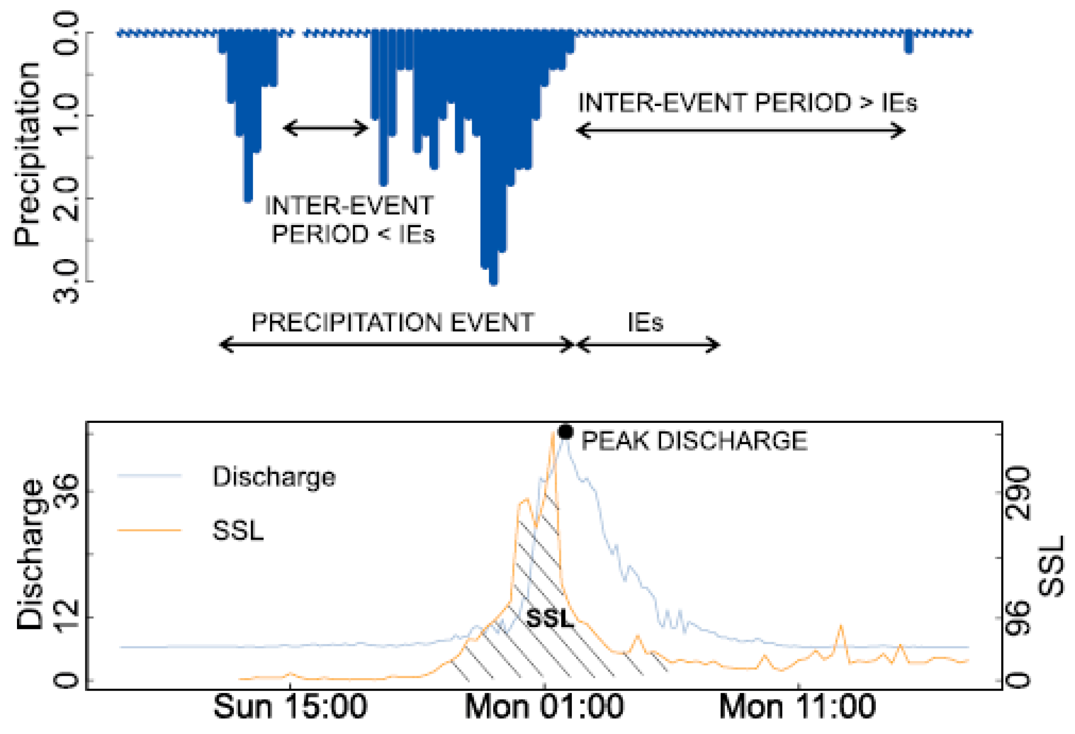
2.3. An Event-Based Sample Selection Methodology

In this study, a new approach using copula functions was proposed to estimate the SSL values based on the measured discharge and precipitation data. Figure 2 shows the methodology used for event definition and variables selection. The considered assumption was that the majority of sediment transport occurs only in the coincidence with the rainfall events. The first step was to separate continuous rainfall data into individual rainfall events. Two rainfall events were separated when the inter-event time (i.e., time without rainfall) between two consecutive rainfall events exceeded the selected inter-event (IEs) value. The start of the runoff and sediment transport event was selected as the time of the beginning of the rainfall event; the end of the runoff and sediment transport event was chosen at the IEs hours (days) after the end of the rainfall event (Figure 2). In case of small or even micro torrential basins, such as the Kuzlovec torrent, the time of concentration is usually very short, in most of such basins even shorter than 1 or 2 h (e.g., [47]). However, for larger basins such as the Mura River basin, much larger time of concentration values can be expected and, consequently, larger IEs values have to be selected (i.e., a few days) in order to capture also the recession part of the hydrograph and sedimentograph (i.e., to consider all transported material and hydrograph volume as a consequence of a rainfall event as part of one event). In both cases the IEs value was defined based on screening of the data, estimating the time of concentration, and assessing the longest duration of the falling limb of the hydrograph. Thus, the main idea was that the selected IEs value is slightly greater than the time of concentration and that the selected IEs value does not result in lumping of separate events into one event. For the Kuzlovec torrent where 20-min data was available this procedure was performed based on the screening of the data (e.g., time of concentration was estimated as the time period between end of the (effective) rainfall event and the end of the surface runoff or the end of the recession part of the hydrograph). However, for the larger and more complex Gornja Radgona station on the Mura River where only daily data was available the time of concentration was estimated with the help of isochrones that were determined based on the digital elevation model (DEM) of the catchment. The time between the start and the end point of the runoff and sediment transport event was defined as the duration of the event (Figure 2). The accumulated rainfall (P) was defined as a rainfall sum between the starting and ending point of the runoff and sediment transport event (Figure 2). The corresponding peak discharge variable (Q) was defined as the maximum discharge value during the runoff and sediment transport event (Figure 2). Furthermore, the corresponding suspended sediment load (SSL) was defined as the sum of the suspended sediment load rate (e.g., g/s) (Figure 2), which was transported during the runoff and sediment transport event (Figure 2). An event-based copula model, where consecutive events are assumed to be independent, was thus defined by using three variables: peak discharge (Q) (L/s or m³/s), accumulated rainfall (P) (mm), and suspended sediment load (SSL) (kg or t).

Before applying the copula model the autocorrelation in the marginal data was tested using the graphical acf test that is implemented in the software R [48]. Figure 3 shows the acf plot for both case studies (Kuzlovec torrent and Gornja Radgona station on the Mura River). In case of detected autocorrelation, different procedures such as computing differences between consecutive observations, applying filters or using other data transformations can be used to remove autocorrelation in the data (e.g., [49,50]). In our study the residuals of the Autoregressive–moving-average (ARMA) model were used for this purpose (e.g., [51]). Ljung-Box test was used for testing the null hypothesis of independence in a given time series, namely P, Q and SSL series for both case studies (Box.test function in program R [48] was used). This test was used to ensure that consecutive events are independent.

2.4. Copula Function

Copula function relates univariate marginal distribution functions with the joint multivariate probability distribution function. If X = (X₁, …, X_d) is a random vector, F its joint cumulative distribution function (CDF), and F₁, …, F_d, marginal CDFs, then by Sklar’s theorem [52] there exists a d-copula C:[0, 1]^d → [0, 1] such that:

$$\mathrm{F}\left(x_1,\dots ,x_d\right)=C\left(F_1\left(x_1\right),\dots ,F_d\left(x_d\right)\right).$$

(1)

If marginal cumulative distribution functions are all continuous, copula C is unique and U_i: = F(X_i) are uniformly distributed on [0, 1]. Moreover, if all CDFs are also strictly increasing, we obtain:

$$C\left(u_1,\dots ,u_d\right)=F\left(F_1^{-1}\left(u_1\right),\dots ,F_d^{-1}\left(u_d\right)\right).$$

(2)

On the other hand, for a given copula C and univariate CDFs F₁, …, F_d, Equation (1) defines a multivariate CDF F with marginals F₁, …, F_d.

Different copula functions were used in this study. For the Kuzlovec case where 21 events were available symmetric Archimedean copulas were selected. Clayton, Frank, Gumbel-Hougaard and Joe copula functions were chosen among a set of possible alternatives [53,54,55,56,57]. The trivariate symmetric Frank copula from the Archimedean family is defined with:

$$C_{\theta }\left(u_1,u_2,u_3\right)=-\frac{1}{\theta }\ln \left\{1+\frac{\left(\exp \left(-\theta u_1\right)-1\right)\left(\exp \left(-\theta u_2\right)-1\right)\left(\exp \left(-\theta u_3\right)-1\right)}{{\left(\exp \left(-\theta \right)-1\right)}^2}\right\},$$

(3)

where $\theta \in \left(-\infty ,\infty \right)\backslash \left\{0\right\}$ is a dependence parameter and $u_1,u_2,u_3\in \left[0,1\right]$. The corresponding bivariate copula is:

$$C_{\theta }\left(u_1,u_2\right)=-\frac{1}{\theta }\ln \left\{1+\frac{\left(\exp \left(-\theta u_1\right)-1\right)\left(\exp \left(-\theta u_2\right)-1\right)}{\left(\exp \left(-\theta \right)-1\right)}\right\}.$$

(4)

A possible alternative to the symmetric copula functions could be the asymmetric or fully nested copula functions from the Archimedean family (e.g., Clayton, Frank, Gumbel-Hougaard) (e.g., [32,53,54]). However, symmetric copulas can be used in cases when investigated variables are exchangeable. In order to assess the exchangeability the exchTest function that is implemented in program R copula package was used. More information about the selected test is given in the copula package reference manual. The asymmetric model can be alternative to the symmetric model in cases when the dependence between two variables is stronger than the dependence between the other two pairs (bivariate dependences within a multivariate frame are not the same). For more theoretical information about different copula functions that were used in this study and copula theory in general one should refer to [40,53,54,55,56,57,58].

In the case of the Gornja Radgona station in the Mura River the Khoudraji-Liebscher copula functions were used [59,60]. These copula functions were first introduced and discussed in hydrology by [30,61]. The cumulative distribution function for the three dimensional case is [59,60]:

$$C_{{\theta }_1,{\theta }_2}=C_1\left(u_1^{1-{\alpha }_1},u_2^{1-{\alpha }_2},u_3^{1-{\alpha }_3}\right)C_2\left(u_1^{{\alpha }_1},u_2^{{\alpha }_2},u_3^{{\alpha }_3}\right),$$

(5)

where $C_1\mathrm{and}{C}_2$ are two copula functions, $\mathrm{and}{\theta }_1\mathrm{and}{\theta }_2$ the parameters of these two copula functions (in case of trivariate symmetric Archimedean copulas). In our case independence copula [39,53,54,55] and trivariate symmetric Archimedean copulas (Clayton, Gumbel-Hougaard, Frank and Joe) were selected as possible candidates for the functions $C_1\mathrm{and}{C}_2$ (each of the Archimedean copula has one parameter). Further, α₁, α₂, α₃$\in \left[0,1\right]$are shape parameters [59,60]. The following combinations were tested in this study: (a) $C_1\mathrm{and}{C}_2$ are independence copulas (this model has 3 parameters: α₁, α₂, α₃); (b) $C_1\mathrm{and}{C}_2$ are independence copula and trivariate symmetric Archimedean copula (this model has 4 parameters: α₁, α₂, α₃ and${\theta }_1$); (c) $C_1\mathrm{and}{C}_2$ are trivariate symmetric Archimedean copulas (this model has 5 parameters: α₁, α₂, α₃ $\mathrm{and}{\theta }_1\mathrm{and}{\theta }_2$). This means that for case (a) 1 combination; (b) 8 combinations; (c) 16 combinations (all possible combinations of Clayton, Frank, Joe and Gumbel-Hougaard copulas were used) for the function in Equation (5) were tested.

The maximum pseudo-likelihood method was selected for the estimation of the copula parameters [62]. The adequacy of the selected copula functions was tested using the Cramér-von Mises test S_n, which was defined by [63]. The R copula package was used for copula parameter estimation and the goodness-of-fit test presented in this paper [64]. The most suitable copula function among Frank, Clayton, Joe, Gumbel-Hougaard and Khoudraji-Liebscher copula was selected using the model selection criterion (function xvCopula) that is based on the k-fold cross-validation and it is implemented in the program R copula package [64]. The detailed description of the criterion can be found in [65].

Various parametric and nonparametric distribution functions were selected as marginal CDFs, and marginal distribution parameters of the parametric distributions were estimated using the method of L-moments [66]. For the Kuzlovec case study where parametric distribution functions were used as marginal distribution functions the following distributions were selected: generalized extreme value (GEV), Gumbel, Pearson type 3, log-Pearson type 3, exponential, Generalized Pareto and normal [66]. More information about the selected parametric distribution can be found in [66]. In order to select the most suitable distribution the Akaike Information Criterion (AIC) was used. The adequacy of the selected distribution function was tested using the Cramér-von Mises test that is implemented in the program R lmomco package [67]. Additionally, the following nonparametric distribution function was used for the Gornja Radgona on the Mura River case study due to the larger number of analysed events [68,69]:

$$F_X\left(x\right)=\{\begin{array}{c}\frac{1}{n^{\prime }}\exp \left(\frac{x-X_{1:n}}{X_{2:n}-X_{1:n}}\right),x\le X_{1:n}\\ \left(1-ϵ\right)\frac{j}{n+1}+\epsilon \frac{k}{n+1},X_{j:n}<x<X_{k:n},j<k=1,\dots ,n^{\prime }\\ 1-\frac{1}{n^{\prime }}\exp \left(\frac{x-X_{n:n}}{X_{n:n}-X_{n-1:n}}\right),x\ge X_{n:n}\end{array}$$

(6)

where $n^{\prime }=n+1$, n is data sample length, $X_{i:n}$ ($i=1,\dots ,n$) is the generic order statistics (sample arranged in the ascending order), $X_{j:n}$ and $X_{k:n}$ are the order statistics closest to x and $ϵ=\left(x-X_{j:n}\right)/\left(X_{k:n}-X_{j:n}\right)$ [70]. More information about this nonparametric distribution function can be found [70,71].

In order to estimate the SSL values based on the Q and P values, the conditional CDF of U₃ (U₃ = F_SSL(SSL)) given the values of U₁ (U₁ = F_Q(Q)) and U₂ (U₂ = F_P(P)) can be shown to be (Appendix A):

$$C_{\theta }\left(u_3|u_1,u_2\right):=P(U_3\le u_3|U_1=u_1,U_2=u_2)=\frac{{\partial }^2{C}_{\theta }\left(u_1,u_2,u_3\right)}{\partial u_1\partial u_2}/\frac{{\partial }^2{C}_{\theta }\left(u_1,u_2\right)}{\partial u_1\partial u_2}$$

(7)

where $C_{\theta }\left(u_1,u_2,u_3\right)$ and $C_{\theta }\left(u_1,u_2\right)$ are given in Equations (3) and (4), respectively. Furthermore, Khoudraji-Liebscher copula function (e.g., Equation (5)) can be selected instead of the symmetric copula.

The procedure for estimating the SSL values given the known (measured) values Q and P was as follows:

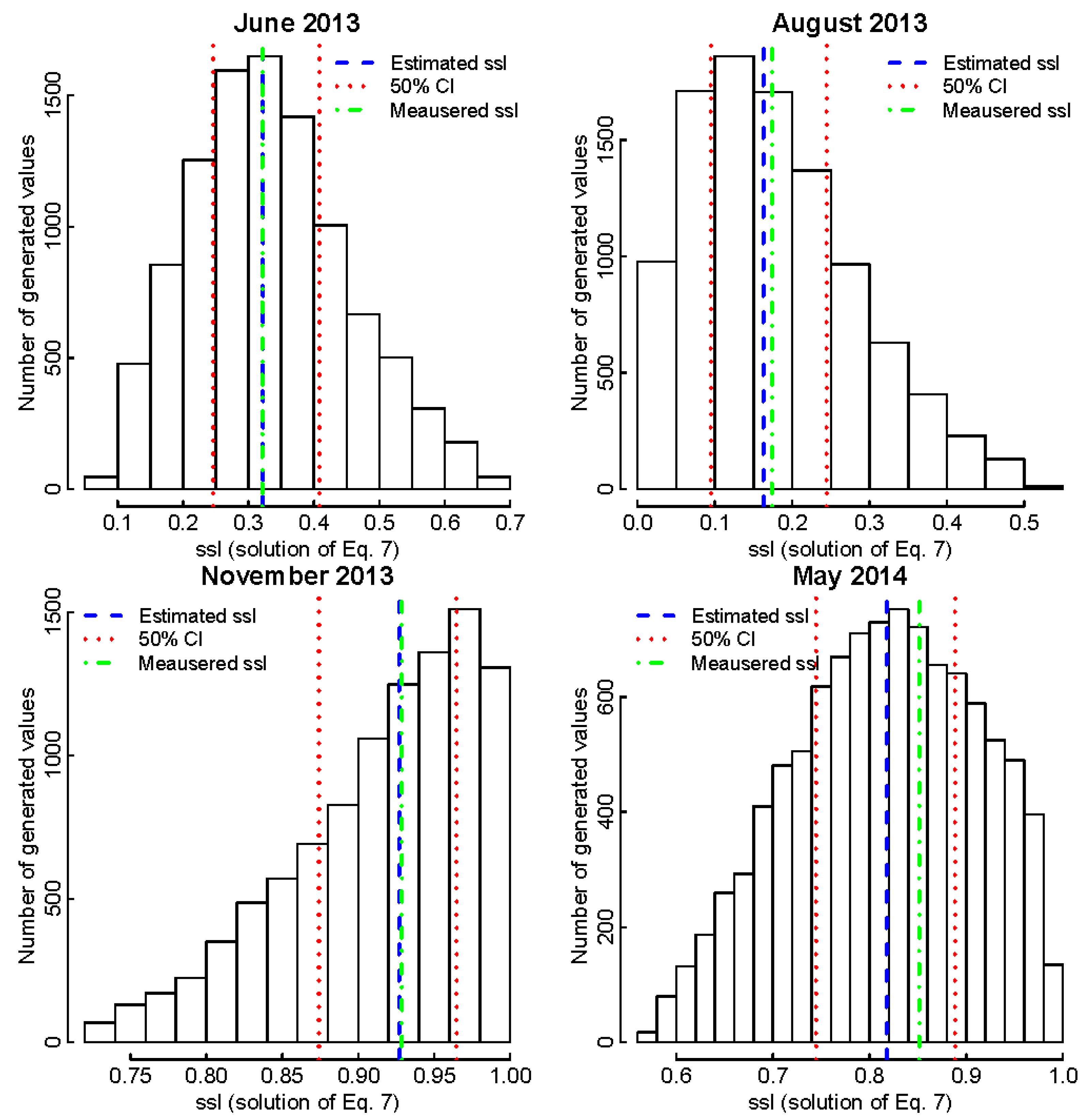
• For each measured (known) pair of variables Q and P 10,000 uniform random variables [0, 1] were generated;
• For each of the 10,000 uniform randomly generated variables, Equation (7) was solved numerically using the Newton’s method for solving nonlinear equations [72];
• For each of the solutions of Equation (7), the inverse Probability Integral Transform (PIT) ($SSL=F_{SSL}^{\left[-1\right]}\left(u_3\right)$) was used to transform the solution from the copula space [0, 1] to the real space and consequently estimate the SSL value.
• For each known pair of variables Q and P, which corresponds to the specific event, a sample of 10,000 possible SSL values was obtained.
• The median value of all 10,000 possible SSL values was selected as the estimated SSL value and 50% confidence intervals for each event were also determined. Alternatively, the mode could be selected as the most likely value in some other cases.

2.5. Regression Models and Performance Criteria

The performance of the proposed copula model was compared with the multiple regression (MLR) model and exponential model (EXP) that can be defined with the following equations:

$$SS{L}_{MLR}=a+b\times P+c\times Q$$

(8)

$$SS{L}_{EXP}=\exp \left(d\right)\times Q^e$$

(9)

where a, b, c, d and e are parameters that were estimated using the least-square method. Several performance criteria described by [69] such as Mean absolute error (MAE), Root mean square error (RMSE), Nash-Sutcliffe Efficiency (NSE) index and Coefficient of determination (R²) and residual analysis (graphical presentation and descriptive statistics of residuals) were used for comparison of different methods (Copula, MLR and EXP).

3. Results and Discussion

3.1. Kuzlovec Torrent

3.1.1. Estimation of Copula Model Parameters for the Kuzlovec Torrent

The methodology presented in Section 2 for the estimation of the SSL values based on the measured Q and P was tested using the high-frequency data measured in the Kuzlovec torrent. The IEs value of 6 h was selected for the Kuzlovec torrent. It was found that the IEs of 6 h is the reasonable selection for the considered torrent. Because the selected IEs value is greater than the time of concentration (usually less than 1 h) the consecutive events can be treated independently [73]. However, the selection of the IEs can have significant impact on the defined sample and consequently also on the results [74] because it influences both the total rainfall amounts (P) and the SSL values. This means that longer IEs values could result in larger P values due to lumping of consecutive events into one event. This would probably lead to larger SSL values but we argue that the impact on the Q values may be smaller. Thus, the dependence structure of the collected data sample may change (Figure 4). Moreover, larger IEs value would also lead to more multiple-peaks events. Altogether 21 complete events (Q, P, and SSL), which were defined using the procedure described in Section 2 (Figure 2) and that occurred in all four seasons from June 2013 to May 2014, were used for estimating the copula and marginal parametric CDFs parameters (Figure 4).

Table 2. Summary statistics of the defined variables for the data from the Kuzlovec torrent.

Statistic/Variable	P (mm)	Q (L/s)	SSL (kg)
Min	1.6	6.7	0.4
1st quartile	16.8	9.9	3.9
Median	23.0	15.6	17.2
Mean	27.2	31.1	94.3
3rd quartile	37.8	45.8	167.9
Max	63.0	125.9	470.3

shows the basic properties of the defined sample.

First the autocorrelation in the marginal data was tested. Figure 3 shows the acf plots for the three variables for the data from the Kuzlovec torrent. There was no significant autocorrelation in the data (Figure 3). This is confirmed by the Ljung-Box test results for the P, Q, and SSL series that were 1.8 (p-value: 0.18), 1.7 (p-value: 0.19) and 0.77 (p-value: 0.38), respectively. The next step of the copula approach was to assess the dependence between the pairs of considered variables (cor.test function was used [48]; null hypothesis: variables are independent; alternative hypothesis: variables are not independent). The Kendall’s correlation coefficients between pairs of variables Q-P, Q-SSL, and P-SSL were 0.70 (z-value: 4.4; p-value: 0.0001), 0.79 (z-value: 5.0; p-value: 6 × 10⁻⁷), and 0.70 (z-value: 4.4; p-value: 0.0001), respectively. Therefore, the null hypothesis was rejected with selected significance level of 0.05. The calculated correlation coefficients indicate that the dependence between pairs of variables is similar. Moreover, the exchangeability test results for pairs of variables P-Q, P-SSL and Q-SSL were 0.022 (p-value: 0.99), 0.022 (p-value: 0.98) and 0.021 (p-value: 0.72), respectively. This indicates that the selection of symmetric copula functions (e.g., Clayton, Frank, Gumbel-Hougaard, Joe), which have one parameter to model the dependence among three variables, seems reasonable for the Kuzlovec case study.

Before applying the copula function, marginal distribution functions were defined. Different distribution functions were tested and the most suitable were selected using the AIC criterion. For the P, Q and SSL the distribution functions with a minimum AIC value were Gumbel, Pearson type 3 and log-Pearson type 3, respectively. Aforementioned functions were also tested using the Cramér-von Mises test (lmomco package) and the results were 0.044 (p-value: 0.91), 0.082 (p-value: 0.69) and 0.135 (p-value: 0.44) for the P, Q and SSL, respectively. This indicates that selected distribution functions could not be rejected at the selected significance level (0.05). The marginal distribution parameters were estimated using the method of L-moments [67]. The location, scale, and shape parameters for the Pearson type 3 CDF (Q) were 31.1, 31.6, and 2.3, respectively. Likewise, the location and scale parameters for the Gumbel CDF (P) were 19.2 and 13.7, respectively. Furthermore, the location, scale, and shape parameters for the log-Pearson type 3 CDF were 3.0, 2.2, and −0.14, respectively. More information about the CDF and parameters can be found in [67]. The next step of the procedure was to estimate the copula parameter and to select the most suitable copula function. Clayton, Frank, Joe and Gumbel-Hougaard copula functions were compared using the leave-one-out cross-validation model selection criterion [65]. The criterion results were 24.4, 29.0, 25.0 and 16.1 for the Gumbel-Hougaard, Frank, Clayton and Joe copulas, respectively. According to these results the Frank copula should be selected (the largest value of the selected criterion). This function could not be rejected by the Cramér-von Mises test [63,64] at the selected significance level of 0.05 (statistics: 0.06; p-value: 0.26). Thus, this copula function was selected as the most suitable for the Kuzlovec torrent case study. The Frank copula parameter (Equation (3)) was estimated (Ɵ = 10.5) using the maximum pseudo-likelihood method [62]. Therefore, the Frank copula function was selected to define the model for estimating the SSL values using the data from the Kuzlovec torrent.

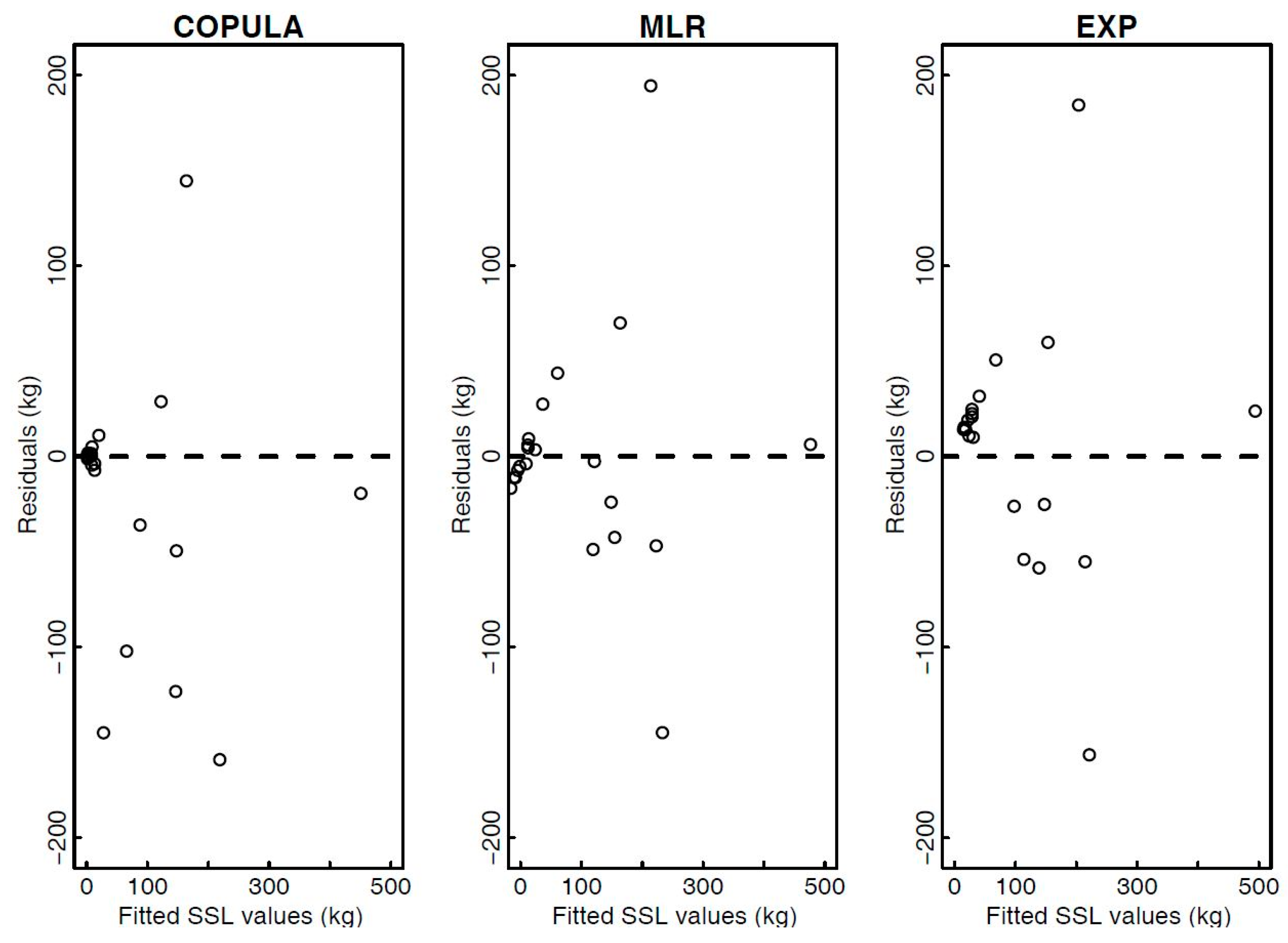
3.1.2. Comparison with Other SSL Estimation Techniques and Estimation of SSL Values Based on Measured Q and P

The procedure described in Section 2 was used to estimate the SSL values based on the measured Q and P. For each pair of measured variables (Q and P), which represents a potential event without SSL measurements, 10,000 possible SSL values were obtained. Figure 5 shows a distribution of Equation (7) solutions for four events, which occurred in different seasons. The median value of all 10,000 possible SSL values for one event was selected as the estimated SSL value, which was eventually transformed to real space using the inverse PIT. Furthermore, 50% confidence intervals (first and third quartile values were selected) for each event were also determined and are presented in Figure 5. Moreover, actual measured SSL values are also shown in Figure 5. It should be noted that November 2013 and May 2014 events were among the events with the highest SSL values. On the other hand, June 2013 and August 2013 events can be defined as low-medium magnitude events. The results indicate that the copula is able to reproduce both low-medium and medium-high magnitude sediment transport events.

In the next step of the study the proposed event-based copula methodology for estimating the SSL values was compared with some other possible estimation techniques (Equations (8) and (9)). Based on 21 events, which were also used in constructing the event-based copula model (Section 2), the MLR and EXP model were defined and tested to estimate the SSL values. The least-square method was used to estimate the MLR model parameters and the final constructed model was as follows $SSL=-42.92+0.61\times P+3.88\times Q$. Furthermore, the same method was applied to estimate the exponential model parameters, and the resulting model was: $SSL=\exp \left(0.42\right)\times Q^{1.20}$. In the next step, the copula, MLR, and EXP models were used to estimate the SSL values based on the measured Q and P variables. Figure 6 shows diagnostic plots for the three compared models, while some commonly used performance criteria are presented in

Table 3. Performance criteria results and summary statistics for the estimated SSL values for the Kuzlovec torren.

Statistic/Model	Copula	MLR	EXP
MAE (kg)	40.3	34.76	42.5
RMSE (kg)	68.3	59.42	61.7
NSE	0.74	0.80	0.79
R2	0.77	0.80	0.79
Min SSL (kg)	1	−16.1	14.7
Median SSL (kg)	13.3	36.47	40.6
Max SSL (kg)	451	476.5	494.0

. According to the different performance criteria [69], the proposed copula model yields the worst fit among the tested models. However, the diagnostic plots (Figure 6) demonstrate that the residuals are generally the smallest when using the copula model. The calculated residuals were approximately normally distributed and there was no autocorrelation in the residuals. The median residual values for three models were −1.2, −3.8, and 14.3 kg for the copula, MLR, and EXP model, respectively. The copula model is able to better reproduce the low-medium magnitude events, while the differences among compared methods in case of medium-high magnitude events are smaller and one could also argue that MLR and EXP models gave better fit to the data compared to the low-medium magnitude events. However, Figure 5 shows that the copula model can also be used to model medium-high magnitude events. Furthermore, a comparison was also made for the single-peak and multiple-peaks events (Figure 4). While for the single-peak events copula model yielded the smallest residual values, the differences among tested methods for the multiple-peaks events were smaller and the proposed copula model gave the worst results. However, one should keep in mind that only 4 events were defined as multiple-peaks and actually all these events were composed from 2 peaks. Moreover, the summary statistics for the estimated SSL values indicate that the copula model gives the most accurate estimates of the measured SSL values (comparison of Table 2 and Table 3). Using the MLR model the estimated SSL values for some smaller rainfall events (e.g., P < 10 mm) were estimated as negative (Table 3), which is not a meaningful result. Moreover, the EXP model generally overestimated these smaller magnitude events (Table 2 and Table 3).

The fit between the measured and estimated data could be improved with the inclusion of additional information in the model. For example, bed load data, antecedent soil moisture conditions and antecedent sediment transport data are just some of the possible options in case that this information is available. For the Kuzlovec torrent the relationship between the 1-day (ANTP1), 3-day (ANTP3) and 5-day (ANTP5) antecedent rainfall and SSL was also evaluated. The Kendall correlation coefficients for ANTP1-SSL, ANTP3-SSL and ANTP5-SSL were 0.17 (p-value: 0.28), −0.08 (p-value: 0.61) and 0.02 (p-value: 0.89), respectively, which indicates that antecedent rainfall is not a good predictor of the SSL for the Kuzlovec torrent. One of the possible alternatives to improve the copula model results can also be use of copula function with more parameters (e.g., Khoudraji-Liebscher copula) but one should keep in mind that over-parametrization could occur in such case, especially estimates of fitted parameters can be uncertain in case of 21 events. Moreover, nonparametric distribution function could be an alternative to the parametric distribution in order to reduce the number of parameters. In the case of the Kuzlovec torrent extreme flash flood occurred in August 2014 that caused intense sediment transport and changes in the location of the torrent channel thalweg [75]. This means that additional measurements should be performed at this location in order to confirm that the proposed model (either copula or regression model) is still valid for this location after this extreme event with more than 100 years return period according to the rainfall data analysis [75].

Due to the smallest residual values and because probabilistic estimation of the SSL values can be obtained with the copula model this method was chosen to estimate the SSL values for the events when SSC observations were not performed. Based on the methodology presented in Section 2 the SSL estimates were conducted for 92 events which occurred in all four seasons. Months June, July, and August were classified as summer, September, October, and November as autumn, December, January, and February as winter and March, April, and May as spring. For events where accumulated rainfall (P) did not exceed 1 mm the estimates of SSL were not performed and further results are not presented.

Table 4. Basic properties of the SSL, Q and P values for different seasons for the Kuzlovec torrent.

Season	Mean P (mm)	Max Q (L/s)	SSL (kg)	SSL0.25 (kg)	SSL0.75 (kg)
Summer 2013	11.4	36.0	99	58	172
Autumn 2013	17.8	125.9	1429	805	2787
Winter 2013–2014	26.8	138.6	1724	989	3293
Spring 2014	12.1	43.5	360	217	645

shows the results of the estimation procedure for different seasons. The results demonstrate that approximately 3.6 t of SSL were transported through the measuring cross section in the Kuzlovec torrent in the observed period (June 2013–May 2014) (Table 4). The lower confidence interval was 2.1 t and the upper one 6.9 t (Table 4). One can notice that most of the SSL was transported during winter 2013/2014 (Table 4), which was relatively warm and with small amounts of snow in the considered period. The highest P and Q values are also characteristics of the winter period. The autumn 2013 contributed about 40% of the total SSL, while in summer 2013 and spring 2014 together about 12% of SSL was transported. A more comprehensive seasonality analysis could be done if more than one year of data would be available. However, one should also keep in mind that from June 2013 to May 2014 a total of 1613 mm of rainfall was measured in the investigated basin, which is below the long-term average for the analyzed area (about 1700 mm). Furthermore, none of the rainfall events was really extreme. The maximum measured accumulated rainfall amount for one event was 89 mm, which occurred in January, and the duration of the event was about 2 days. This suggests that under different, more extreme, hydro-meteorological conditions significantly more material could be transported even in the small torrential basin like Kuzlovec (up to ~5 or even 10 t/ha/year), because generally most of the material is transported during extreme events such as floods (e.g., [1,75]). One should keep in mind that for the Kuzlovec case study only 21 events were used for parameter estimation and fitting of the trivariate copula functions. This means that several types of uncertainties can affect estimation results due to the relatively small sample size: (i) model identifiability; (ii) estimates of the fitted parameters and (iii) ultimate estimates of the derived risks. However, the main aim of the study was to demonstrate that the proposed event-based copula model can be used for estimating SSL values based on the known Q and P values. Thus, the proposed methodology was additionally tested on another case study (Gornja Radgona station on the Mura River) where 281 events were available to fit the proposed copula model and to make an estimation of the SSL values using the copula model.

3.2. Gornja Radgona Station on the Mura River

3.2.1. Estimation of Copula Model Parameters for the Gornja Radgona Station

The proposed copula model was also applied to the data from the Gornja Radgona station on the Mura River (Figure 1). The daily discharge, suspended sediment concentration, and precipitation (Cankova station) data from 1977 to 2005 were used. The same methodology as that for the Kuzlovec torrent was used for the event definition (Figure 2). However, the IEs value of 3 days was selected in order to separate individual events. Given that only daily data was available, the time of concentration was estimated using the Geographic information system (GIS) algorithm for the calculation of isochrones that uses DEM to estimate the isochrones [76]. The estimated time of concentration was about 64 h; therefore the IEs value of 3 days was selected for event separation. It was found that this value is sufficient to capture the recession part of hydrograph and sedimentograph. In the next step P, Q, and SSL variables were calculated for each event. A threshold of 30 mm (P) was applied to remove small magnitude events. At the end 281 events were used to construct the copula-based model (Figure 7).

Table 5. Summary statistics of the defined variables for the data from the Gornja Radgona station on the Mura River.

Statistic/Variable	P (mm)	Q (m3/s)	SSL (t)
Min	30.1	62.7	357.7
1st quartile	37.7	169	3453
Median	49.3	244.3	9317
Mean	58.3	295.1	26,410
3rd quartile	68.4	374	26,500
Max	186.9	1237	303,000

shows the summary statistics of the defined variables. One of the important aspects in the SSL estimation is also that the relationship between the discharge and sediment transport did not significantly change in the observed period (e.g., impact of extreme flood). For the Gornja Radgona station on the Mura River this can be confirmed with the SSC trend test for the period from 1977 to 2005 [4]. The results indicate that SSC trend is not statistically significant [4]. This means that use of the complete data period (1977–2005) as one part seems reasonable. In case of statistically significant trend data sample should be divided into more parts depending on the data complexity and trend characteristics.

The acf plot was used to test autocorrelation in the marginal data. Moreover, the Ljung-Box test results were 1.9 (p-value: 0.17), 6.2 (p-value: 0.01) and 2.6 (p-value: 0.10) for the P, Q and SSL data, respectively. It was found that for Q data autocorrelation was significant (selected significance level 0.05). Therefore, the residuals of the ARMA model were used to remove the autocorrelation in the Q data. Figure 3 shows the acf plots for P, transformed Q, and SSL values with 0.95 confidence limits for the Gornja Radgona station on the Mura River. The next steps of the analyses were performed using the transformed data (residuals of the ARMA model). The Ljung-Box test result for the transformed Q data was 0.01 (p-value: 0.91).

The calculated Kendall correlation coefficients between pairs of variables Q-P, Q-SSL, and P-SSL were 0.29 (z-value: 7.3; p-value: 2 × 10⁻¹³), 0.64 (z-value: 15.9; p-value: 2 × 10⁻¹⁶) and 0.28 (z-value: 6.9; p-value: 4 × 10⁻¹²), respectively. These correlation coefficients do not depend on the transformation of the data. Moreover, the exchangeability test results for pairs of variables Q-P, Q-SSL, and P-SSL were 0.04 (p-value: 0.24), 0.01 (p-value: 0.94) and 0.04 (p-value: 0.15), respectively. Since the dependence between pairs of variables is not the same, the symmetric copula function with one parameter is not the most suitable model. Therefore, the Khoudraji-Liebscher copula function (Equation (5)) was used to model the data from the Gornja Radgona station on the Mura River. Different combinations of the Khoudraji-Liebscher copula were tested (independence copula and Joe, Clayton, Frank and Gumbel-Houaard copulas were used as C₁ and C₂ in Equation (5)). The adequacy of different combinations ((a), (b) and (c) defined in Section 2.4) was tested using the Cramér-von Mises test S_n. Based on the selected significance level of 0.05 the following combinations of C₁ and C₂ (Equation (5)) could not be rejected: (i) Joe-C₁ and Joe-C₂ (statistic: 0.10; p-value: 0.07); (ii) Gumbel-Hougaard-C₁ and Gumbel-Hougaard-C₂ (statistic: 0.08; p-value: 0.10) and (iii) Gumbel-Hougaard-C₁ and Joe-C₂ (statistic: 0.07; p-value: 0.14). In total 25 combinations were tested and all other combinations were rejected at the selected significance level of 0.05 ((a), (b) and (c) defined in Section 2.4). Moreover, to select the most suitable copula function the copula leave-one-out cross-validation selection criterion was used [65]. The criterion results were 162.1, 164.8 and 157 for the combinations (i), (ii) and (iii), respectively. Based on these results the combination of Gumbel-Hougaard-C₁ and Gumbel-Hougaard-C₂ was used for the estimation of the SSL values for the Gornja Radgona station. The selected model has 5 parameters. In some other cases different combination of C₁ and C₂ could be selected in order to reduce the number of parameters (over-parametrization issue). For example, the application of independence copula (case (a) defined in Section 2.4) leads to a model with 3 parameters, which is positive from the over-parametrization perspective. However, in this case study models with smaller number of parameters (cases (a) and (b) defined in Section 2.4) were rejected by the selected goodness-of-fit test for copula functions. The copula parameters were estimated using the maximum pseudo-likelihood method. The estimated parameters ${\theta }_1\mathrm{and}{\theta }_2$ for the Gumbel-Hougaard (C₁) and Gumbel-Hougaard (C₂) copulas were 1.78 and 3.12, respectively (where U₁ = F_Q(Q), U₂ = F_SSL (SSL) and U₃ = F_P(P) according to the notations used in Equation (5)). Moreover, the shape parameters α₁, α₂ and α₃ were 0.60, 0.63 and 2 × 10⁻⁵, respectively. Different parametric distributions such as Gumbel, Generalized Pareto, Pearson type 3, log-Pearson type 3 and GEV were tested but none of them gave an adequate fit to the data. Therefore, the nonparametric distribution function, which is defined with Equation (6), was used to model the selected variables (Q, P, and SSL). This distribution function was tested using the Kolmogorov-Smirnov test and for all variables the nonparametric distribution could not be rejected at the chosen significance level of 0.05.

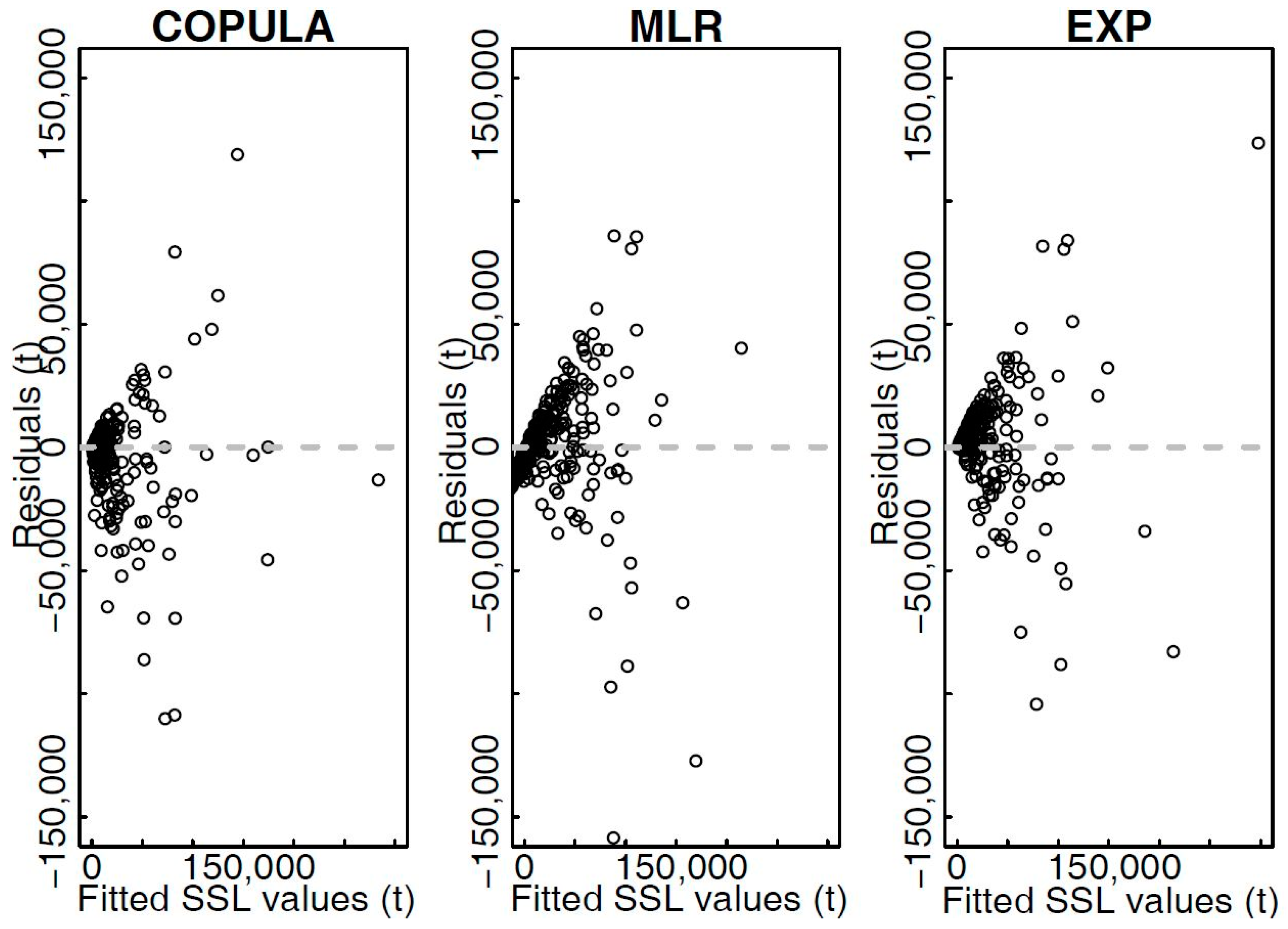
3.2.2. Comparison with Other SSL Estimation Techniques

In the next step, the SSL values were estimated using the copula, MLR, and EXP models. The MLR and EXP models were fitted to the original data.

Table 6. Performance criteria results and summary statistics for the estimated SSL values for the Gornja Radgona station on the Mura River.

Statistic/Model	Copula	MLR	EXP
MAE (t)	12,403	15,500	13,637
RMSE (t)	26,261	26,230	25,400
NSE	0.65	0.65	0.67
R2	0.66	0.65	0.67
Min SSL (t)	900	−20,020	1410
Median SSL (t)	8768	16,280	16,210
Max SSL (t)	283,500	214,500	297,900

shows the results for some commonly used performance criteria (e.g., [69]) and the summary statistics for the estimated SSL values using the copula model. For MLR and EXP models original data (autocorrelation in the Q data was not removed) was used. The copula parameters were estimated using the maximum pseudo-likelihood method which is based on ranks and selected nonparametric distributions are able to produce good fit to the marginal data independently of the transformation (residuals of the ARMA model). MLR and EXP models forms were $SSL=-33,349+31\times P+196\times Q$ and $SSL=\exp \left(-0.18\right)\times Q^{1.79}$, respectively. Figure 8 shows the diagnostic plots for the three compared models (original data was used for the MLR and EXP models). The copula and EXP models yield comparable results according to the selected performance criteria (Table 6). However, according to the residuals shown in Figure 8 the copula model gives a better fit to the measured data than the EXP model. This can also be confirmed with the median residual values for the copula, MLR, and EXP models, which were −195, 240, and 3918 t, respectively. Similar as for the Kuzlovec torrent, the copula model performs better in case of low-medium magnitude events while in case of medium-high magnitude events differences among tested methods are smaller. Since the daily data was only available not much can be said about the single-peak and multiple-peaks events in case of the Gornja Radgona station on the Mura River. Furthermore, the comparison of the summary statistics for the estimated and measured SSL values (Table 5 and Table 6) indicates that the proposed copula model can reproduce the actual SSL values better than the other two tested methods. Similarly as for the Kuzlovec torrent the MLR method yields negative SSL values for some specific low magnitude events. The Mura River catchment is larger and more complex than the Kuzlovec torrent and it is clear that the SSL estimation results are slightly better for the first case than for the latter one. However, these better results can be attributed to the larger number of events available to fit the model (reduced uncertainty in the parameter estimation), nonparametric distribution functions used and application of the Khoudraji-Liebscher copulas that are more suitable for complex dependence structure than symmetric copulas. We argue that similar performance of copula model can be expected in case of small and medium-large size catchments in case of similar sample sizes. Moreover, similar conclusion can also be made for the data frequency since comparable results are obtained using daily and 20-min data. However, prediction results can be improved with the inclusion of additional parameters in the model (e.g., antecedent conditions).

4. Conclusions

This paper presents a development and an application of the event-based copula model for estimating the SSL values based on the measured discharge and precipitation data. The high-frequency discharge, precipitation, and suspended sediment concentration measurements from a small experimental basin in Slovenia was used to set up the copula model (21 events that occurred from June 2013 to May 2014 were used). Furthermore, the copula model was additionally tested using the 29-years data series on daily discharge, suspended sediment concentration, and precipitation from the Gornja Radgona station on the Mura River where in total 281 events were used. In both case studies events occurred in different seasons. The main conclusions of this study are as follows:

• The proposed copula model for estimating the SSL values based on the measured Q and P values yielded meaningful results. According to some performance criteria and graphical presentation of the results the copula model gives comparable results to those obtained using other tested models (MLR and EXP). For the Gornja Radgona station the copula model yielded better fit to the actual measured SSL values than other tested methods. In this case study 281 events were available to estimate the copula model parameters and nonparametric distributions were selected as marginal distributions. However, for the Kuzlovec torrent much smaller number of events was analyzed and parametric distribution functions were used. The differences in the estimation results could also be a consequence of different copulas that were selected (symmetric and Khoudraji-Liebscher copulas). Using the copula model the probabilistic estimation of the SSL values can be obtained, which is not possible using other tested methods. Moreover, the smallest residual values were characteristic of the estimation procedure that was carried out using copula function, which indicates an important advantage of the proposed copula method compared to other tested methods. However, there were some differences between the low-medium and medium-high magnitude SSL events.
• The proposed copula based model is flexible. Both symmetric and Khoudraji-Liebscher copula functions were used to construct the copula model based on the dependence characteristics of the analyzed variables. Furthermore, other copula functions with more parameters and different properties such as Gaussian copula or Vine copulas could be used in this model to estimate the SSL values based on the Q and P. Similarly, also different marginal distribution functions can be selected, even nonparametric. The proposed copula model where nonparametric marginal distribution functions were used is more robust tool that is not significantly affected by transformations of the marginal data.
• An event-based copula model used in this study could easily be upgraded with additional variables (e.g., bedload, water electrical conductivity measurements, antecedent sediment transport conditions or antecedent soil moisture), because copula functions of higher dimensions can be constructed relatively easily. Moreover, similar model could also be used for the estimation of different environmental variables (e.g., biogeochemical model-water chemistry).
• Unlike some other techniques, the presented event-based model also captures the sediment lag effect. In the future it would be reasonable to consider also the sediment depletion (exhaustion) effect (e.g., antecedent sediment transport), which can have a considerable impact on the SSL values during consecutive events.
• The proposed event-based copula model can be a useful tool for estimating sediment budgets. The methodology was successfully applied to two different case studies, a small forested torrent and a larger river catchment and comparable results were obtained in both cases (in first case 20-min data was used while in the second case daily data was used).

The presented methodology for estimating SSL values should be additionally tested on the high-frequency data from other parts of the world, while SSL estimation results could be compared using additional estimation techniques (e.g., those that can be used for estimating SSC time-series). However, the results of this study, using the one-year high-frequency experimental data from the Kuzlovec torrent (21 events) and the 29 years of daily data from the Gornja Radgona station on the Mura River in Slovenia (281 events), demonstrate that the proposed methodology has a promising potential as it has already yielded meaningful results for the two selected field case studies.

References

1. Lenzi, M.A.; Mao, L.; Comiti, F. Interannual variation of suspended sediment load and sediment yield in an alpine catchment. Hydrol. Sci. J. 2003, 48, 899–915. [Google Scholar] [CrossRef]
2. Tena, A.; Batalla, R.J.; Vericat, D.; Lopez-Tarazon, J.A. Suspended sediment dynamics in a large regulated river over a 10-year period (the lower Ebro, NE Iberian Peninsula). Geomorphology 2011, 125, 73–84. [Google Scholar] [CrossRef]
3. Gorgoglione, A.; Gioia, A.; Iacobellis, V.; Ferruccio Piccinni, A.; Ranieri, E. A Rationale for Pollutograph Evaluation in Ungauged Areas, Using Daily Rainfall Patterns: Case Studies of the Apulian Region in Southern Italy. Appl. Environ. Soil Sci. 2016. [Google Scholar] [CrossRef]
4. Bezak, N.; Šraj, M.; Mikoš, M. Analyses of suspended sediment loads in Slovenian rivers. Hydrol. Sci. J. 2016, 61, 1094–1108. [Google Scholar] [CrossRef]
5. Ulaga, F. Monitoring suspendiranega materiala v slovenskih rekah monitoring of suspended matter in Slovenian rivers. Acta Hydrotech. 2005, 23, 117–127. (In Slovene) [Google Scholar]
6. Gray, J.R.; Gartner, J.W. Technological advances in suspended-sediment surrogate monitoring. Water Resour. Res. 2009, 45, 20. [Google Scholar] [CrossRef]
7. Wren, D.G.; Barkdoll, B.D.; Kuhnle, R.A.; Derrow, R.W. Field techniques for suspended-sediment measurement. J. Hydraul. Eng. 2000, 126, 97–104. [Google Scholar] [CrossRef]
8. Lenzi, M.A.; D’Agostino, V.; Billi, P. Bedload transport in the instrumented catchment of the Rio Cordon Part I: Analysis of bedload records, conditions and threshold of bedload entrainment. Catena 1999, 36, 171–190. [Google Scholar] [CrossRef]
9. Lenzi, M.A.; Marchi, L. Suspended sediment load during floods in a small stream of the Dolomites (northeastern Italy). Catena 2000, 39, 267–282. [Google Scholar] [CrossRef]
10. Rickenmann, D. Sediment transport in Swiss torrents. Earth Surf. Process. Landf. 1997, 22, 937–951. [Google Scholar] [CrossRef]
11. Soler, M.; Latron, J.; Gallart, F. Relationships between suspended sediment concentrations and discharge in two small research basins in a mountainous Mediterranean area (Vallcebre, Eastern Pyrenees). Geomorphology 2008, 98, 143–152. [Google Scholar] [CrossRef]
12. Habersack, H.M.; Laronne, J.B. Bed load texture in an alpine gravel bed river. Water Resour. Res. 2001, 37, 3359–3370. [Google Scholar] [CrossRef]
13. Bonacci, O.; Oskorus, D. The changes in the lower Drava River water level, discharge and suspended sediment regime. Environ. Earth Sci. 2010, 59, 1661–1670. [Google Scholar] [CrossRef]
14. Harrington, S.T.; Harrington, J.R. An assessment of the suspended sediment rating curve approach for load estimation on the Rivers Bandon and Owenabue, Ireland. Geomorphology 2013, 185, 27–38. [Google Scholar] [CrossRef]
15. Horowitz, A. An evaluation of sediment rating curves for estimating suspended sediment concentrations for subsequent flux calculations. Hydrol. Process. 2003, 17, 3387–3409. [Google Scholar] [CrossRef]
16. Horowitz, A. Determining annual suspended sediment and sediment-associated trace element and nutrient fluxes. Sci. Total Environ. 2008, 400, 315–343. [Google Scholar] [CrossRef] [PubMed]
17. Araujo, H.A.; Cooper, A.B.; Hassan, M.A.; Venditti, J. Estimating suspended sediment concentrations in areas with limited hydrological data using a mixed-effects model. Hydrol. Process. 2012, 26, 3678–3688. [Google Scholar] [CrossRef]
18. Khanchoul, K.; El Abidine Boukhrissa, Z.; Acidi, A.; Altschul, R. Estimation of suspended sediment transport in the Kebir drainage basin, Algeria. Quat. Int. 2012, 262, 25–31. [Google Scholar] [CrossRef]
19. Holtschlag, D.J. Optimal estimation of suspended-sediment concentrations in streams. Hydrol. Process. 2001, 15, 1133–1155. [Google Scholar] [CrossRef]
20. Moliere, D.R.; Evans, K.G.; Saynor, M.J.; Erskine, W.D. Estimation of suspended sediment loads in a seasonal stream in the wet-dry tropics, Northern Territory, Australia. Hydrol. Process. 2004, 18, 531–544. [Google Scholar] [CrossRef]
21. Nourani, V. Using artificial neural networks (ANNs) for sediment load forecasting of Talkherood River mouth. J. Urban Environ. Eng. 2009, 3, 1–6. [Google Scholar] [CrossRef]
22. Rajaee, R.; Mirbagheri, S.A.; Zounemar-Kermani, M.; Nourani, V. Daily suspended sediment concentration simulation using ANN and neuro-fuzzy models. Sci. Total Environ. 2009, 12, 4916–4927. [Google Scholar] [CrossRef] [PubMed]
23. Senthil Kumar, A.R.; Ojha, C.S.P.; Goyal, M.K.; Singh, R.D.; Swamee, P.K. Modeling of Suspended Sediment Concentration at Kasol in India Using ANN, Fuzzy Logic, and Decision Tree Algorithms. J. Hydrol. Eng. 2012, 17, 394–404. [Google Scholar] [CrossRef]
24. Lafdani, E.K.; Nia, A.M.; Ahmadi, A. Daily suspended sediment load prediction using artificial neural networks and support vector machines. J. Hydrol. 2013, 478, 50–62. [Google Scholar] [CrossRef]
25. McBean, E.A.; Al-Nassri, S. Uncertainty in Suspended Sediment Transport Curves. J. Hydrol. Eng. 1988, 114, 63–74. [Google Scholar] [CrossRef]
26. Isik, S. Regional rating curve models of suspended sediment transport for Turkey. Earth Sci. Inform. 2013, 6, 87–98. [Google Scholar] [CrossRef]
27. Tramblay, Y.; Ouarda, T.B.M.J.; St-Hilaire, A.; Poulin, J. Regional estimation of extreme suspended sediment concentrations using watershed characteristics. J. Hydrol. 2010, 380, 305–317. [Google Scholar] [CrossRef]
28. Roman, D.C.; Vogel, R.M.; Schwarz, G.E. Regional regression models of watershed suspended-sediment discharge for the eastern United States. J. Hydrol. 2012, 472–473, 53–62. [Google Scholar] [CrossRef]
29. Grimaldi, S.; Serinaldi, F. Asymmetric copula in multivariate flood frequency analysis. Adv. Water Resour. 2006, 29, 1155–1167. [Google Scholar] [CrossRef]
30. Durante, F.; Salvadori, G. On the construction of multivariate extreme value models via copulas. Environmetrics 2010, 21, 143–161. [Google Scholar] [CrossRef]
31. Chebana, F.; Ouarda, T.B.M.J. Multivariate quantiles in hydrological frequency analysis. Environmetrics 2011, 22, 63–78. [Google Scholar] [CrossRef]
32. Bezak, N.; Mikoš, M.; Šraj, M. Trivariate Frequency Analyses of Peak Discharge, Hydrograph Volume and Suspended Sediment Concentration Data Using Copulas. Water Resour. Manag. 2014, 28, 2195–2212. [Google Scholar] [CrossRef]
33. Šraj, M.; Bezak, N.; Brilly, M. Bivariate flood frequency analysis using the copula function: A case study of the Litija station on the Sava River. Hydrol. Process. 2015, 29, 225–238. [Google Scholar] [CrossRef]
34. Grimaldi, S.; Serinaldi, F. Design hyetograph analysis with 3-copula function. Hydrol. Sci. J. 2006, 51, 223–238. [Google Scholar] [CrossRef]
35. Singh, V.P.; Zhang, L. IDF curves using the Frank Archimedean copula. J. Hydrol. Eng. 2007, 12, 651–662. [Google Scholar] [CrossRef]
36. Bardossy, A.; Li, J. Geostatistical interpolation using copulas. Water Resour. Res. 2008, 44. [Google Scholar] [CrossRef]
37. Corbella, S.; Stretch, D.D. Simulating a multivariate sea storm using Archimedean copulas. Coast. Eng. 2013, 76, 68–78. [Google Scholar] [CrossRef]
38. Salvadori, G.; De Michele, C. Frequency analysis via copulas: Theoretical aspects and applications to hydrological events. Water Resour. Res. 2004, 40. [Google Scholar] [CrossRef]
39. Salvadori, G.; De Michele, C.; Kottegoda, N.T.; Rosso, R. Extremes in Nature: An Approach Using Copulas; Springer: Dordrecht, The Netherlands, 2007. [Google Scholar]
40. Wong, G.; Lambert, M.F.; Leonard, M.; Metcalfe, A.V. Drought Analysis Using Trivariate Copulas Conditional on Climatic States. J. Hydrol. Eng. 2010, 15, 129–141. [Google Scholar] [CrossRef]
41. Callau Poduje, A.C.; Belli, A.; Haberlandt, U. A Dam risk assessment based on univariate versus bivariate statistical approaches: A case study for Argentina. Hydrol. Sci. J. 2014, 59, 2216–2232. [Google Scholar] [CrossRef]
42. STAHY. Available online: http://www.stahy.org/Activities/STAHYReferences/ReferencesonCopulaFunctiontopic/tabid/78/Default.aspx (accessed on 15 July 2017).
43. Shiau, J.T.; Chen, T.J. Quantile Regression-Based Probabilistic Estimation Scheme for Daily and Annual Suspended Sediment Loads. Water Resour. Manag. 2015, 29, 2805–2818. [Google Scholar] [CrossRef]
44. Šraj, M.; Rusjan, S.; Petan, S.; Vidmar, A.; Mikoš, M.; Globevnik, L.; Brilly, M. The experimental watersheds in Slovenia. IOP Conf. Ser. 2008, 4, 1–13. [Google Scholar] [CrossRef]
45. Agencija Republike Slovenije za Okolje (ARSO). Available online: http://www.arso.gov.si/ (accessed on 10 January 2017).
46. Bezak, N.; Šraj, M.; Rusjan, S.; Kogoj, M.; Vidmar, A.; Sečnik, M.; Brilly, M.; Mikoš, M. Comparison between two adjacent experimental torrential watersheds: Kuzlovec and Mačkov graben. Acta Hydrotech. 2013, 26, 85–97. (In Slovene) [Google Scholar]
47. American Institute of Hydrology. Coastal Hydrology and Processes: Proceedings of the AIH 25th Anniversary Meeting & International Conference “Challenges in Coastal Hydrology and Water Quality”; Singh, V.P., Xu, Y.J., Eds.; Water Resources Publications: Highland Ranch, CO, USA, 2006; 509p. [Google Scholar]
48. R Development Core Team. R: A Language and Environment for Statistical Computing; R Foundation for Statistical Computing: Vienna, Austria, 2015. [Google Scholar]
49. Miao, C.; Ni, J. Implement of filter to remove the autocorrelation’s influence on the Mann-Kendall test: A case in hydrological series. J. Food Agric. Environ. 2010, 8, 1241–1246. [Google Scholar]
50. Hyndman, R.J.; Athanasopoulos, G. Forecasting: Principles and Practice; Otexts: Melbourne, Australia, 2013. [Google Scholar]
51. Hipel, K.W.; McLeod, A.T. Time Series Modelling of Water Resources and Environmental Systems; Elsevier Science: Amsterdam, The Netherlands, 1994. [Google Scholar]
52. Sklar, A. Fonction de répartition à n dimensions et leurs marges. Publications de L’Institute de Statistique 1959, 8, 229–231. [Google Scholar]
53. Joe, H. Multivariate Models and Dependence Concepts; Chapman & Hall: London, UK; New York, NY, USA, 1997. [Google Scholar]
54. Nelsen, R.B. An Introduction to Copulas; Springer: New York, NY, USA, 2006. [Google Scholar]
55. Durante, F.; Sempi, C. Principles of Copula Theory; CRC/Chapman & Hall: Boca Raton, FL, USA, 2015. [Google Scholar]
56. Genest, C.; Favre, A. Everything You Always Wanted to Know about Copula Modeling but Were Afraid to Ask. J. Hydrol. Eng. 2007, 12, 347–368. [Google Scholar] [CrossRef]
57. Salvadori, G.; Durante, F.; Tomasicchio, G.R.; D’Alessandro, F. Practical guidelines for the multivariate assessment of the structural risk in coastal and off-shore engineering. Coast. Eng. 2015, 95, 77–83. [Google Scholar] [CrossRef]
58. Pappada, R.; Durante, F.; Salvadori, G. Quantification of the environmental structural risk with spoiling ties: Is randomization worthwhile? Stoch. Environ. Res. Risk Assess. 2016. [Google Scholar] [CrossRef]
59. Khoudraji, A. Contributions à L’étude des Copules et àla Modélisation des Valeurs Extremes Bivariées. Ph.D. Thesis, Université Laval, Quebec City, QC, Canada, 1995. [Google Scholar]
60. Liebscher, E. Construction of asymmetric multivariate copulas. J. Multivar. Anal. 2008, 99, 2234–2250. [Google Scholar] [CrossRef]
61. Salvadori, G.; De Michele, C. Multivariate multiparameter extreme value models and return periods: A copula approach. Water Resour. Res. 2010, 46. [Google Scholar] [CrossRef]
62. Genest, C.; Ghoudi, K.; Rivest, L.P. A semiparametric estimation procedure of dependence parameters in multivariate families of distributions. Biometrika 1995, 82, 543–552. [Google Scholar] [CrossRef]
63. Genest, C.; Remillard, B.; Beaudoin, D. Goodness-of-fit tests for copulas: A review and a power study. Insur. Math. Econ. 2009, 44, 199–213. [Google Scholar] [CrossRef]
64. Kojadinovic, I.; Yan, J. Modeling Multivariate Distributions with Continuous Margins Using the copula R Package. J. Stat. Softw. 2010, 34. [Google Scholar] [CrossRef]
65. Grønneberg, S.; Hjort, N.L. The copula information criteria. Scand. J. Stat. 2014, 41, 436–459. [Google Scholar] [CrossRef] [Green Version]
66. Hosking, J.R.M.; Wallis, J.R. Regional Frequency Analysis: An Approach Based on L-Moments; Cambridge University Press: Cambridge, UK, 1997. [Google Scholar]
67. Lmomco Package: Program R. Available online: https://cran.r-project.org/web/packages/lmomco/lmomco.pdf (accessed on 15 July 2017).
68. Serinaldi, F. Analytical confidence intervals for index flow duration curves. Water Resour. Res. 2011, 47. [Google Scholar] [CrossRef]
69. Serinaldi, F.; Grimaldi, S.; Abdolhosseini, M.; Corona, P.; Cimini, D. Testing copula regression against benchmark models for point and interval estimation of tree wood volume in beech stands. Eur. J. For. Res. 2012, 131, 1313–1326. [Google Scholar] [CrossRef] [Green Version]
70. Serinaldi, F. Assessing the applicability of fractional order statistics for computing confidence intervals for extreme quantiles. J. Hydrol. 2009, 376, 528–541. [Google Scholar] [CrossRef]
71. Hutson, A.D. A semi-parametric quantile function estimator for use in bootstrap estimation procedures. Stat. Comput. 2002, 12, 331–338. [Google Scholar] [CrossRef]
72. Wolfram Research, Inc. Mathematica, Version 8.0; Wolfram Research, Inc.: Champaign, IL, USA, 2010. [Google Scholar]
73. Palynchuk, B.; Guo, Y. Threshold analysis of rainstorm depth and duration statistics at Toronto, Canada. J. Hydrol. 2008, 348, 535–545. [Google Scholar] [CrossRef]
74. Segoni, S.; Rosi, A.; Rossi, G.; Catani, F.; Casagli, N. Analysing the relationship between rainfalls and landslides to define a mosaic of triggering thresholds for regional-scale warning systems. Nat. Hazards Earth Syst. Sci. 2014, 14, 2637–2648. [Google Scholar] [CrossRef]
75. Bezak, N.; Grigillo, D.; Urbančič, T.; Mikoš, M.; Petrovič, D.; Rusjan, S. Geomorphic response detection and quantification in a steep forested torrent. Geomorphology 2017, 291, 33–44. [Google Scholar] [CrossRef]
76. SAGA GIS. Available online: http://www.saga-gis.org/en/index.html (accessed on 10 February 2017).
Figure 1. Location of the Gradaščica River basin and Gornja Radgona station on the topographic map of Slovenia with the main stream network.
Water 09 00628 g001
Figure 2. Graphical presentation of an event-based definition of variables used in the proposed copula model.
Water 09 00628 g002
Figure 3. Autocorrelation plots for the data from the Kuzlovec torrent (upper plots) and Mura River (lower plots) where for the Q series for the Mura case the transformed data are showed.
Water 09 00628 g003
Figure 4. Graphical presentation of 21 events that were used to define the copula model for the Kuzlovec torrent. Crosses indicate multiple-peaks events and circles indicate single-peak events.
Water 09 00628 g004
Figure 5. Distribution of possible SSL pseudo-values (solutions of Equation (7)), estimated SSL values in the copula space, 50% confidence intervals and measured SSL values for four events, which happened in different seasons for the Kuzlovec torrent.
Water 09 00628 g005
Figure 6. Diagnostic plots showing residuals versus fitted values for three tested models (Copula, EXP and MLR) for the Kuzlovec torrent.
Water 09 00628 g006
Figure 7. Graphical presentation of 281 events that were used to define the copula model for the Gornja Radgona station on the Mura River.
Water 09 00628 g007
Figure 8. Diagnostic plots showing residuals versus fitted values for three tested models (Copula, EXP and MLR) for the Gornja Radgona station on the Mura River where for the EXP and MLR models the original data is used.
Water 09 00628 g008