A Non-Local Action for Electrodynamics: Duality Symmetry and the Aharonov-Bohm Effect, Revisited


1
Physik Department, Ludwig-Maximilians-Universität München, Theresienstraße 37, D-80333 München, Germany
2
Physik Department, Technische Universität München, James Franck Straße 1, D-85748 Garching, Germany
3
Departamento de Física Teórica and IFIC, Centro Mixto Universidad de Valencia-CSIC, Facultad de Física, Universidad de Valencia, Valencia, 46100 Burjassot, Spain
*
Author to whom correspondence should be addressed.
Symmetry 2019, 11(10), 1191; https://doi.org/10.3390/sym11101191
Submission received: 5 September 2019
/
Revised: 16 September 2019
/
Accepted: 19 September 2019
/
Published: 21 September 2019
(This article belongs to the Special Issue Symmetry in Electromagnetism)
Abstract
:A non-local action functional for electrodynamics depending on the electric and magnetic fields, instead of potentials, has been proposed in the literature. In this work we elaborate and improve this proposal. We also use this formalism to confront the electric-magnetic duality symmetry of the electromagnetic field and the Aharonov–Bohm effect, two subtle aspects of electrodynamics that we examine in a novel way. We show how the former can be derived from the simple harmonic oscillator character of vacuum electrodynamics, while also demonstrating how the magnetic version of the latter naturally arises in an explicitly non-local manner.
1. Introduction
Locality is a preferred virtue of fundamental field theories. Electrodynamics, the paradigm of field theory, and general relativity, the modern and finest description of gravity, are very important examples. Both theories are consistent with local causality and the conservation of energy and momentum. Maxwell’s and Einstein’s equations are systems of partial differential equations for their fundamental fields: the electromagnetic and metric tensors, respectively. The two sets of field equations can also be derived from an action functional. The Hilbert-Einstein action itself is also local in the metric field. However, to derive the Maxwell equations from a local action one has to introduce the electromagnetic potentials. To construct an action depending exclusively on gauge invariant quantities one must necessarily sacrifice locality. This issue is very rarely treated in the literature, despite of the fact that it is a question that may naturally arise in graduate courses on basic field theory and classical electrodynamics (see, for instance [1,2] and references therein). Within the context of constrained dynamical systems [3,4,5], a non-local action functional describing Maxwell theory, dependent on the electric and magnetic fields, was sketched in Ref. [6]. In this paper we will focus on this proposal and related aspects of quantum mechanics and the theory of Noether’s symmetries.
As remarked above, electrodynamics is commonly formulated in terms of Hamilton’s variational principle through the action functional , where the Lagrangian density for the electromagnetic field in the presence of an external current source , is given by [7,8]
The action is regarded as a functional of the 4-vector potential , where is the electromagnetic field tensor. and are the components of the electric and magnetic fields ( and ), respectively, and the metric was used to lower and raise indices in , , and (e.g., ). [Throughout this work we use Lorentz-Heaviside units and take . We also assume the Einstein summation convention for repeated indices and . Additionally, greek letter indices refer to time and Cartesian space coordinates whereas latin letter indices only refer to the latter. Furthermore, simultaneous spacetime points are labelled as and . Finally, it is assumed that all fields decay to 0 at infinity.]
The inhomogeneous Maxwell equations
are obtained by varying the action with respect to and imposing . One gets immediately , and rewriting the potential in terms of the electric and magnetic fields, Gauss’ law (3) and the Ampere-Maxwell equation (2) are readily obtained. The fact that (2) and (3) only hold on-shell (i.e., when the Euler-Lagrange equations for hold) contrasts with the off-shell nature of the homogeneous Maxwell equations
which are trivially satisfied by the definition of in terms of the potentials, or equivalently in vector notation. This distinction between two types of Maxwell equations can seem somewhat forced, as in essence it is only due to the choice of as the field of the action functional. Nevertheless, it is the price to be paid to deal with a local action, i.e., one where depends on the value of and finitely many derivatives at a single spacetime point x.
An alternative local action functional is given by [2]
and are here considered to be completely independent dynamical variables. The equation of motion for is , and plugging this into the action (6) one gets the standard action . This alternative first-order action (6) is very efficient to prove [2] that the covariant Feynman rules for quantum electrodynamics obtained from the functional integral approach are indeed equivalent to the rules derived within the canonical formalism.
The use of potentials in (1) is also useful to study electrodynamics with matter sources. Recycling the field-matter interaction term present in (1), inserting the charge distribution (the dot refers to a total time derivative)
and adding a kinetic energy term, the standard Lagrangian that describes the motion of a non-relativistic particle of mass m and charge e within an external electromagnetic field,
is recovered. Despite the fact that the action is explicitly dependent on the potentials, the equations of motion, which in this case are just the Lorentz force
can be expressed solely in terms of the electromagnetic field, similarly to the case of Equations (2) and (3) with respect to the action S. Consequently, in classical mechanics where strictly defines the dynamics of the particle, this formulation does not pose anything more than possibly an aesthetic nuisance. However, in the context of quantum mechanics, where the contribution of trajectories with to the path integral is not negligible [9], this formulation does become an issue with the interpretation of the Aharonov–Bohm (AB) effect [10,11,12,13,14].
As mentioned above, the first aim of this paper is to study the non-local formulation suggested by Jackiw [6]. It is of first-order in time derivatives, but spatially non-local. We will elaborate on this proposal finding a slightly more simplified expression for the action functional than that originally proposed [6] (see the comments after Equation (29)). This alternative non-local action turns out to be very efficient to analyze the electric-magnetic duality symmetry of free electrodynamics, and, as a bonus, to gain new insights on the AB effect.
2. The Free Non-Local (Duality Invariant) Action
A wide family of first-order Lagrangians in classical mechanics can be expressed as
where the constants are the components of the off-diagonal block term of the symplectic tensor
and is the system’s Hamiltonian [3,6]. As the notation hints, and are the sets of (phase space) variables. If has an inverse , then their brackets are simply (), where are the components of . The conventional choice for simple Hamiltonian systems is , and hence q and p are canonically conjugate variables with . However, when is not invertible, one typically faces a constrained system, examples of which we give below.
The Lagrangian (10) can be generalized to a Lagrangian density for the context of field theory. Besides summing over the discrete degrees of freedom in the non-Hamiltonian component of (10), one must also sum over (i.e., integrate) the continuous degrees of freedom. Thus, the Lagrangian density of the conjugate fields and can be expressed in terms of the Hamiltonian density as
with , if is invertible. The most conventional choice for in field theory is , which leads to the local Lagrangian density . For
we have the usual free scalar Klein-Gordon theory, with field equations and , which easily combine into the Klein-Gordon wave equation , consistent with .
A more involved example is given by taking as the divergenceless or transverse delta function
It is convenient to briefly recall here that a generic vector field always decomposes univocally [15] into a transverse vector , obeying , plus a longitudinal one , with . The transverse delta can then be used to project the transverse component,
Choosing the variables to be vector fields , with a Hamiltonian density given by
then the (non-local) Lagrangian density reads
In contrast with the Klein-Gordon example, this Lagrangian density, due to the extra contribution to the delta function, cannot be reduced to a local one in terms of the chosen fields . Furthermore, Equation (17) is invariant under gauge transformations . By taking variations and assuming the appropriate boundary conditions one obtains the field equations
However, after some manipulations one can transform the above equations into the following set of local field equations
The source-free versions of (2)–(4) are recovered with the identification . Equation (5) identically follows from the definition of the magnetic field in terms of , hence completing the full set of vacuum Maxwell equations. Note how the Gauss law constraint (21) was obtained without explicitly introducing any Lagrange multiplier. Also note how the transverse delta can project , leading to the Lagrangian density
where the longitudinal component of has naturally decoupled from the theory. That this is the case seems natural, as does not possess indispensable physical value due to the aforementioned gauge invariance. Please note that although (22) is apparently a local expression, there is a hidden non-locality in the (constrained and gauge-independent) transverse vector potential. Solving now the constraint (21) (i.e., taking ) into (23) we finally get
In this way we therefore recover the completely reduced form of the electromagnetic Lagrangian density. A bonus of the above discussion is that one can immediately work out the brackets of the theory: can be inverted for transverse vector fields and hence the expected [16,17,18] is derived.
2.1. Non-Local Formulation for the Electromagnetic Field in Terms of and
Our last and most important example consists of defining the object for the electric and magnetic field themselves. The solution involves a derivative of the Green’s function for the Laplacian operator , and it is given by
This expression can be regarded as the simplest way to enforce the appropriate physical dimensions for and consistency with respect to electric-magnetic duality symmetry (see next subsection for more details). Together with the conventional electromagnetic Hamiltonian density we can construct, in the absence of sources, the action , a functional exclusively dependent on the electromagnetic field, with a first-order Lagrangian density
It is quite remarkable that this action yields all of the four vacuum Maxwell equations. The integral term in (25) introduces an explicit non-locality, as the fields at spatially separated points and "interact” with one another. This coupling is nonetheless weighed by , leading it to steadily decay as and become further apart. Taking variations of and , simultaneously exploiting the standard fall-off conditions of the fields at infinity, one can show that the equations of motion are just the Hemholtz decomposition [15] of the free electromagnetic field,
Applying a divergence and a curl on (26) and (27) immediately provides the vacuum versions of Equations (2)–(5),
The non-local Lagrangian density is similar to the one given in Ref. [6], up to the contributions of two Lagrange multipliers, which we find unnecessary in the absence of sources. As in the previous case [(17) and (23)], the constraints (29) can be solved into the Lagrangian density (25). In this situation, where the fields are necessarily transverse, does possess an inverse, leading to the anticipated [17] brackets
2.2. Electric-Magnetic Duality Symmetry
The fact that (25) is formulated solely in terms of and means that it is manifestly dual, quite in contrast to the standard formulation (1). It is straightforward to prove that the discrete transformations and their continuous generalization as electric-magnetic duality rotations [7] with parameter ,
leave the Maxwell equations invariant. It is, however, not such a simple task [19,20,21,22] to prove that (31) are a symmetry in the Noether sense, i.e., that their infinitesimal version
leaves the Lagrangian invariant, up to a total time derivative and without making use of the field equations.
Employing the standard formulation (1), the transformations (32) clearly will not suffice as Noether’s theorem requires the transformations of the dynamic fields, in this case. However, the problem is actually deeper. The introduction of the potentials implies that Equations (4) and (5) hold, which for consistency would also require, through the use of (32), the equations and . However, within the Lagrangian formalism it is forbidden to use the latter (on-shell) equations to prove that the duality rotations are a symmetry of the theory. Consequently, the transformation in (32) cannot be applied directly [20,21] on (1) with Noether’s Theorem. A way out of this tension is to project the original duality rotations on the transverse fields and consider the reduced Lagrangian (23) [20,21]. The new form of the duality symmetry is then non-local.
On the other hand, the application of Noether’s theorem with (25) is swift and even elegant. While the bracket has become more intricate in the transition from using and to and , the Hamiltonian density now has the well known form of the isotropic simple harmonic oscillator (SHO),
The presence of the SHO in this context shouldn’t be too surprising, as it is a well-known fact that vacuum electromagnetic field satisfies the wave equations and , which are just the field version of the SHO equations and . Thus, (25) can be viewed as a the first-order Lagrangian of a SHO with non-canonical, i.e., , commutation relations. As with the canonical, i.e., , SHO, this system is also invariant under phase space rotations
However, while in the canonical case this symmetry implies conservation of energy, the non-trivial case preserves a more general quantity, which using Noether’s theorem is straight-forwardly shown to be
Of course, phase space rotations (34) are just electric-magnetic rotations (31) in the formalism of (25) and (30), where and are the (non-canonical) dynamic variables. Thus we can conclude that in the context of the non-local formulation exposed here, electric-magnetic duality is analogous to the phase space rotation symmetry of the SHO, with the conserved quantity being
Assuming now that the electric and magnetic fields are transverse, the vector potentials and can be introduced such that and . It is then easily proven that the above non-local quantity (36) becomes the local
equivalent to the conserved charge obtained by Calkin [19] and Deser-Teitelboim [20]. An extended discussion in the quantum theory is given in [22,23,24,25].
We would like to remark that the conservation law should be modified in the presence of charged matter, since duality rotations are no longer symmetries of the theory. Note that this is somewhat similar to the chirality transformation of fermions [8]. Chirality rotations are symmetries for massless fermions, implying that , where , and the corresponding conservation of the chiral charge . In presence of a mass term, would also be modified accordingly.
3. The Non-Local Action with Matter
The non-local action presented in the previous section can be straightforwardly generalized to accommodate for the presence of matter. This is a important issue since the interaction of the electromagnetic field with matter has both fundamental and applied significance. This new action functional , essentially based on Ref. [6], has the electric and magnetic fields as its dynamical fields as well as a Lagrange multiplier that imposes Gauss’ law (3) as a constraint,
In the above expression is again given by (24). We note that a single Lagrange multiplier is introduced here, instead of the two employed in Ref. [6]. This Lagrangian provides all four of Maxwell’s equations if there is electric charge conservation, i.e., , a prerequisite that is used in the standard formulation (1) as well to preserve gauge invariance. For instance, if the matter field is given by a Dirac spinor , with electric charge q and mass m, we should replace and in (38). One can then complete the action by adding the standard local free action for the Dirac field such that the Lagrangian of the complete theory reads
In addition to the constraint (3) enforced by , the equations of motion for the action (38) are
which correspond to the Helmholtz decomposition of the electromagnetic field coupled to an external source. Gauss’ law for the magnetic field is recovered by taking the divergence of (41), while the time-dependent Maxwell Equations (2) and (4) are obtained by applying a curl on (41) and (40) respectively.
The standard formalism in terms of the potentials can also be recovered solving the non-time evolving Equation (5). Applying the variable change such that along with the relabelling , it can be shown that (38) becomes
which is of a similar form to (22). Hence, the introduction of the vector potential makes the non-local Lagrangian density become the standard first-order Lagrangian density after removing the excess longitudinal component of . However, it is important to keep in mind that (38) and (42) are not fully equivalent, as the equation holds as a proper Euler-Lagrange equation for (38), while it is assumed off-shell for (42).
Nevertheless, it is not difficult to see that (38) can be obtained by introducing the explicit expression of into (42)
and assuming (5) holds. Therefore, even though the formalism in terms of (38) is not equivalent to the one of (1) or (42), in some instances it will be useful to obtain results for the non-local viewpoint by simply substituting (43) wherever appears in results derived from the local viewpoint, which is equivalent to imposing the Coulomb gauge, i.e., or . This property can be illustrated by considering the Lagrangian of the non-relativistic particle (8). Inserting (43) and relabelling , a new Lagrangian is obtained,
Alternatively, (44) could have been obtained by applying the same procedure that was used to obtain (8) on (38). While the Lagrangian appears to be non-local with respect to the magnetic field, the equations of motion are expectedly the Lorentz force (9), which is local in both and . This is reassuring, as in a classical context no possibly non-local phenomenon is observed.
Things are not so simple however in a quantum context, a fact best depicted by considering the magnetic AB effect with Feynman’s path integral method. The details of the setup considered here to analyse the AB effect are described in Figure 1. The action for this process is given by with , and it can thus be proven that the propagator for the electrons getting from the source to the screen is
This result can be obtained using an analogous method to the one shown in Ref. [14]. The term is the free particle action while subscripts “above” and “below” in (45) are used to distinguish paths that curl above the cylinder from those that curl below. As it is known from the standard analysis of the AB effect, all paths curling above have a common phase, while those curling below have another, a property that appears explicitly in (45). In contrast to the standard analysis however, these phases are explicitly non-local with respect to the physically relevant quantity, the magnetic field inside the cylinder, instead of being local in the vector potential outside. Therefore, the non-locality suggested by the standard derivation of the magnetic AB effect appears naturally in the non-local prescription of electrodynamics described here. While the result (45) can be derived by simply applying the Coulomb gauge on (8) [26], we stress how here it has really been proven from a more fundamental action (38), and not from an arbitrary choice of gauge.
The cylindrical symmetry of the setup ensures that an analytical value of the nonlocal interaction term, equivalent to the transverse component of the vector potential (43), can be obtained,
where is the distance squared with respect to the center of the cylinder and is the unit vector associated with the azimuthal angle. This result can be derived by evaluating the volume integral directly as we have done for completeness in the Appendix A, or treating as a shorthand for the interaction term (left-hand-side (LHS) of (46)) and recycling the standard derivation [14]. The relevant phase difference is thus the expected AB phase,
where is the magnetic flux through the cylinder.
4. Conclusions
Non-locality is a reasonably objectionable feature, but we feel the fomulation of electrodynamics treated here, elaborating and improving on a proposal sketched in [6], will at least be useful to shed some light on the subtle topic of action functionals independent of potentials. We have argued how non-locality seems to be unescapable in an electromagnetic field-dependent formalism due to the non-trivial commutation relations . It is nonetheless important to keep in mind that the field-matter action (38) is not completely independent of potentials, as the Lagrange multiplier in (38) is actually just a relabelled (Coulomb gauge) scalar potential. However, it is consistent to assume in the context of electric-magnetic duality or the magnetic AB effect, meaning they can be studied without concern.
On one hand, the former can be seen as a manifestation of the phase-space rotation symmetry of the SHO. It is worth recalling how this symmetry was derived with an action where all the Maxwell equations hold solely on-shell, in contrast with past derivations, which assume some of them off-shell. On the other hand, an arguably plausible interpretation for the AB effect was deduced. In a classical context, where , the equations of motion (9) of (44) are local in both and despite the non-locality of the action. Therefore the correspondence principle holds, i.e., when the interaction of the particle with the electromagnetic field is local. In a quantum context however trajectories with are not negligible, hence the non-locality of the action can materialize (45) with the AB effect. Through this scope, manifest non-locality is thus an exclusively quantum affair, and we believe this is also one of the lessons of this note.
We would like to remark that we are not advocating to avoid the use of field potentials to analyze electrodynamics or its generalizations (nonabelian gauge theories). The purpose of this work is to point out that it could be useful to reanalyze electrodynamics from a nonlocal perspective (using only the electric and magnetic fields). In so doing this we have filled a gap in the literature and obtain, as a bonus, new insights on two important topics in electrodynamics: i) the electromagnetic duality symmetry, and ii) the AB effect.
After finishing this work we became aware of the work [27], concerning a formulation of electrodynamics without a gauge-fixing procedure. We think that there is a close connection with our work that could merit to be further explored.
Author Contributions
The authors contributed equally in writing this article. All authors read and approved the final manuscript.
Funding
This research was funded with Grants. No. FIS2017-84440-C2-1-P, No. FIS2017-91161-EXP, No. SEV-2014-0398, and No. SEJI/2017/042 (Generalitat Valenciana).
Acknowledgments
J.N.-S. thanks I. Agullo and A. del Rio for useful discussions.
Conflicts of Interest
The authors declare no conflict of interest.
Appendix A. Interaction Term in the A.B. Effect
Preliminary considerations:
- The expression for the magnetic field is , where is the Heaviside step function and .
- The volume region is a cylinder C of radius R, with a length and over and under the xy plane respectively. Furthermore, it will be assumed that the cylinder is long i.e., .
Due to its equivalence with the nonlocal interaction term (LHS of (46)), we will use as a shorthand to refer to it. It can thus be proven that
where a corollary of the Divergence theorem was used in the second equality.
The surface of the cylinder is composed by a circular wall and the two lids on either end. However, since the lids have a normal vector and , their contributions to the total integral are 0. Consequently, the only relevant contribution to the integral comes from the circular wall, with a normal vector where :
where was introduced for brevity. However, expressions of the form can be disregarded by taking into account the first preliminary consideration,
Therefore the expression for is now a one-dimensional integral
where , with . Equation (A2) can be reinterpreted as a complex integral, , over a circle of radius R on the complex plane
where and . Ignoring for now the multiplicative constant , the integral can be split into two,
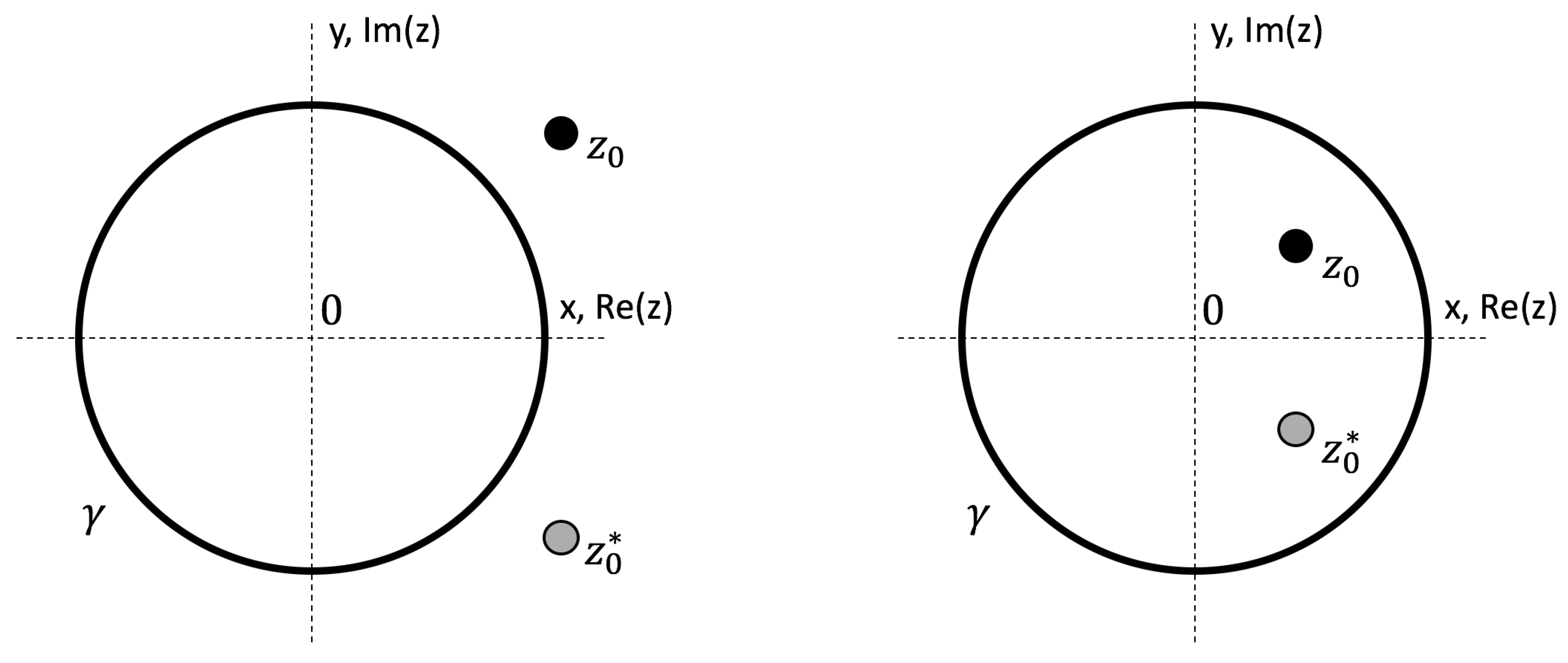
where the latter equality is due to the easily proven general property for circular contour integrals, . The value of (A5) will depend on whether is inside or outside the disk delimited by on the complex plane (see Figure A1). In terms of the original problem, this means that the expressions for inside and outside the solenoid will be different. In the latter case, , meaning that
and
where and . This is the expected result outside the cylinder. On the other hand, inside . Evaluating (A5) in this situation gives
so that
This is the expected result for the transverse component of the vector potential in a finite volume under a constant magnetic field (in this case, a cylinder with ), where .
Figure A1.
Complex plane representation of outside and inside the cylinder.

References
- DeWitt, B. Quantum theory without electromagnetic potentials. Phys. Rev. 1962, 125, 2189. [Google Scholar] [CrossRef]
- Coleman, S. Aspects of Symmetry; Cambridge University Press: Cambridge, UK, 1985. [Google Scholar]
- Faddeev, L.; Jackiw, R. Hamiltonian reduction of unconstrained and constrained systems. Phys. Rev. Lett. 1988, 60, 1692. [Google Scholar] [CrossRef] [PubMed]
- Henneaux, M.; Teitelboim, C. Quantization of Gauge Systems; Princeton University: Princeton, NJ, USA, 1992. [Google Scholar]
- Barbero, G.F.J.; Díaz, B.; Margalef-Bentabol, J.; Villaseñor, E.J.S. Dirac’s algorithm in the presence of boundaries: A practical guide to a geometric approach. arXiv 2019, arXiv:1904.11790. [Google Scholar]
- Jackiw, R. Constrained quantization without tears. In Constraint Theory and Quantization Methods: From Relativistic Particles to Field Theory and General Relativity; Colomo, F., Lusanna, L., Marmo, G., Eds.; World Scientific: River Edge, NJ, USA, 1994; p. 448. [Google Scholar]
- Jackson, J.D. Classical Electrodynamics; Wiley: New York, NY, USA, 1998. [Google Scholar]
- Peskin, M.E.; Schroeder, D.V. An Introduction to Quantum Field Theory; Westview Press: Boulder, CO, USA, 1995. [Google Scholar]
- Feynman, R.P.; Hibbs, A.R. Quantum Mechanics and Path Integrals; McGraw-Hill: New York, NY, USA, 1965. [Google Scholar]
- Aharonov, Y.; Bohm, D. Significance of electromagnetic potentials in the quantum theory. Phys. Rev. 1959, 115, 485. [Google Scholar] [CrossRef]
- Aharonov, Y.; Bohm, D. Further considerations on electromagnetic potentials in the quantum theory. Phys. Rev. 1961, 123, 1511. [Google Scholar] [CrossRef]
- Feynman, R.P.; Leighton, R.B.; Sands, M. The Feynman Lectures on Physics Vol. 2: Mainly Electromagnetism and Matter; Addison-Wesley: Boston, MA, USA, 1979. [Google Scholar]
- Peshkin, M.; Tonomura, A. The Aharonov-Bohm Effect; Springer: Berlin, Germany, 1989. [Google Scholar]
- Sakurai, J.J.; Napolitano, J. Modern Quantum Mechanics; Cambridge University Press: Cambridge, UK, 2017. [Google Scholar]
- Griffiths, D.J. Introduction to Electrodynamics; Prentice Hall: Upper Saddle River, NJ, USA, 1981. [Google Scholar]
- Bjorken, J.D.; Drell, S.D. Relativistic Quantum Fields; McGraw-Hill: New York, NY, USA, 1965. [Google Scholar]
- Vogel, W.; Welsch, D.G. Quantum Optics; John Wiley and Sons: Hoboken, NJ, USA, 2006. [Google Scholar]
- Weinberg, S. Lectures on Quantum Mechanics; Cambridge University Press: Cambridge, UK, 2015. [Google Scholar]
- Calkin, M.G. An invariance property of the free electromagnetic field. Am. J. Phys. 1965, 33, 958–960. [Google Scholar] [CrossRef]
- Deser, S.; Teitelboim, C. Duality transformations of Abelian and non-Abelian gauge fields. Phys. Rev. D 1976, 13, 1592. [Google Scholar] [CrossRef]
- Deser, S. Off-shell electromagnetic duality invariance. J. Phys. A 1982, 15, 1053. [Google Scholar] [CrossRef]
- Agullo, I.; del Rio, A.; Navarro-Salas, J. Electromagnetic duality anomaly in curved spacetimes. Phys. Rev. Lett. 2017, 118, 111301. [Google Scholar] [CrossRef]
- Agullo, I.; del Rio, A.; Navarro-Salas, J. Gravity and handedness of photons. Int. J. Mod. Phys. D 2017, 26, 1742001. [Google Scholar] [CrossRef]
- Agullo, I.; del Rio, A.; Navarro-Salas, J. Classical and quantum aspects of electric-magnetic duality rotations in curved spacetimes. Phys. Rev. D 2018, 98, 125001. [Google Scholar] [CrossRef] [Green Version]
- Agullo, I.; del Rio, A.; Navarro-Salas, J. On the Electric-Magnetic Duality Symmetry: Quantum Anomaly, Optical Helicity, and Particle Creation. Symmetry 2018, 10, 763. [Google Scholar] [CrossRef]
- Stewart, A.M. Role of nonlocality of the vector potential in the Aharonov-Bohm effect. Can. J. Phys. 2013, 91, 373. [Google Scholar] [CrossRef]
- Majumdar, P.; Ray, A. Maxwell Electrodynamics in Terms of Physical Potentials. Symmetry 2019, 11, 915. [Google Scholar] [CrossRef]
Figure 1.
Experimental setup we will consider to analyse the magnetic AB effect. A source of electrons is located at the point , from which one is emitted at a time . Between the source and a screen on the other side of the setup there is a wall, containing two slits A and B, and a long impenetrable cylinder behind it. Inside the cylinder, oriented parallel to the z-axis, there is a magnetic field , while outside . The electrons can trace two types of paths to reach the point on the screen at a time , either above (e.g., ) or below (e.g., ) the cylinder.

© 2019 by the authors. Licensee MDPI, Basel, Switzerland. This article is an open access article distributed under the terms and conditions of the Creative Commons Attribution (CC BY) license (http://creativecommons.org/licenses/by/4.0/).
Share and Cite
MDPI and ACS Style
Bernabeu, J.; Navarro-Salas, J. A Non-Local Action for Electrodynamics: Duality Symmetry and the Aharonov-Bohm Effect, Revisited. Symmetry 2019, 11, 1191. https://doi.org/10.3390/sym11101191
AMA Style
Bernabeu J, Navarro-Salas J. A Non-Local Action for Electrodynamics: Duality Symmetry and the Aharonov-Bohm Effect, Revisited. Symmetry. 2019; 11(10):1191. https://doi.org/10.3390/sym11101191
Chicago/Turabian StyleBernabeu, Joan, and Jose Navarro-Salas. 2019. "A Non-Local Action for Electrodynamics: Duality Symmetry and the Aharonov-Bohm Effect, Revisited" Symmetry 11, no. 10: 1191. https://doi.org/10.3390/sym11101191
Note that from the first issue of 2016, this journal uses article numbers instead of page numbers. See further details here.