Detection of Compound Faults in Ball Bearings Using Multiscale-SinGAN, Heat Transfer Search Optimization, and Extreme Learning Machine

Abstract

Intelligent fault diagnosis gives timely information about the condition of mechanical components. Since rolling element bearings are often used as rotating equipment parts, it is crucial to identify and detect bearing faults. When there are several defects in components or machines, early fault detection becomes necessary to avoid catastrophic failure. This work suggests a novel approach to reliably identifying compound faults in bearings when the availability of experimental data is limited. Vibration signals are recorded from single ball bearings consisting of compound faults, i.e., faults in the inner race, outer race, and rolling elements with a variation in rotational speed. The measured vibration signals are pre-processed using the Hilbert–Huang transform, and, afterward, a Kurtogram is generated. The multiscale-SinGAN model is adapted to generate additional Kurtogram images to effectively train machine-learning models. To identify the relevant features, metaheuristic optimization algorithms such as teaching–learning-based optimization, and Heat Transfer Search are applied to feature vectors. Finally, selected features are fed into three machine-learning models for compound fault identifications. The results demonstrate that extreme learning machines can detect compound faults with 100% Ten-fold cross-validation accuracy. In contrast, the minimum ten-fold cross-validation accuracy of 98.96% is observed with support vector machines.

1. Introduction

Rolling element bearings (REBs) are an essential component in rotating machinery, used frequently in various industrial machinery and equipment. When rotating machinery is operated for a substantial amount of time, wear and tear on the surface of the REBs has been observed. Condition monitoring is beneficial for detecting faults and identifying the state of the structure or components. To detect faults in the bearings, several condition-monitoring techniques, such as acoustic emission, vibration analysis, thermal imaging, etc., have been utilized and reported in the literature [1,2]. Vibration-based condition monitoring effectively detects faults in real-time conditions and detects abrupt changes in machinery conditions [3,4]. When a localized defect arises on the elements of REBs, the faulty rolling surface collides with another surface; therefore, an impulse is generated. Further, due to the varying stiffness observed from operating conditions, vibration signals are non-linear and non-stationary [4,5]. Therefore, choosing an appropriate signal-processing algorithm is a significant challenge. Walsh Hadamard Transform (WHT), Wigner–Ville distribution (WVD), etc, are some signal processing techniques for extracting various statistical features. Zhang et al. [6] applied variational mode decomposition to decompose the vibration signals acquired from various bearing conditions and utilize fractal dimensions to diagnose bearing faults. Gu and Peng [7] proposed a methodology to extract the characteristic information from the bearing fault signals based on ensemble empirical mode decomposition and permutation entropy. In another approach [8], Duan et al. introduced minimum entropy morphological deconvolution to identify the impulses based on the amplitude ratio of the diagonal slice spectrum. The authors compared the simulation and experimental signals and verified the proposed methodology’s effectiveness. However, weak signals and signals acquired from compound faults that are non-stationary are complicated to identify with signal-processing techniques alone.

In the last three decades, machine learning (ML) algorithms are reported as an effective technique for quickly identifying the healthy and abnormal conditions of machinery components [9,10,11]. ML models such as Support Vector Machine (SVM), Artificial Neural Network (ANN), Random Forest, Gradient Boosting, etc. are found to be effective in diagnosing faults in bearings, gears, pumps, etc. Due to the Industrial Internet of Things (IIoT) development and the need to implement Industry 4.0, an enormous amount of data is required. It is observed that during operation, the vast majority of monitoring data are healthy, and significantly few faulty data are available to train ML models [12]. As a result, fault identification and diagnosis with the availability of limited fault sample signals are critical [13,14]. Generative adversarial network (GAN) emerges as a superior technique to efficiently deal with the imbalanced data, due to the machinery’s operating condition restrictions. GAN was proposed by Goodfellow in 2014 [15] and is considered as an unsupervised generative neural network. GAN comprises a generator (G) and discriminator (D) network that may construct additional samples from various fault conditions. Recently, various authors have explored the GAN-based fault diagnosis methodology. Gao et al. [16] developed a methodology combining GAN with a convolution neural network to diagnose faults in rolling element bearings. Lee et al. [17] successfully applied GAN in an induction motor to generate fault data to overcome the issue of data imbalance. It is reported that the GAN-based fault diagnosis methodology is applied to the 2D representation of signals, i.e., either spectrogram or scalogram, which reveals the tool-wear conditions [18]. To accurately determine the status of components, various image quality parameters need to be extracted from either the spectrogram or scalogram and later used for constructing feature vectors. Recent literature suggests that feature selection techniques can influence fault detection accuracy [19,20]. Li et al. [21] explore maximum relevance and minimum redundancy (mRMR) criteria to identify the optimal feature subset, which improves the accuracy of identifying various gear faults. In another study, a feature selection criterion based on optimized Weighted Kernel Principal Component Analysis was proposed by Shen and Xu [22] to diagnose bearing failures.

Although considerable studies have been reported in fault diagnosis using GANs or conventional feature selection criteria, the issue of effectively predicting compound defects with limited experimental data still needs to be addressed. Therefore, the primary goal of our proposed study is to provide an appropriate methodology for reliably detecting compound faults in bearings. In addition, the authors have explored teaching–learning-based optimization (TLBO) and Heat Transfer Search (HTS) metaheuristic techniques to identify the best feature subset which identify compound faults effectively. As per the study conducted by the authors, TLBO and HTS feature-selection strategies are not being effectively explored for fault diagnosis. Motivated by the facts mentioned above, the significant contributions of the proposed methodology are as follows:

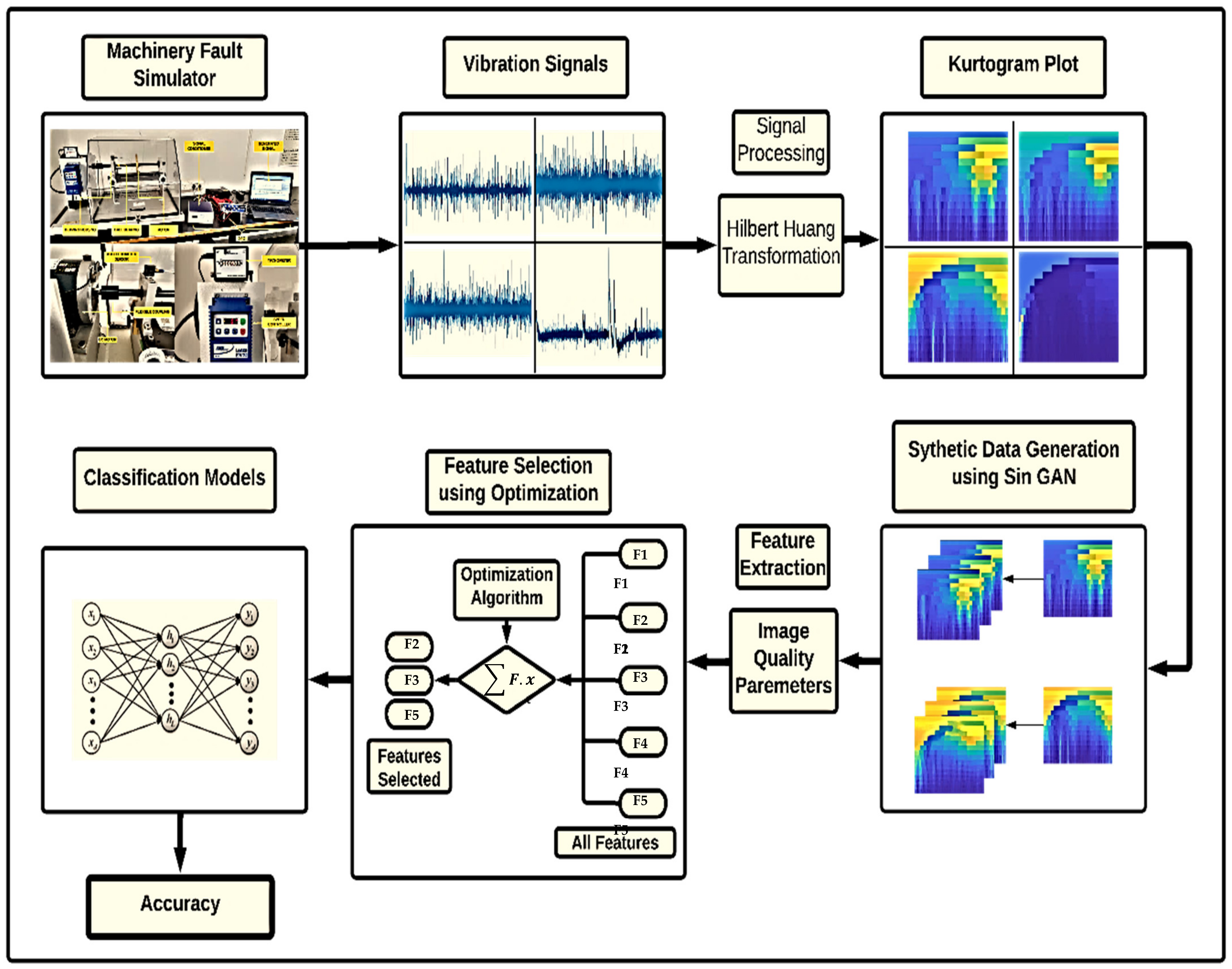
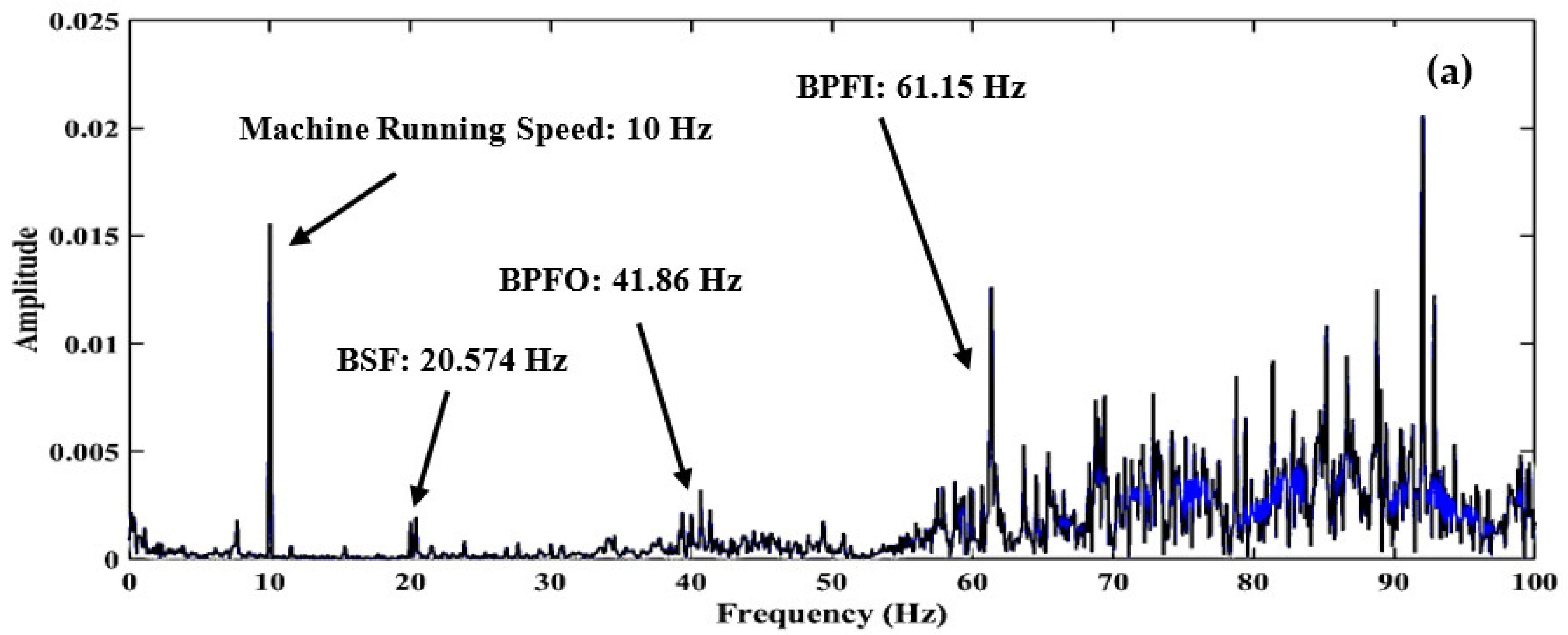
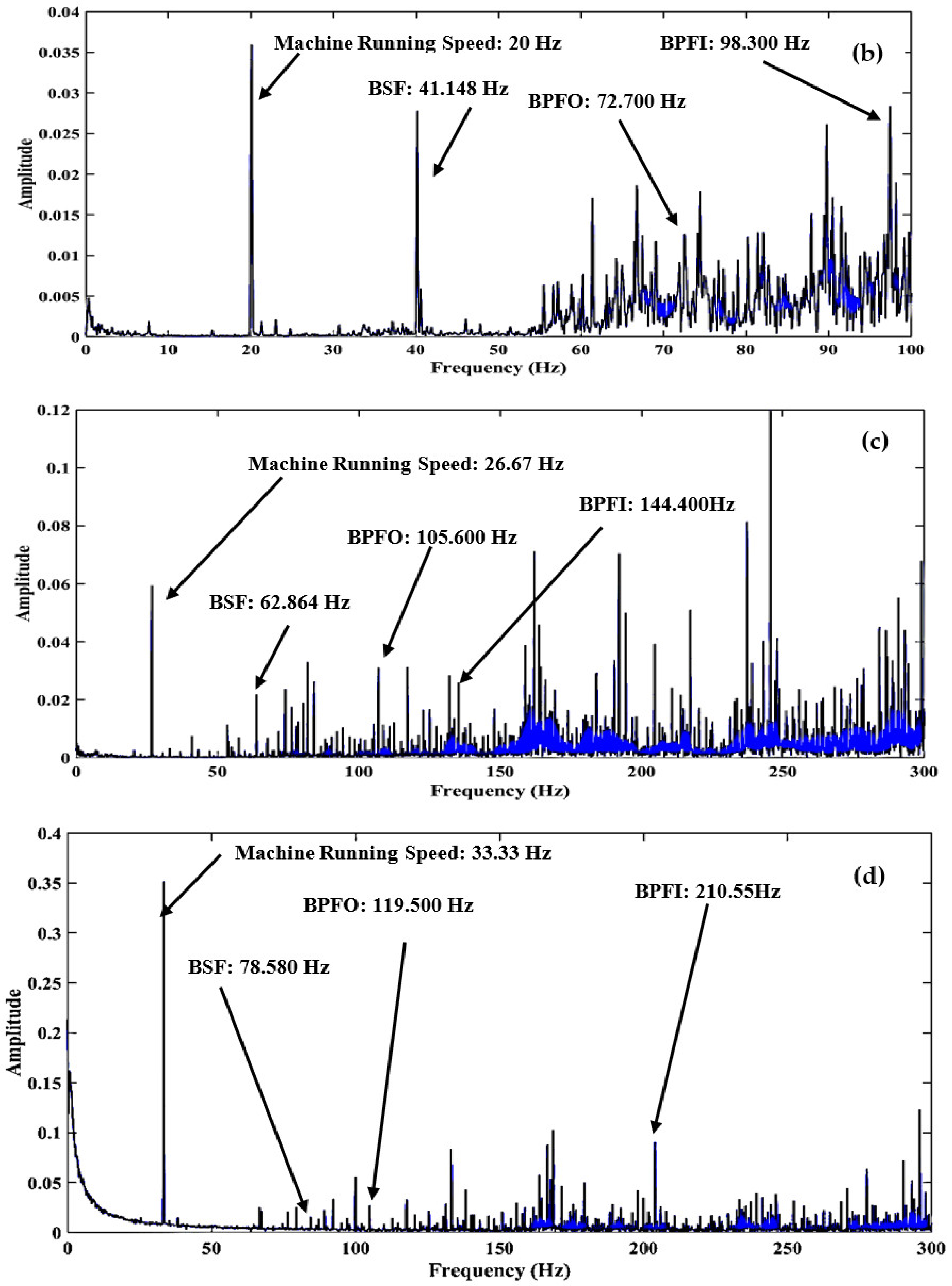
• Experiments were conducted to capture signals from compound faults, i.e., Inner Race Defect (IRD), Ball Defect (BD), and Outer Race Defect (ORD) in a single rolling element bearing with a variation in the rotational speed of the shaft.
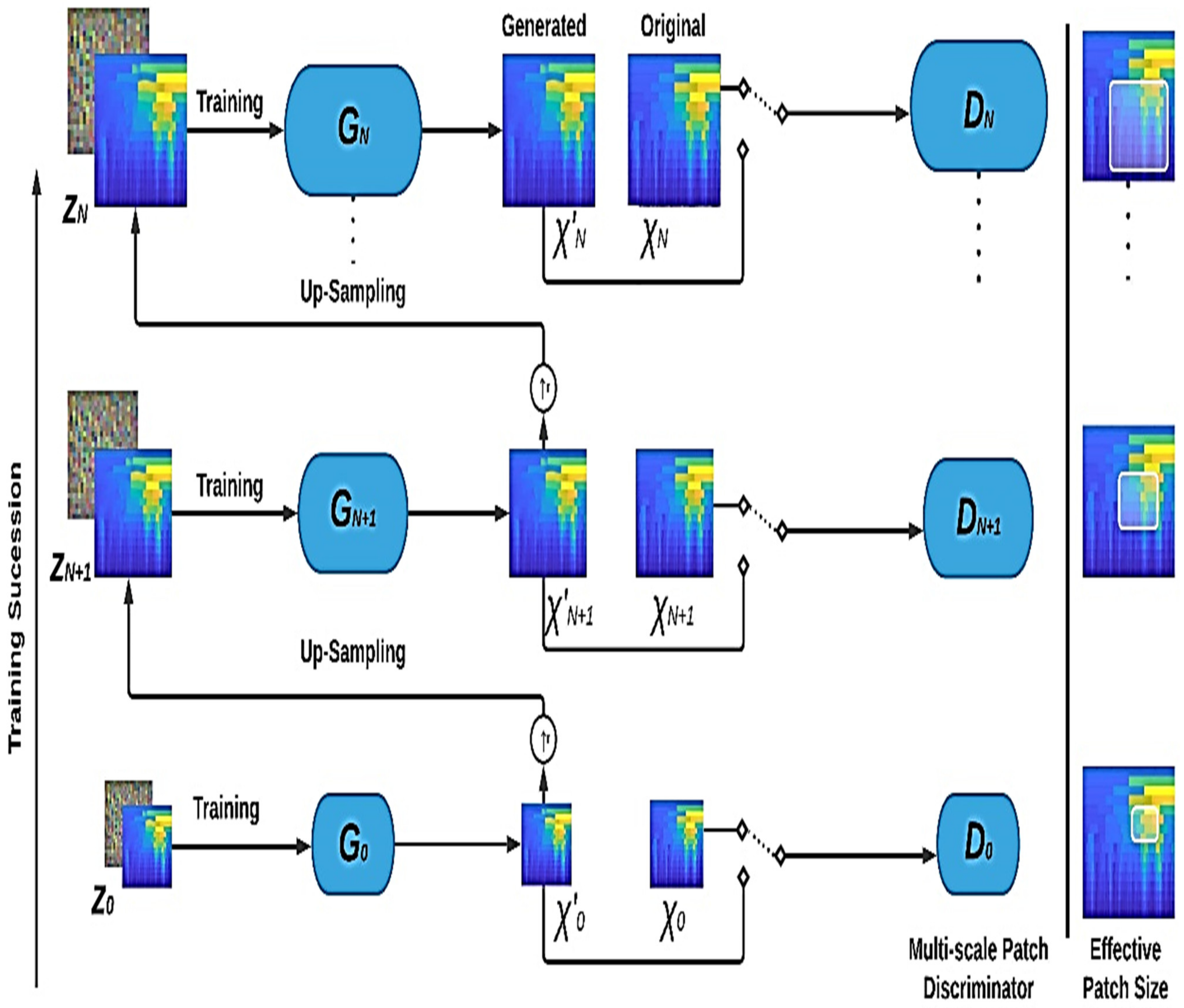
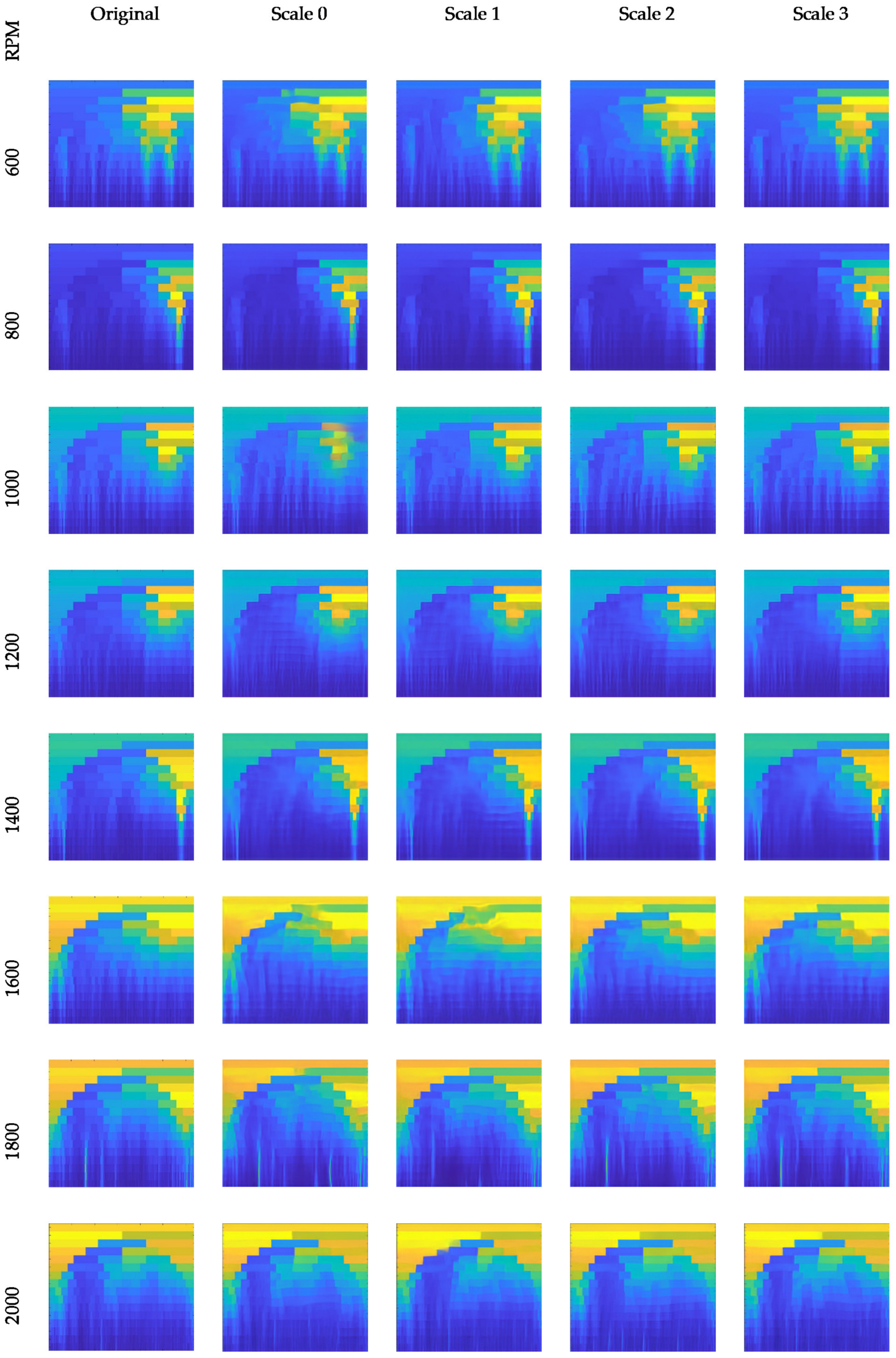
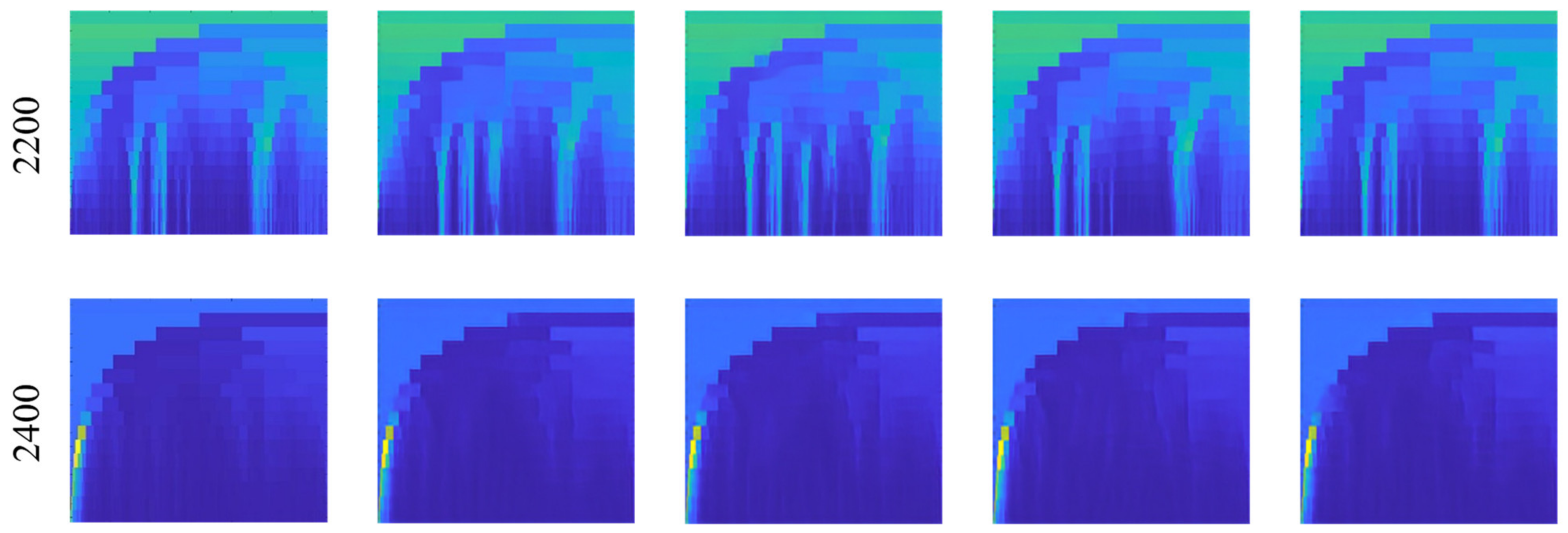
• To effectively develop machine-learning models, many images are required. Therefore, recently developed Multi-Scale Single Image Generative Adversarial Network (Multiscale-SinGAN) is utilized.
• TLBO and HTS metaheuristic algorithms were adapted and applied to select the optimal feature subset.
• The optimized features subset is evaluated with three classifiers, i.e., Support Vector Machine (SVM), Standardized Variable Distance (SVD), and Extreme Learning Machine (ELM), with 30% hold-out and ten-fold cross-validation accuracy to detect compound faults.

The remaining work is organized as follows: Section 2 briefly discusses the Hilbert–Huang transform, the Multiscale-SinGAN architecture model, the TLBO and HTS metaheuristic optimization algorithms, ML algorithms, and experimentation and feature extraction. In Section 3, the results are discussed in a comprehensively manner. Finally, the outcomes are summarized in Section 4. Figure 1 shows the methodology of compound fault detection in bearings using Multiscale-SinGAN and metaheuristic feature selection.

2. Materials and Methods

2.1. Hilbert–Huang Transform

The Hilbert–Huang transform (HHT) is a non-linear signal processing technique that involves two steps. In the first stage, signals are broken down into various intrinsic mode functions (IMFs) and, in second stage, the extracted IMFs are subjected to the Hilbert Transform, which generates an orthogonal pair. The instantaneous fluctuations in amplitudes and frequencies can be determined from the corresponding IMF and its orthogonal pair. As a result, HHT is highly beneficial for extracting useful information from non-linear time series data, such as bearing and gear faults [23]. The steps required to implement HHT are as follows:

For any signal, $a\left(\gamma \right)$ of Lp class, its Hilbert transform b(t) is given by

$$b\left(t\right)=\frac{C}{\pi }{{\displaystyle \int }}_{-\infty }^{+\infty }\frac{a\left(\gamma \right)}{t-\gamma }d\gamma$$

(1)

where C represents Cauchy singular integral value.

The analytic function when Hilbert transform b(t) is applied to function a(t) is represented as

$$d\left(t\right)=a\left(t\right)+ib\left(t\right)=x\left(t\right)e^{i\theta \left(t\right)}$$

(2)

$$x\left(t\right)={(a^2+b^2)}^{\raisebox{1ex}{$1$}\!\left/ \!\raisebox{-1ex}{$2$}\right.} , \theta \left(t\right)={\tan }^{-1}\frac{b}{a}$$

(3)

Here, a represents instantaneous amplitude, and θ represents instantaneous phase function. The instantaneous frequency is calculated as

$$\omega \left(t\right)=\frac{d\theta \left(t\right)}{dt}$$

(4)

The amplitude can be expressed as a function of frequency and time, h (ω, t), which can be formulated as:

$$s\left(\omega \right)={{\displaystyle \int }}_0^{T}h\left(\omega ,t\right)dt$$

(5)

2.2. Multiscale-SinGAN

GAN is considered as unsupervised algorithm which Goodfellow proposed in 2014. Generative adversarial networks (GANs) are beneficial for industrial applications where there is a lack of annotated data that can be used to train machine-learning algorithms on both healthy and faulty data. GANs consist of two models, a generator ‘G’ and discriminator ‘D’, which are trained simultaneously. A well-trained GAN model can generate additional images after applying a minimax formulation between two subnetworks—the discriminator ‘D’ and the generator ‘G’. Mathematically, the equation is represented as follows [24]:

$$mi{n}_{G}ma{x}_D\left(D,G\right)=E_{x~Pdata}\left[Log D \left(x\right)\right]+E_{x~Pz}[Log\left(1-D\left(G\left(z\right)\right)\right]$$

(6)

where D(x) represents the likelihood that the input image x is generated by augmented data rather than real data, while G(z) represents generated data. P_z is a noise distribution, and E is the expectation of a variable in Equation (6).

The SinGAN, which only needs one image to train, was first introduced by Shaham et al. [24]. SinGAN captures and analyses the intrinsic association between training images and can also capture color and texture information. It has a pyramidal structure of similar ‘N’ GAN networks. Initially, at the coarse scale ‘0’, SinGAN focuses on global features like shape and image alignment. As the training continues, it compensates for local features such as texture, edge information, etc., at a finer scale ‘n’. Initially, images are generated by upsampling from previous scales χ’N+1 and putting them into a new map Z_N. Afterward, a residual image is returned to (χ’N+1) ↑r after being passed through convolution layers. Figure 2 shows the SinGAN architecture.

2.3. Metaheuristic Optimization Algorithms

Metaheuristic algorithms are a promising technique and are successfully utilized in different domains. For instance, most engineering optimization issues need solutions to multi-objective issues since they are substantially non-linear. On the other hand, it is challenging to design the optimization issue to solve for optimality when dealing with artificial-intelligence and machine-learning challenges, which largely depend on enormous datasets. As a result, metaheuristics are crucial in helping to resolve practical issues that are difficult to resolve using traditional optimization techniques. A metaheuristic algorithm searches for a satisfactory solution to a complicated, hard-to-solve optimization issue. In the methodology proposed, the authors explored the utility of teaching–learning-based optimization (TLBO) and Heat Transfer Search (HTS) optimization techniques to identify the optimal feature subset. Details of both algorithms are discussed in the next subsection.

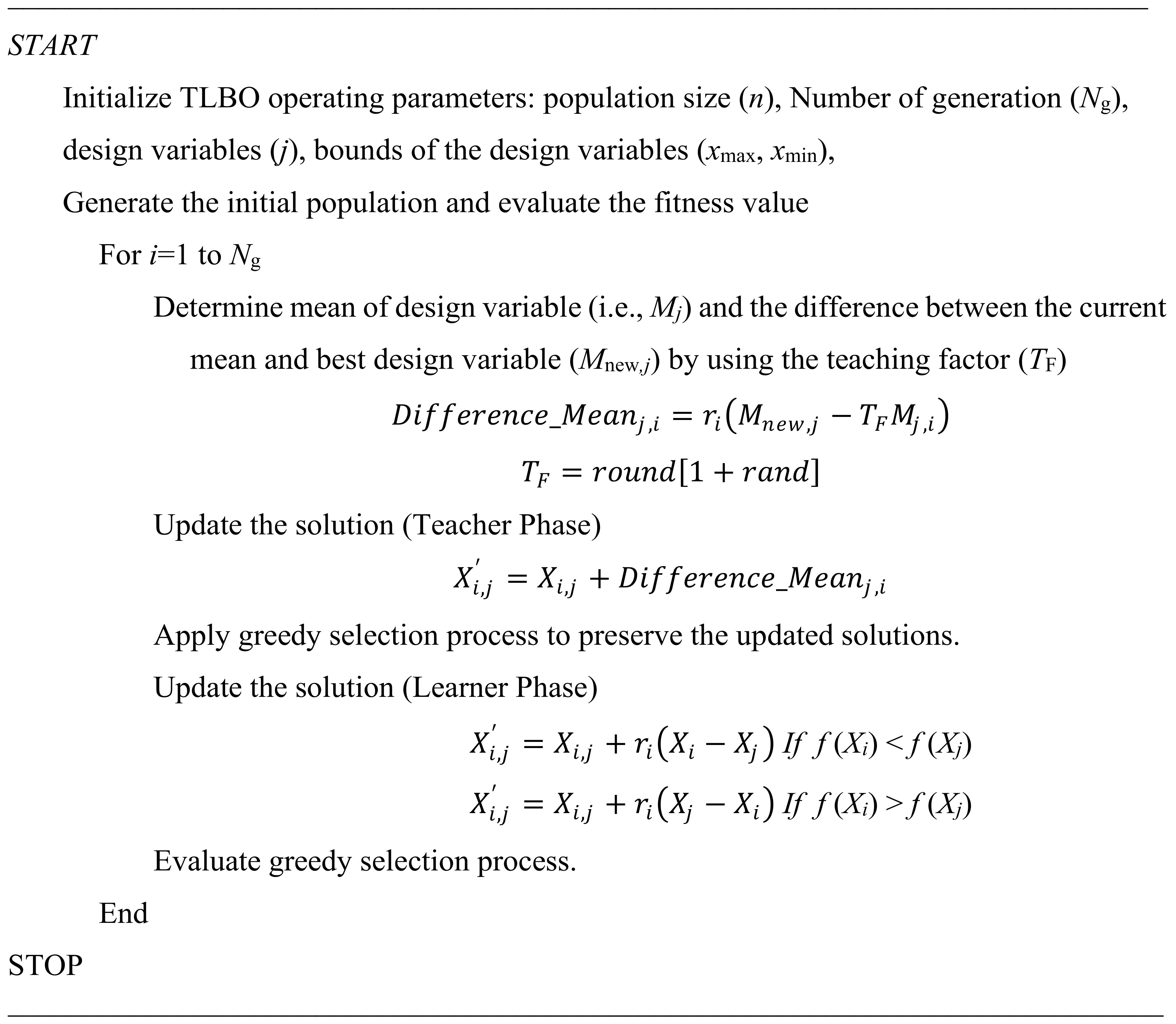
2.3.1. Teaching–Learning-Based Optimization (TLBO) Algorithm

The TLBO algorithm designed by Rao et al. [25,26] examines the impact of a teacher’s influence on the upshot of the student’s performance in a classroom. The teaching–learning approach is designed to improve the student’s performance by learning from teachers and other students (result). The TLBO algorithm is executed in two phases to improvise/update the solution. The algorithm initiates with a random generation of ‘n’ solution. The solution is then obtained in successive stages through the generation of different phases of teaching and learning. In the teacher phase, the solution is updated with the help of the best solution and mean solution of population. The teacher phase tries to improve the mean solution for the entire population. In the learner phase, the solution is updated from randomly selected solutions through the population. The pseudocode of the TLBO algorithm is presented in Figure 3.

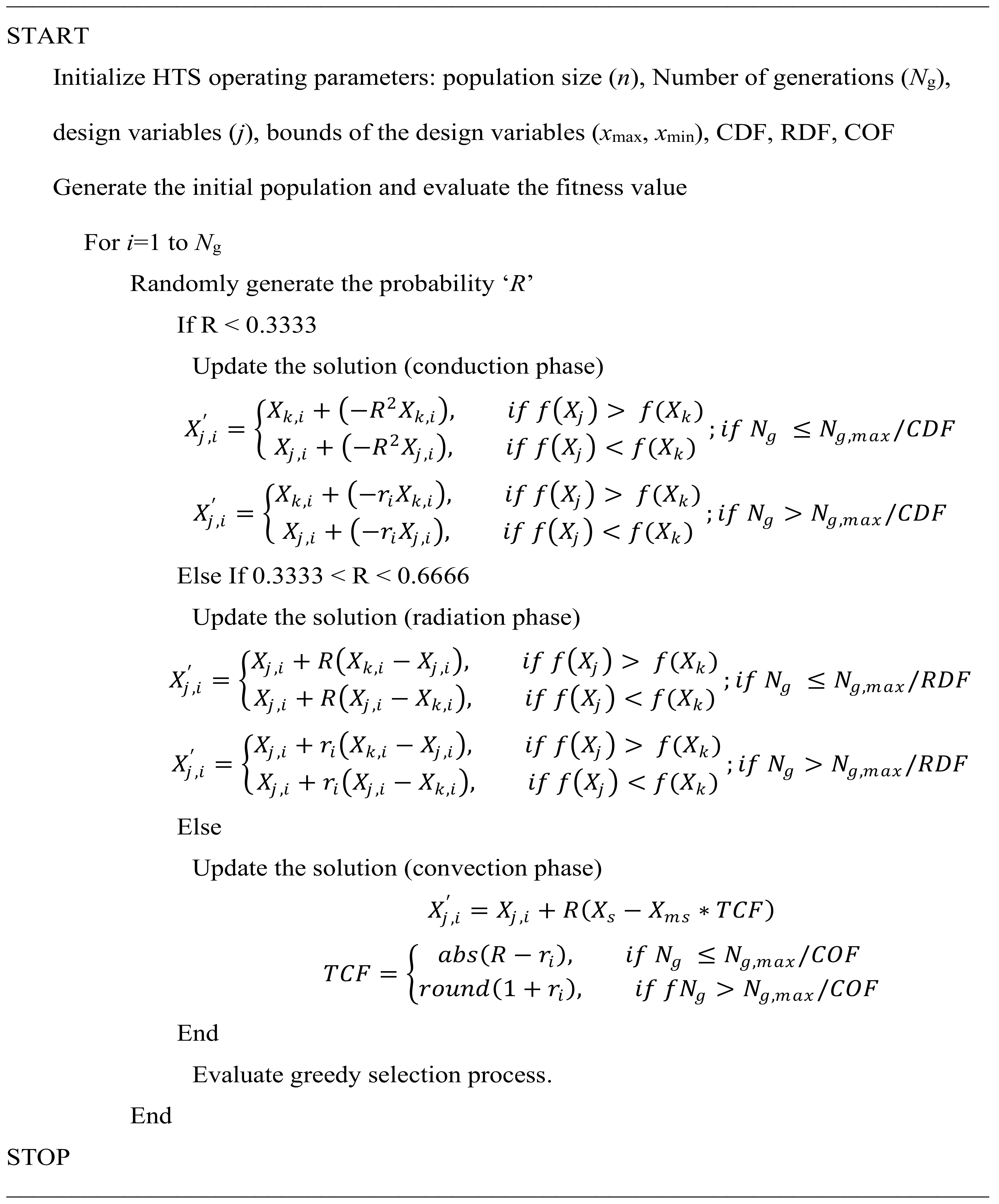
2.3.2. Heat Transfer Search (HTS) Algorithm

The HTS algorithm, presented by Patel and Savsani [27], resembles the heat transfer behavior between the system and its surrounding. The HTS algorithm is executed in three stages (conduction, convection, and radiation phase) to improvise/update the solution. The algorithm initiates with a random generation of ‘n’ solution. In the subsequent stage, the solution is updated through a randomly selected heat transfer phase in each generation. The solution is updated in the conduction and radiation phase with a randomly selected solution from the population. However, the mechanism to update the solution differs in both phases. In the convection phase, the solution is updated based on the best population solution. Further, all three phases have two different search mechanism, which is governed by control parameters called conduction factor (CDF), convection factor (COF), and radiation factor (RDF). Two different search mechanisms of each phase balance the exploration and exploitation throughout the optimization procedure. The pseudocode of the HTS algorithm is presented in Figure 4.

2.4. Machine-Learning Algorithms

Classification and regression are two preliminary tasks of machine-learning algorithms. Labels are predicted in classification, whereas numerical values are predicted in regression. Bearing fault detection requires labels to predict various fault conditions, whereas regression analysis is required to detect fault severity. In this study, the authors investigated the prediction capability of the SVM, ELM, and SVD ML models to effectively detect the compound fault in bearings at various rpm.

2.4.1. Support Vector Machine

SVM is a form of the supervised algorithm based on its better generalization capability and versatility in handling a variety of applications. Cortes and Vapnik developed a basic model of SVM in 1994, which is capable of handling both classification and regression problems with multiple continuous and categorical variables [28]. A Support Vector Machine classifies data by locating the hyperplane with the most significant margin between two classes. The support vectors are the vectors (cases) that define the hyperplane. An ideal SVM analysis should produce a hyperplane that completely separates the vectors into two non-overlapping classes. However, perfect separation may not be possible, or it may result in a model with many cases that it needs to classify correctly. In this situation, SVM finds the hyperplane that maximizes the margin and minimizes the misclassifications. Kernel-based SVM has received much attention due to its capability to handle nonlinear data efficiently and make data more separable. Mathematically, the formation of a hyperplane as an optimization function can be represented as [29]:

$$\mathrm{Min}\frac{1}{ 2}{w}^2+C{\sum }_{i=1}^K{\xi }_i$$

(7)

$$\mathrm{Subjected} \mathrm{to}\{ y_i\left(w^T{x}_i+b\right)\ge 1-{\xi }_i$$

(8)

$${\xi }_i\ge 0, i=1,2,\dots K$$

where C is known as the error penalty and ${\xi }_i$ represents the slack variable.

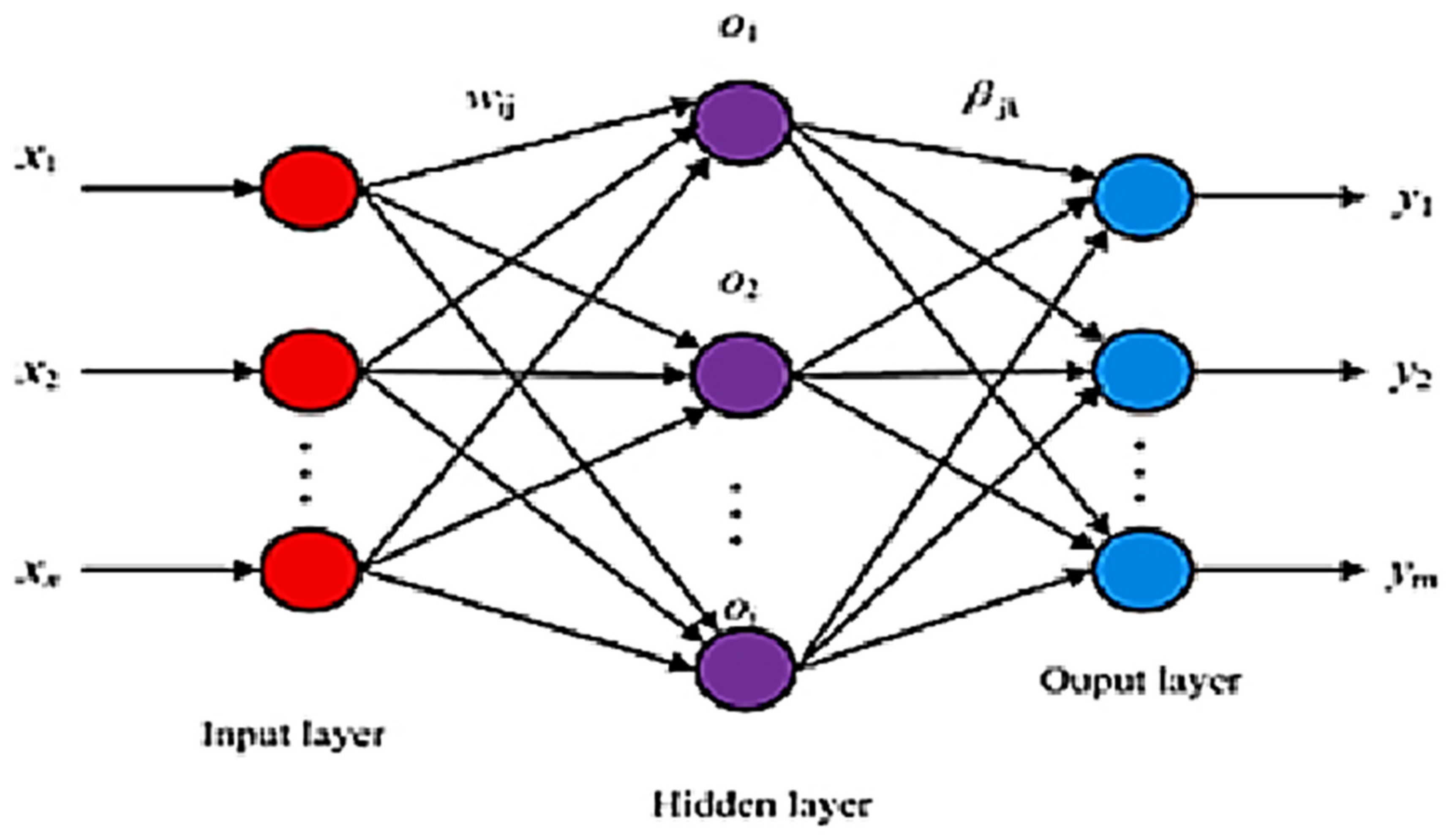
2.4.2. Extreme Learning Machine

Extreme Learning Machine (ELM) was introduced by Huang et al. [30]. The learning rate of feed-forward neural networks is likely to be slower than necessary. For decades, this constraint has been a significant hurdle in many applications. Unlike traditional learning procedures, a learning strategy is proposed based on Single-Hidden-Layer Feed-Forward Neural Networks, known as Extreme Learning Machine (ELM). In most cases, the weights of hidden nodes are usually learned in a single step which results in a fast-learning scheme as shown in Figure 5. ELM allocates hidden nodes randomly and uses least-squares techniques to estimate the output weights [31]. In ELM, the objective function with Q hidden node for a single hidden layer is represented as [32]:

$$f_Q={{\displaystyle \sum }}_{i=1}^Q{\beta }_i{h}_i{\beta }_{i}y$$

(9)

where β_i = output weight, i = number of hidden nodes, and h_i = output value of hidden node.

$$h_{i}y=D{a}_i,b_i,y$$

(10)

where $a_i$ and $b_i$ = parameters of hidden node.

For N number of samples, the output value of the hidden layer is:

$$H=\begin{array}{c}h{y}_1\\ ⋮\\ h{y}_n\end{array}=\begin{array}{ccc}D{a}_1,b_1,y_1& \dots & D{a}_1,b_1,y_1\\ ⋮& ⋮& ⋮\\ D{a}_1,b_1,y_N& \dots & D{a}_1,b_1,y_N\end{array}$$

(11)

The objective matrix used in ELM is represented by T, which incorporates various fault conditions represented by O, and is written as:

T = O₁, O₂ ……… O_N

(12)

The output weight is computed by

$${\beta }_i: {\beta }_i=H^{\phi }T$$

(13)

Finally, the classification can be computed as:

$$Label y_{proc}=argmax f_Q y_{proc}$$

(14)

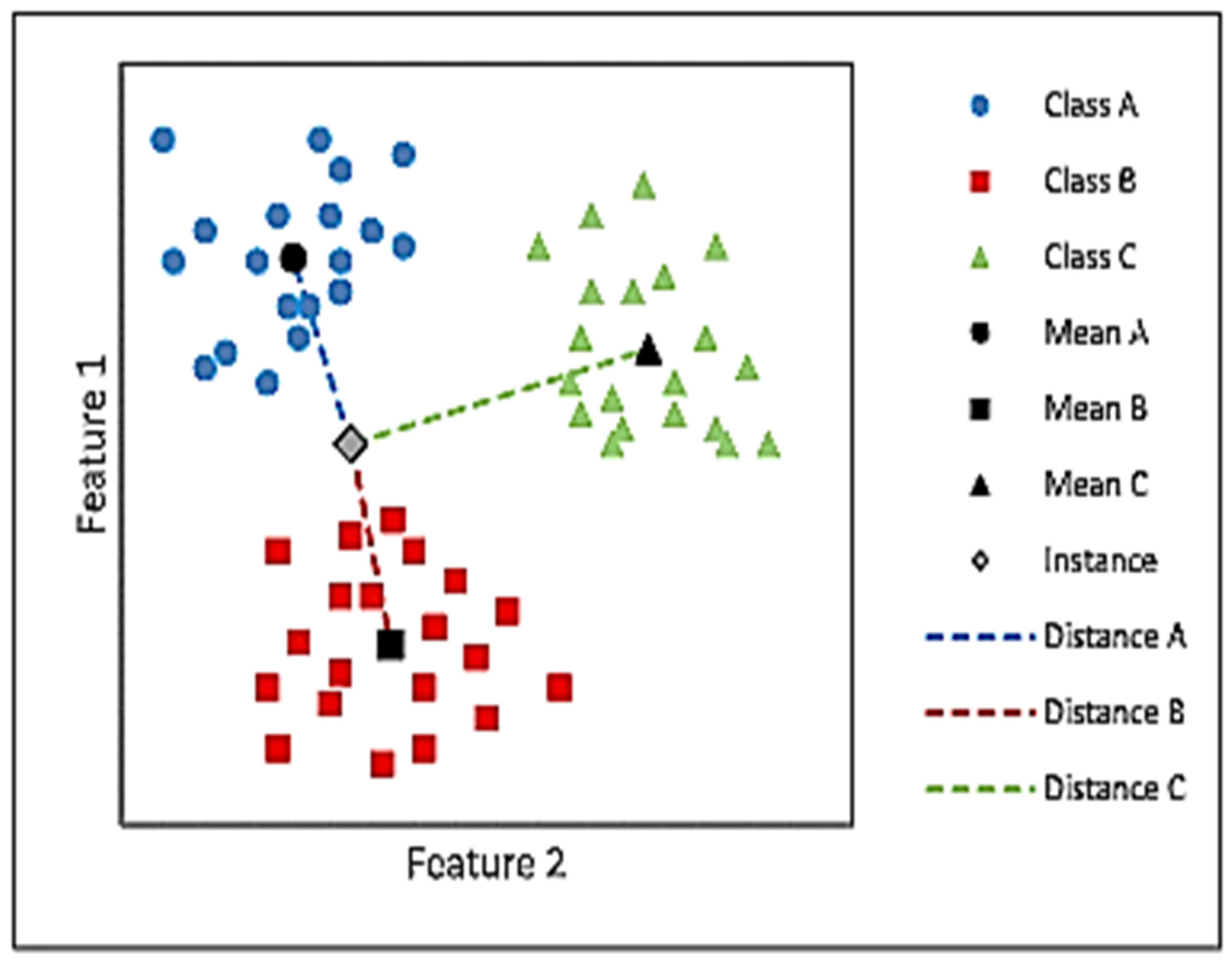
2.4.3. Standardized Variable Distance

The Standardized Variable Distance (SVD) classifier is formulated based on the Minimum Distance Classifier (MDC) algorithm principle. Since MDC does not consider the effect of noise while computing the distances of input vectors to the class centroid, it is therefore considered an insensitive variance method. To alleviate this issue, a variance-sensitive model is developed by Aelen and Avuclu [33], known as SVD, which calculates the z-score of an input feature vector. The absolute value of the z-score indicates how many standard deviations are away from the mean. In multiclass classifiers, each input vector belongs to an individual class and is fed to the ML model for training. Based on training from input data, a model is formulated which can be helpful for classification or regression analysis. Equation (15) shows the input matrix (V_x ∈ R^m×n) and the output matrix (V_y ∈ R^m) corresponding to each input vector.

$${\vartheta }_x=\left[\begin{array}{ccc}{X}_{0,0}& \cdots & X_{0,n}\\ ⋮& \ddots & ⋮\\ X_{m,0}& \cdots & X_{m,n}\end{array}\right] , {\vartheta }_{\gamma }=\left[\begin{array}{c}{y}_0\\ ⋮\\ y_m\end{array}\right]$$

(15)

where m represents the number of samples in the data set, and n represents the number of attributes in a dataset. The output vector, which consists of the dataset needed to be trained, is utilized to determine the class labels for the classes, as indicated in Equation (16).

$$\begin{array}{c}{\vartheta }_{\gamma }=\left[y_0,y_1,\dots ,y_m\right]\\ c=\left\{{\exists }_a\in {\vartheta }_{\gamma }:\left(P\left(a\right) ᴧ {\forall }_b\in {\vartheta }_{\gamma }:P\left(b\right)\to a=b\right)\right\}\end{array}$$

(16)

where c represents the number of classes present in dataset. With the help of the z-score, the similarity scores of each input vector are found. If a z-score equals zero, the centroid-class vector has the same value as the sample presented [33]. Figure 6. shows the classification architecture with SVD.

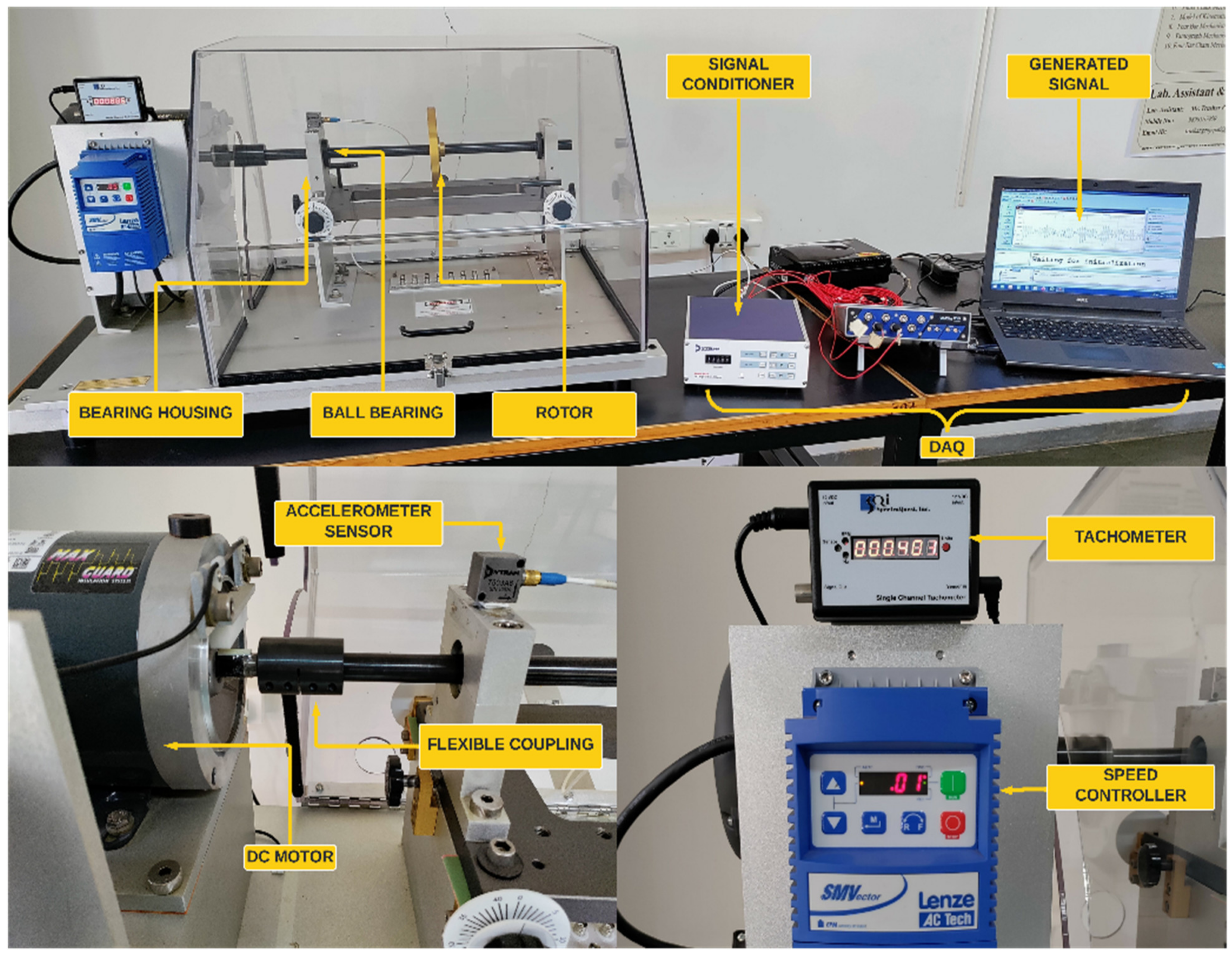
2.5. Experimentation and Kurtogram Extraction

The experimentation is conducted on Machinery Fault Simulator (MFS) to acquire the vibration-based compound fault signals of REBs from the accelerometer. The MFS simulator, as shown in Figure 7, is capable of conducting experiments and acquiring vibration signals at different shaft RPMs and with machinery components, such as a defect in ball bearing, shaft defects, rotor defects, etc. The setup consists of a 1HP AC motor with a multi-featured front panel programmable controller, a piezoelectric accelerometer to capture signals, flexible or rigid coupling, and a data acquisition system with supporting hardware and software. An SKF 6004 Open Deep Groove Ball Bearing with compound faults and a bore diameter of 20 mm, an outer diameter of 42 mm, and a width of 12 mm is mounted on MFS to conduct experiments.

The faults introduced in a single bearing are inner race defect (IRD), an outer race defect (ORD), and a ball defect (BD); therefore, it is referred to as a compound fault. Compound fault bearing used in our study is shown in Figure 8. Seeded point faults of 0.5 mm width and 0.2 mm depth have been introduced in the ball bearing dataset. A radial load of 11 lb (5 kg) is applied on Machinery Fault Simulator with grease lubrication. As a first step, the machine was run with a healthy bearing to establish the baseline data. Signals were captured with variations in shaft speeds of 600–2400 RPM with an interval of 200 RPM. The sampling frequency is set to 12.4 kHz. Since the bearing consists of compound faults, it is challenging to differentiate them solely from vibration signals. Therefore, FFT plots are shown in Figure 9a–d as graphical illustrations, which identify the peaks corresponding to a fault in the inner race, outer race, and ball. In Figure 9, BPFO, BPFI, and BSF represent the ball pass frequency at the outer race, ball pass frequency at the inner race, and ball spin frequency. Detection of faults when fault size is small and when multiple faults are present is tedious and complex. There are several methods to filter the raw vibration signals but HHT is preferable to the wavelet approach because it can remove spurious harmonics that have no underlying physical mean. In addition, HHT is better than the wavelet method because it is faster and is able to detect weak signals with good accuracy. The authors applied HHT on raw vibration signals, and with filter signals, the Kurtogram is generated. Since only 10 Kurtogram are generated, the training and development of the ML model are tedious; therefore, SinGAN is applied to generate additional Kurtogram images. In our study, the authors have generated 2000 Kurtogram images from original images, when the scale in SinGAN is varied from ‘0’ to ‘3’. Original and synthetic images are shown in Figure 10 at various RPM.

3. Results and Discussion

The Python 3, TensorFlow 1.9.1 programming framework is utilized for developing the SinGAN model. The images are processed through the Google COLAB Pro+ online server which gives access to a 52 GB RAM processor with which to process images. As mentioned earlier, from a single Kurtogram image at each scale, 50 images are generated. Since the scale is varied from ‘0’ to ‘3’, corresponding to each original image, 200 augmented images are generated. Finally, a data set of 200 × 10 = 2000 Kurtogram images are constructed. It is generally challenging to classify augmented/generated images from machine-learning models; therefore, standard image quality parameters (IQP) are extracted to construct a feature vector, listed in

Table 1. IQP features extracted from Kurtogram.

Image Quality Parameters	Formula
Mean-Square Error (MSE)	$MSE=\frac{{\sum }_{i=1}^x{\sum }_{j=1}^y({\left[J_1\left(x,y\right)-J_2\left(x,y\right)\right]}^2}{xy}$
Peak Signal-to-Noise Ratio (PSNR)	$PSNR=10{\log }_{10}\left(\frac{V^2}{MSE}\right)$
Signal-to-Noise Ratio (SNR)	$SNR=20{\log }_{10}\frac{S}{N}$
Structural Similarity Index for Measuring Image Quality (SSIM)	$SSI{M}_y=\frac{\left(2{\mu }_X{\mu }_Y+A_1\right)\left(2{\sigma }_{XY}+A_2\right)}{\left({\mu }_A^2+{\mu }_B^2+A_1\right)\left({\sigma }_A^2+{\sigma }_B^2+A_2\right)}$
Multi-Scale Structural Similarity Index for Measuring Image Quality (MSSIM)	$MSSIM \left(J_1,J_2\right)=\frac{{\sum }_{j=1}^{X}SSIM\left(J_{1j},J_{2j}\right)}{J_1}$
2-D Correlation Coefficient	$R=\frac{{\sum }_x{\sum }_y\left(M_{xy}-\overline{M}\right)\left(N_{xy}-\overline{N}\right)}{\sqrt{\left({\sum }_x{\sum }_y{\left(M_{xy}-\overline{M}\right)}^2\right)\left({\sum }_x{\sum }_y{\left(N_{xy}-\overline{N}\right)}^2\right)}}$
2-D Standard Deviation	${\sigma }_y=\sqrt[2]{\frac{{\sum }_{j=1}^x{\left(y_i-\overline{y}\right)}^2}{x-1}}$
Entropy	$E\left(x\right)=-{\displaystyle \sum _{i=1}^N}{x}_i lo{g}_2 x_i$
Blind/Referenceless Image Spatial Quality Evaluator (BRISQUE)	BRISQUE is a model that does not require transformations and instead calculates its characteristics from the image pixels. It is used to assess the quality of a picture by comparing it to a model with the same sort of distortion. With a lower BRISQUE score, higher perceptual quality can be achieved.
Natural Image Quality Evaluator (NIQE)	To determine the no-reference image quality score, NIQE can estimate image quality with arbitrary distortion, despite being trained on immaculate photos. The perceived quality improves when NIQE decreases.
Perception-Based Image Quality Evaluator (PIQE)	PIQE computes the quality score by evaluating block distortion and calculating the local variance of perceptibly distorted blocks.

. The authors computed 11 IQP features from each Kurtogram image, and sample feature vectors are shown in

Table 2. Sample IQP feature vector.

S.No	MSE	PSNR	SNR	SSIM	MSSIM	BRISQUE	NIQE	PIQE	2-D Corr.	2-D Std Dev.	Entropy	Class
1	63.58	−18.03	23.50	0.37	0.65	36.12	7.06	64.31	0.98	36.27	7.37	0
2	80.40	−19.05	22.48	0.35	0.66	33.12	7.96	65.57	0.97	35.25	7.25	0
3	42.16	−16.25	25.28	0.38	0.69	40.13	6.15	65.52	0.98	35.79	7.31	0
4	45.06	−16.54	24.99	0.39	0.69	43.00	6.93	64.01	0.98	35.08	7.33	0
5	49.04	−16.91	24.62	0.39	0.70	37.48	8.07	65.53	0.98	36.15	7.34	0
6	68.41	−18.35	23.18	0.35	0.64	31.37	6.63	65.30	0.97	35.26	7.25	1
7	12.32	−10.90	28.74	0.42	0.75	40.76	6.48	61.96	0.99	29.33	7.08	1
8	19.23	−12.84	26.80	0.37	0.69	41.52	6.65	66.11	0.99	29.03	7.08	1
9	17.52	−12.44	27.20	0.37	0.67	38.66	6.95	64.58	0.99	28.57	7.07	1
10	20.05	−13.02	26.62	0.37	0.69	42.00	6.56	62.55	0.99	29.14	7.05	1
11	9.84	−9.93	28.11	0.28	0.69	30.56	7.24	63.83	0.99	20.43	6.39	9
12	9.85	−9.94	28.11	0.28	0.69	31.55	7.08	63.46	0.99	20.42	6.38	9
13	9.89	−9.95	28.09	0.28	0.69	28.32	7.31	61.63	0.99	20.42	6.39	9
14	9.89	−9.95	28.09	0.28	0.70	30.21	6.37	63.16	0.99	20.42	6.39	9
15	9.93	−9.97	28.07	0.28	0.70	29.52	5.76	62.87	0.99	20.43	6.39	9

. It is observed that the computation cost and biasedness in classification are increased by the presence of redundant and irrelevant features, which significantly affects the classification accuracy. Therefore, feature-selection techniques such as feature ranking and metaheuristic optimization algorithms are needed to enhance classification accuracy. To select the relevant features, TLBO and HTS metaheuristic optimization algorithms are applied on the extracted IQP features, and the optimized features are mentioned in

Table 3. Sample features selected using TLBO optimization.

S. No	SNR	2-D Corr.	2-D Std Dev.	Entropy	Class
1	36.12	7.06	0.98	36.27	0
2	33.12	7.96	0.97	35.25	0
3	40.13	6.15	0.98	35.79	0
4	43.00	6.93	0.98	35.08	0
5	37.48	8.07	0.98	36.15	0
6	31.37	6.63	0.97	35.26	1
7	40.76	6.48	0.99	29.33	1
8	41.52	6.65	0.99	29.03	1
9	38.66	6.95	0.99	28.57	1
10	42.00	6.56	0.99	29.14	1
11	30.56	7.24	0.99	20.43	9
12	31.55	7.08	0.99	20.42	9
13	28.32	7.31	0.99	20.42	9
14	30.21	6.37	0.99	20.42	9
15	29.52	5.76	0.99	20.43	9

and

Table 4. Sample features selected using HTS optimization.

S.No	BRISQUE	NIQE	2-D Corr.	2-D Std Dev.	Class
1	23.50	0.98	36.27	7.37	0
2	22.48	0.97	35.25	7.25	0
3	25.28	0.98	35.79	7.31	0
4	24.99	0.98	35.08	7.33	0
5	24.62	0.98	36.15	7.34	0
6	23.18	0.97	35.26	7.25	1
7	28.74	0.99	29.33	7.08	1
8	26.80	0.99	29.03	7.08	1
9	27.20	0.99	28.57	7.07	1
10	26.62	0.99	29.14	7.05	1
11	28.11	0.99	20.43	6.39	9
12	28.11	0.99	20.42	6.38	9
13	28.09	0.99	20.42	6.39	9
14	28.09	0.99	20.42	6.39	9
15	28.07	0.99	20.43	6.39	9

. However, it is impossible to distinguish healthy and faulty conditions only by simply looking at the feature vector; hence, machine learning models are needed to differentiate the bearing condition.

Three ML models (SVM, ELM, and SVD) are considered to demonstrate the utility of the proposed framework of compound fault prediction. To evaluate the individual capabilities of a prediction model, standard performance metrics (accuracy, precision, recall, and F-score) are calculated and evaluated with a 30% hold-out and a 10-fold cross-validation procedure. Figure 11a–c show the prediction results obtained with the three feature conditions: all features, TLBO-optimized features, and HTS-optimized features with 30% hold-out data. It can be noticed that, when all features are considered, the average accuracy to detect compound faults of the bearing is 99.03% with the SVM model, whereas, with TLBO- and HTS-optimized features, the average accuracy is observed as 98.96% and 99.73%, respectively, with the same model. Similarly, the average precision values observed are 95.3%, 94.8%, and 98.6%, respectively, with all three feature conditions. Moreover, the average recall was observed as 96.6%, 96.2%, and 98.7%, respectively. Furthermore, the average F-score was observed as 95.4%, 95%, and 98.7%, respectively, considering all features, TLBO-, and HTS-optimized features, respectively, from the SVM as observed in Figure 11a. The average compound fault detection accuracy, precision, recall, and F-score calculated with the SVD model are shown in Figure 11b. The maximum average accuracy in detecting compound faults is observed as 99.83% with HTS-optimized features, whereas the least accuracy of 99.36% to detect compound faults is observed with the All feature condition.

Similarly, the maximum average precision, recall, and F-score are observed as 99.2%, 99.2%, and 99.1%, respectively, with HTS-optimized features. The SVD-TLBO prediction is better than the SVD-All prediction but relatively less than the SVD-HTS model, as observed in Figure 11b. Figure 11c shows the prediction results to detect compound faults from the ELM model. 100% average accuracy, precision, recall, and F-score has been observed from the ELM-HTS and ELM-TLBO models, whereas an average of 99.8% accuracy and 99.5% average precision, recall, and F-score were observed from the ELM-All feature model. Thus, from Figure 11a–c, it is observed that 100% compound faults in bearings are predicted from the ELM-HTS model.

When ML models are applied for predicting various faults, ten-fold cross-validation (CV) is needed to avoid the overfitting of the ML model, and to produce unbiased and reliable results for fault predictions. When ten-fold CV is applied, a feature vector is initially divided into 10 random parts, out of which nine parts are used for training, and one part is utilized for testing. In the second stage, eight parts are utilized for training, and two parts are used for testing. The aforementioned procedure is repeated, and the average fault prediction results are considered. Figure 12a–c show the compound fault prediction accuracy when the ten-fold CV procedure is applied to all three ML models and three feature set conditions. With the SVM-HTS model, the highest average compound fault prediction accuracy of 99.69% is reported, whereas 99.04% and 99.1% ten-fold CV fault prediction accuracy is reported from the SVM-TLBO and SVM-All model, as shown in Figure 12a. With the SVD-HTS model, the average maximum accuracy reported is 99.99% as compared to 99.74% with the SVD-TLBO model and 99.74% with the SVD-All feature model. Similarly, the maximum average precision, recall, and F-score are observed with HTS features and the least average precision, recall, and F-score are observed from the All feature condition, as shown in Figure 12b. When the ELM model is applied to the three-feature set to predict compound faults in REBs, 100% average compound fault prediction accuracy is observed from the ELM-HTS and ELM-TLBO models. Moreover, an average compound fault prediction accuracy of 99.96% is observed with the ELM-All feature condition. Similarly, 100% average precision, recall, and F-score are observed with ELM-HTS and ELM-TLBO, and slightly lower compound fault prediction results are observed when the ELM-All model is considered, as observed from Figure 12c. Thus, ELM is the best ML model to detect compound faults as compared to SVM and SVD. Similarly, HTS-optimized features are better than TLBO and All features for detecting compound faults.

Table 5. Compound fault prediction accuracy.

	30% Hold-Out Accuracy (%)			Ten-Fold CV Accuracy (%)
Data Set	SVM	SVD	ELM	SVM	SVD	ELM
All Features	99.03	99.36	99.8	99.19	99.78	99.96
TLBO Features	98.96	99.73	100	99.04	99.74	100
HTS Features	99.73	99.83	100	99.69	100	100

shows the maximum average compound fault detection accuracy of all three ML models and feature sets. The result demonstrates that the proposed framework incorporating SinGAN and optimized features works well across machine-learning models for compound fault detection in bearings.

When class-wise fault prediction accuracy needs to be visualized, a confusion matrix is needed. The confusion matrix represents a table where actual vs. predicted values can be visualized. Since the ten-fold CV exhibits reliable compound fault prediction accuracy, a confusion matrix generated through all three ML models and with all three feature conditions are investigated. In Figure 13a–i, A–I represent the class corresponding to shaft speed varying from 600 rpm to 2400 rpm. Figure 13a–c represent the SVM model’s class-wise prediction accuracy. It should be noticed that SVM-HTS has the lowest misclassification accuracy of compound defects in REBs, but SVM-TLBO has a substantially greater misclassification accuracy. Further, with the SVD model, all the compound fault conditions except at 1800 rpm are detected correctly with SVD-HTS, whereas SVD-TLBO misclassified accuracy more often compared to SVD-All features, which is shown in Figure 13d–f. Moreover, when the confusion matrix is observed for the ELM ML model, all the compound fault conditions are detected with 100% accuracy with all operating conditions and with both ELM-HTS and ELM-TLBO models. Slight misclassification accuracy is reported with ELM-All features, as observed from Figure 13g–i. According to the results obtained, it is observed that at a higher shaft speed, the compound fault conditions are predicted accurately with the SVD and ELM models. In contrast, slightly higher misclassification results are observed from the SVM model. Furthermore, the methodology for detecting compound faults in REBs based on Multiscale-SinGAN and optimized features consistently reported an average fault prediction accuracy of 99%, indicating that the SinGAN-HTS-ELM model is efficient enough to detect compound faults with a limited dataset of ten experiments.

Table 6. Compound fault prediction accuracy with redundant features.

	HTS (Redundant Features)				TLBO (Redundant Features)
	30% Hold-Out Misclassification Accuracy (%)	30% Hold-Out Classification Accuracy (%)	Ten-Fold CV Misclassification Accuracy (%)	Ten-Fold CV Classification Accuracy (%)	30% Hold-Out Classification Accuracy (%)	30% Hold-Out Classification	Ten-Fold CV Classification Accuracy (%)	Ten-Fold CV Classification Accuracy (%)
SVM	2.5	97.50	6.41	93.59	1	99	3.23	96.77
SVD	2.64	97.36	2.89	97.11	1.40	98.60	1.13	98.87
ELM	3.9	96.10	8.31	91.69	3.0	97	8.49	91.59

shows the prediction accuracy when redundant features are considered. Here, redundant features represent the features that are not selected when TLBO and HTS are applied to select the feature subset. The results, as observed from Table 5 and Table 6, confirm that the HTS and TLBO features identify compound fault prediction better than redundant features.

Table 7. Computational time.

		SVM	ELM	SVD
Features	Validation	Time (In Seconds)	Time (In Seconds)	Time (In Seconds)
All	30% hold-out	0.03131	1.7495	3.278
	Ten-fold CV	0.2476	22.508	31.557
HTS	30% hold-out	0.0203	1.621	2.57
	Ten-fold CV	0.133	22.175	21.36
TLBO	30% hold-out	0.0193	1.666	2.930
	Ten-fold CV	0.1114	23.302	25.5
Redundant HTS	30% hold-out	0.153	1.716	4.51
	Ten-fold CV	2.065	22.304	42.46
Redundant TLBO	30% hold-out	1.0609	1.7201	4.865
	Ten-fold CV	16.151	22.869	47.98

shows the computational time required to develop ML models when a 30% hold-out and ten-fold CV dataset are considered. The SVM model requires less time to predict compound faults, whereas SVD required a significantly higher time to predict compound faults.

4. Conclusions

Structural health monitoring using vibration signals is an efficient tool for detecting faults. In the current study, the authors suggested a hybrid framework for compound failure identification in ball bearings that combines Multiscale-SinGAN, metaheuristic optimization techniques, and ML models. Ten vibration signals are acquired from compound faults in REBs at different rpm, and the signals are pre-processed with HHT. HHT is applied to the vibration signals, and a Kurtogram is generated. Due to the limited availability of an experimental dataset, Multiscale-SinGAN is utilized to generate additional Kurtograms from which features are extracted. In addition, TLBO and HTS metaheuristic optimization techniques are applied for feature selections, and with the selected features, 30% hold-out, and Ten-fold CV are performed with three ML models. The salient observations from the proposed methodology are listed below:

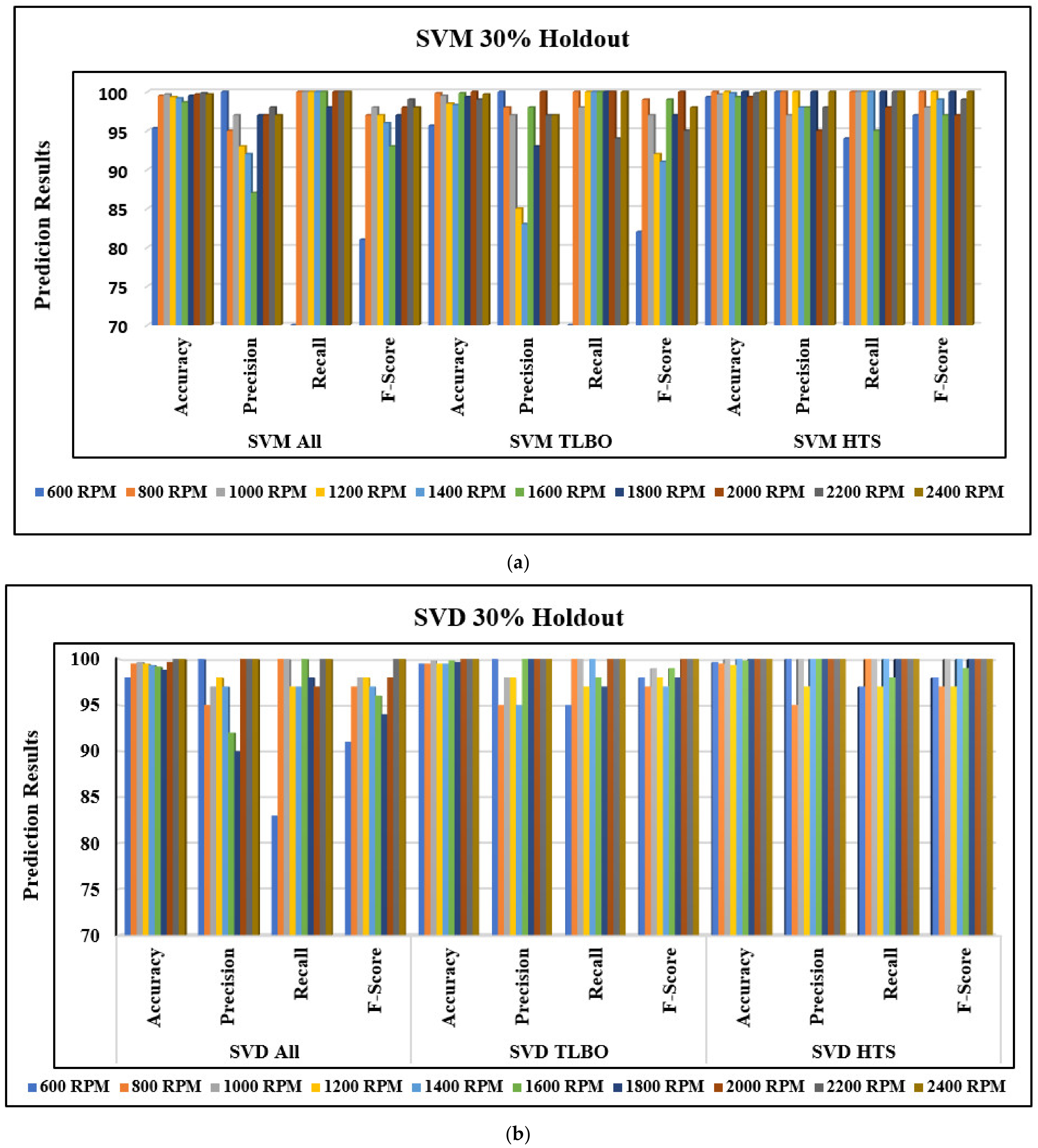
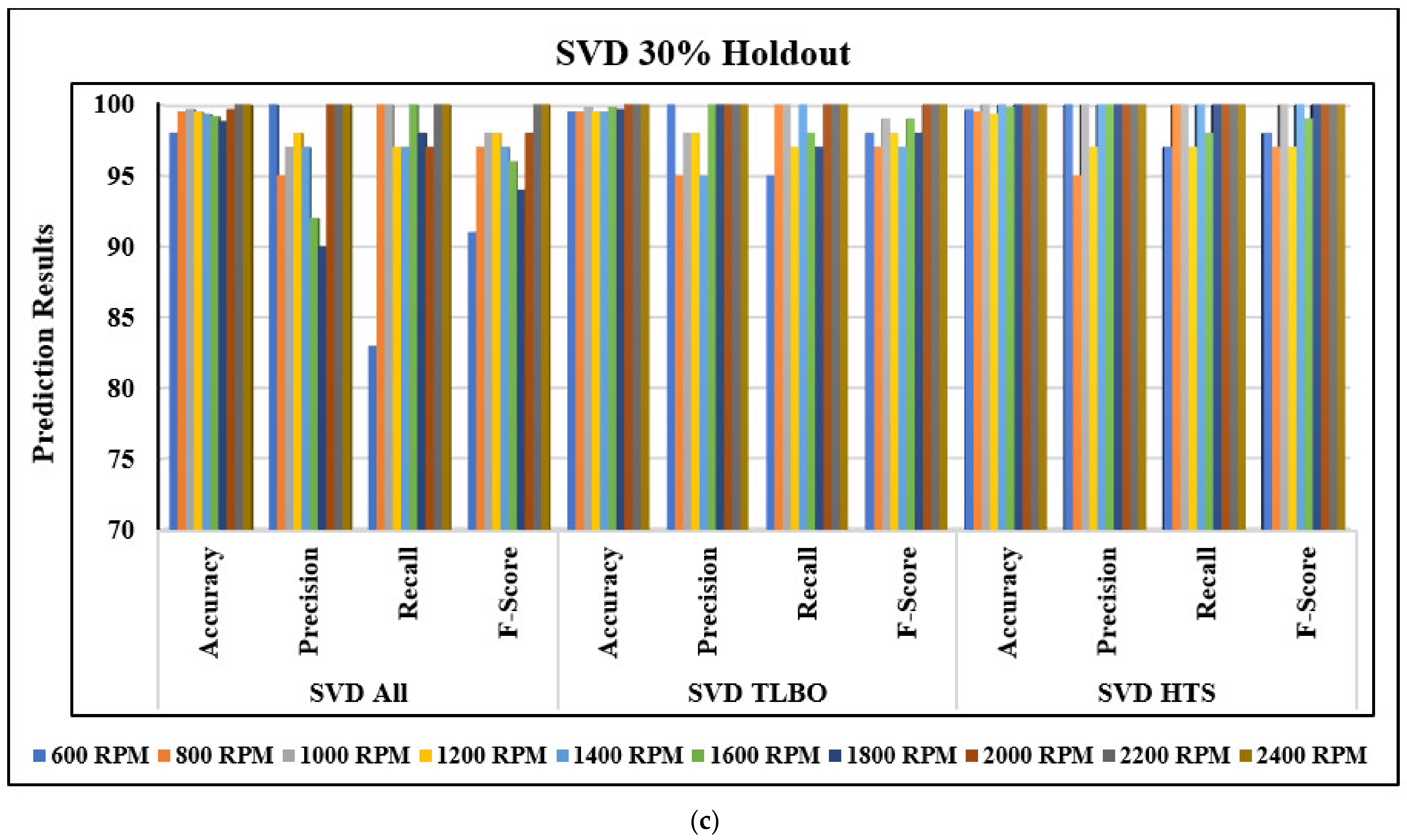
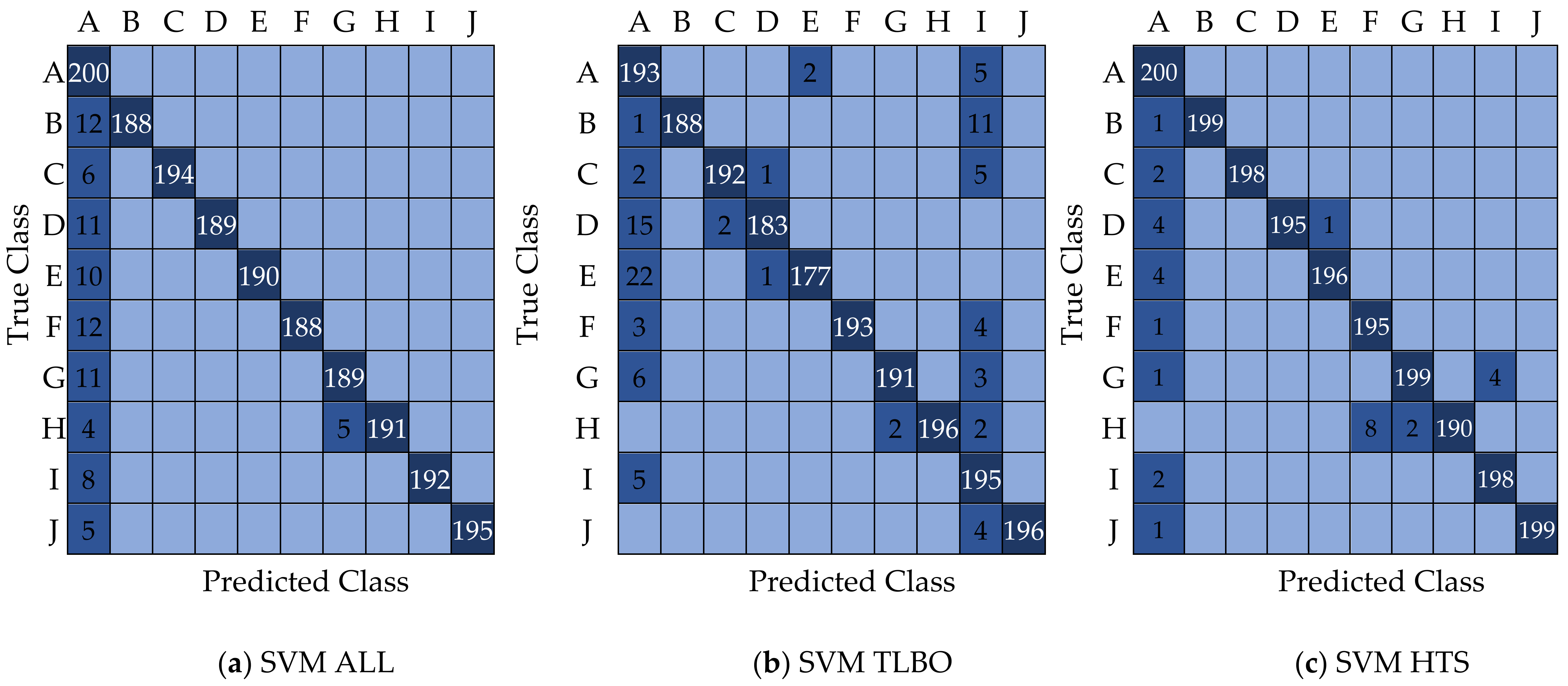
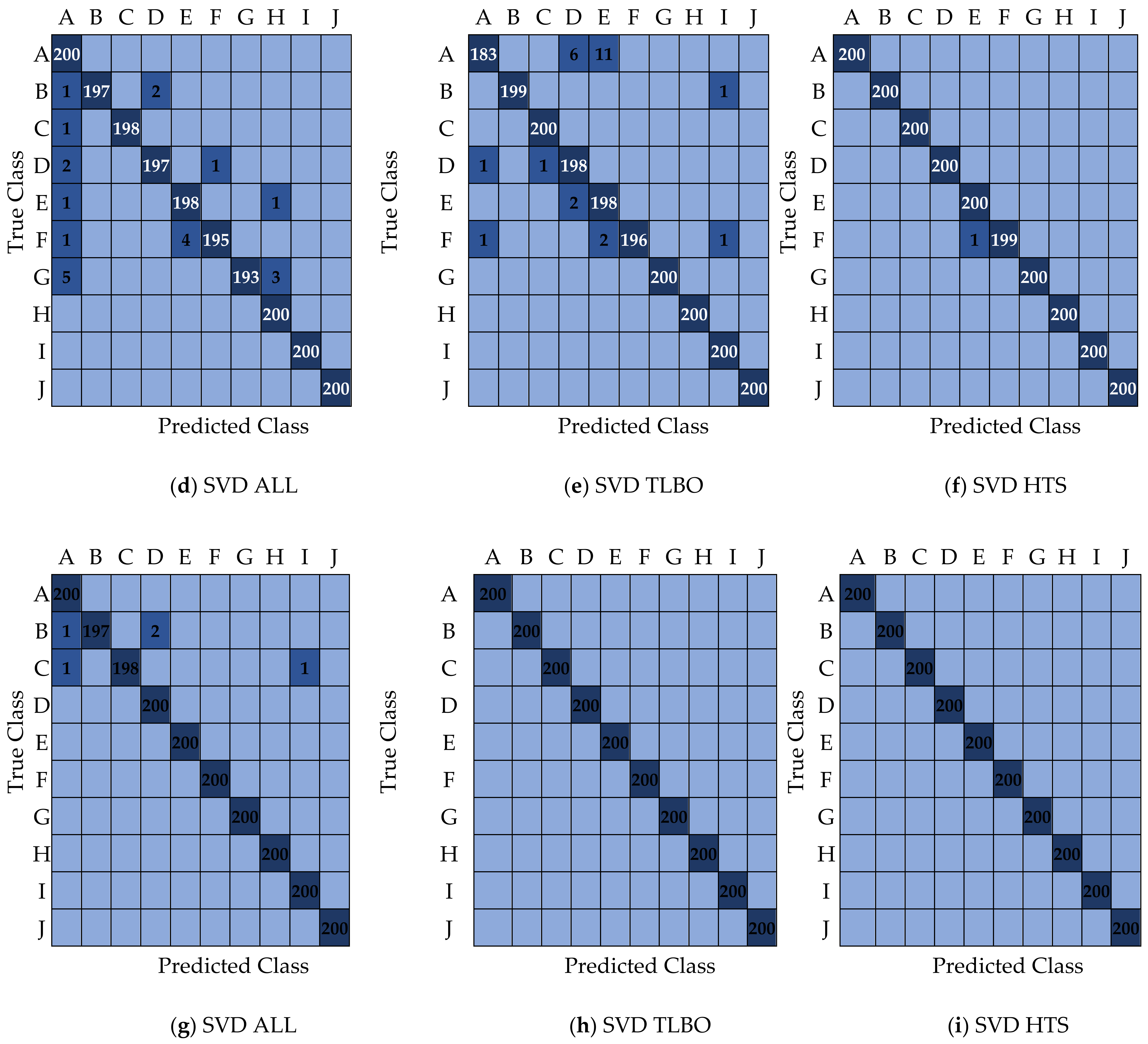
• Considering all IQP features with 30% hold-out testing, the maximum average accuracy to detect compound faults is observed as 99.8% with the ELM model.
• ELM-HTS and ELM-TLBO detect 100% compound faults with 30% hold-out testing, whereas the least average accuracy to detect compound faults is observed as 98.96% with SVM-TLBO.
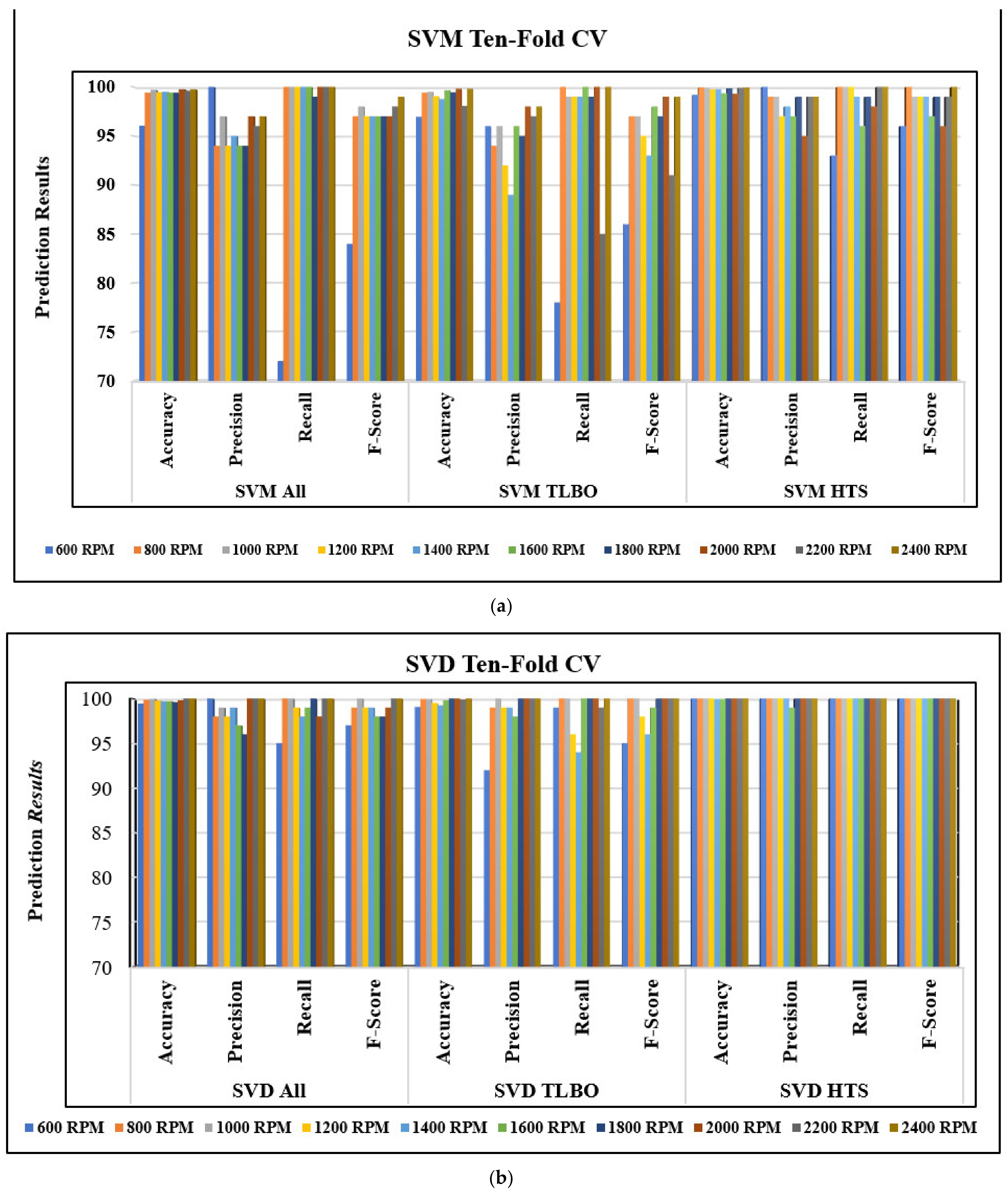
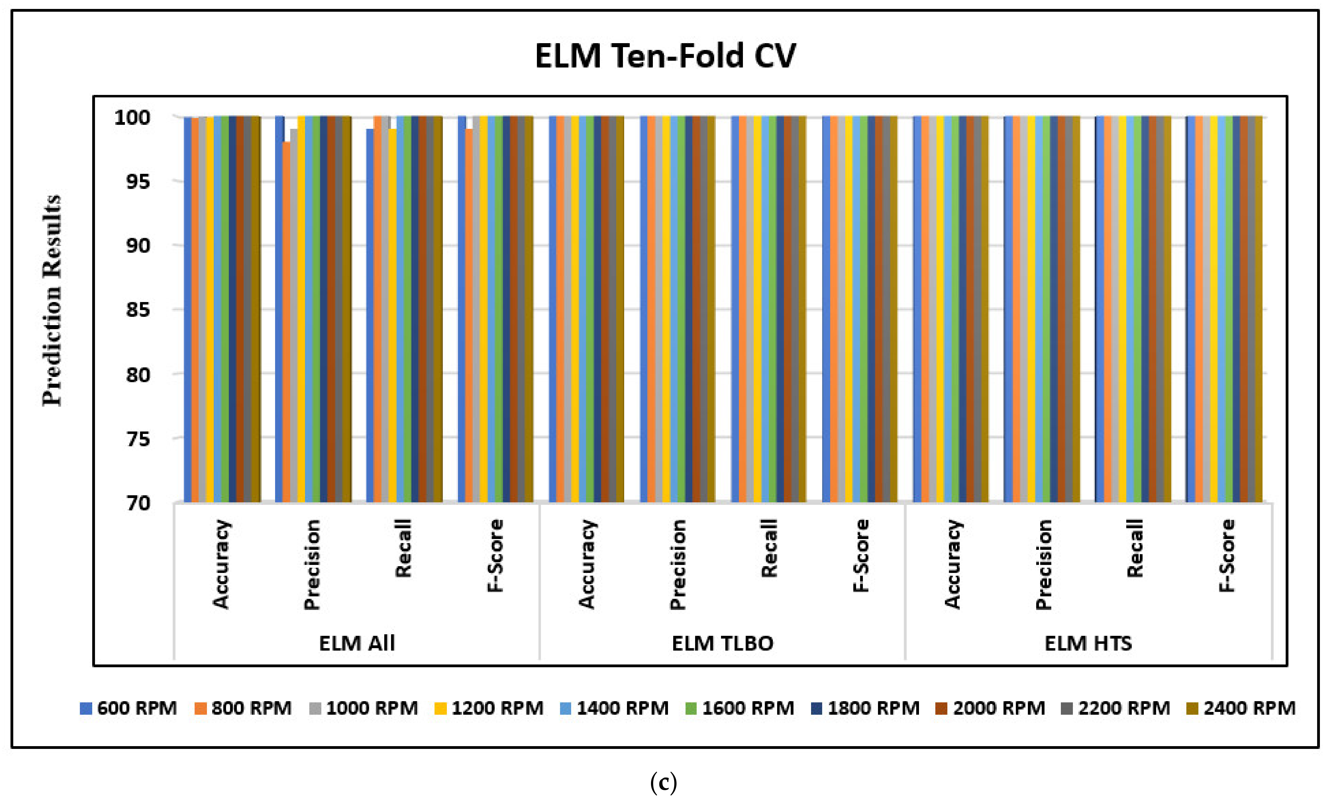
• With Ten-Fold CV and considering all IQP features, the maximum average accuracy to detect compound faults in REBs is reported as 99.9% with the ELM model.
• The maximum average compound fault detection accuracy of 100% is observed with ELM-HTS and ELM-TLBO. In contrast, the minimum average accuracy of 99.04% is reported from the SVM-TLBO model with the Ten-fold CV procedure.

The proposed methodology is useful for precisely diagnosing the bearing’s faults. When the available experimental data are limited, the approach may also be used for defect identification and the health monitoring of turbines, gears, pumps, and so on. Further findings illustrate the effectiveness of metaheuristic feature-selection algorithms, such as HTS and TLBO, in effectively identifying the important features for defect detection. The automation of condition monitoring and problem detection in industries is expected to gain traction in the near future with the augmented data generated by Multiscale-SinGAN.

References

1. Wang, H.; Du, W. Multi-source information deep fusion for rolling bearing fault diagnosis based on deep residual convolution neural network. Proc. Inst. Mech. Eng. Part C J. Mech. Eng. Sci. 2022, 236, 7576–7589. [Google Scholar] [CrossRef]
2. Glowacz, A. Fault diagnosis of single-phase induction motor based on acoustic signals. Mech. Syst. Signal Process. 2019, 117, 65–80. [Google Scholar] [CrossRef]
3. Venkatesh, S.; Sugumaran, V. A combined approach of convolutional neural networks and machine learning for visual fault classification in photovoltaic modules. Proc. Inst. Mech. Eng. Part O J. Risk Reliab. 2021, 236, 148–159. [Google Scholar] [CrossRef]
4. Cascales-Fulgencio, D.; Quiles-Cucarella, E.; García-Moreno, E. Computation and Statistical Analysis of Bearings’ Time- and Frequency-Domain Features Enhanced Using Cepstrum Pre-Whitening: A ML- and DL-Based Classification. Appl. Sci. 2022, 12, 10882. [Google Scholar] [CrossRef]
5. Vakharia, V.; Gupta, V.; Kankar, P. Nonlinear dynamic analysis of ball bearings due to varying number of balls and centrifugal force. In Mechanisms and Machine Science, Proceedings of the 9th IFToMM International Conference on Rotor Dynamics, Milan, Italy, 22–25 September 2014; Springer: Cham, Switzerland, 2015; pp. 1831–1840. [Google Scholar] [CrossRef]
6. Zhang, Y.; Ren, G.; Wu, D.; Wang, H. Rolling Bearing Fault Diagnosis Utilizing Variational Mode Decomposition Based Fractal Dimension Estimation Method. Measurement 2021, 181, 109614. [Google Scholar] [CrossRef]
7. Gu, J.; Peng, Y. An Improved Complementary Ensemble Empirical Mode Decomposition Method and Its Application in Rolling Bearing Fault Diagnosis. Digit. Signal Process. 2021, 113, 103050. [Google Scholar] [CrossRef]
8. Duan, R.; Liao, Y.; Yang, L.; Xue, J.; Tang, M. Minimum Entropy Morphological Deconvolution and Its Application in Bearing Fault Diagnosis. Measurement 2021, 182, 109649. [Google Scholar] [CrossRef]
9. Anbu, S.; Thangavelu, A.; Ashok, S.D. Fuzzy C-Means Based Clustering and Rule Formation Approach for Classification of Bearing Faults Using Discrete Wavelet Transform. Computation 2019, 7, 54. [Google Scholar] [CrossRef] [Green Version]
10. Gelman, L.; Persin, G. Novel Fault Diagnosis of Bearings and Gearboxes Based on Simultaneous Processing of Spectral Kurtoses. Appl. Sci. 2022, 12, 9970. [Google Scholar] [CrossRef]
11. Bhupendra, M.K.; Miglani, A.; Kumar Kankar, P. Deep CNN-based damage classification of milled rice grains using a high-magnification image dataset. Comput. Electron. Agric. 2022, 195, 106811. [Google Scholar] [CrossRef]
12. Vakharia, V.; Gupta, V.; Kankar, P. A multiscale permutation entropy-based approach to select wavelet for fault diagnosis of ball bearings. J. Vib. Control 2014, 21, 3123–3131. [Google Scholar] [CrossRef]
13. Pan, T.; Chen, J.; Zhang, T.; Liu, S.; He, S.; Lv, H. Generative adversarial network in mechanical fault diagnosis under small sample: A systematic review on applications and future perspectives. ISA Trans. 2021, 128, 1–10. [Google Scholar] [CrossRef] [PubMed]
14. Guo, X.; Liu, X.; Królczyk, G.; Sulowicz, M.; Glowacz, A.; Gardoni, P.; Li, Z. Damage Detection for Conveyor Belt Surface Based on Conditional Cycle Generative Adversarial Network. Sensors 2022, 22, 3485. [Google Scholar] [CrossRef] [PubMed]
15. Goodfellow, I.; Pouget-Abadie, J.; Mirza, M.; Xu, B.; Warde-Farley, D.; Ozair, S.; Courville, A.; Bengio, Y. Generative adversarial nets. Adv. Neural Inf. Process. Syst. 2014, 27, 2672–2680. [Google Scholar] [CrossRef]
16. Gao, S.; Wang, X.; Miao, X.; Su, C.; Li, Y. ASM1D-GAN: An Intelligent Fault Diagnosis Method Based on Assembled 1D Convolutional Neural Network and Generative Adversarial Networks. J. Signal Process. Syst. 2019, 91, 1237–1247. [Google Scholar] [CrossRef]
17. Lee, Y.O.; Jo, J.; Hwang, J. Application of deep neural network and generative adversarial network to industrial maintenance: A case study of induction motor fault detection. In Proceedings of the2017 IEEE International Conference on Big Data (Big Data), Boston, MA, USA, 11–14 December 2017; pp. 3248–3253. [Google Scholar] [CrossRef]
18. Shah, M.; Vakharia, V.; Chaudhari, R.; Vora, J.; Pimenov, D.Y.; Giasin, K. Tool wear prediction in face milling of stainless steel using singular generative adversarial network and LSTM deep learning models. Int. J. Adv. Manuf. Technol. 2022, 121, 723–736. [Google Scholar] [CrossRef]
19. Tubishat, M.; Ja’afar, S.; Alswaitti, M.; Mirjalili, S.; Idris, N.; Ismail, M.A.; Omar, M.S. Dynamic Salp Swarm Algorithm for Feature Selection. Expert Syst. Appl. 2021, 164, 113873. [Google Scholar] [CrossRef]
20. Dave, V.; Singh, S.; Vakharia, V. Diagnosis of Bearing Faults Using Multi Fusion Signal Processing Techniques and Mutual Information. Indian J. Eng. Mater. Sci. 2020, 27, 878–888. [Google Scholar]
21. Li, B.; Zhang, P.; Liang, S.; Ren, G. Feature extraction and selection for fault diagnosis of gear using wavelet entropy and mutual information. In Proceedings of the 2008 9th International Conference on Signal Processing, Beijing, China, 26–29 October 2008; pp. 2846–2850. [Google Scholar] [CrossRef]
22. Shen, J.; Xu, F. Method of fault feature selection and fusion based on poll mode and optimized weighted KPCA for bearings. Measurement 2022, 194, 110950. [Google Scholar] [CrossRef]
23. Huang, N.; Wu, Z. A review on Hilbert-Huang transform: Method and its applications to geophysical studies. Rev. Geophys. 2008, 46, 1–23. [Google Scholar] [CrossRef] [Green Version]
24. Shaham, T.R.; Dekel, T.; Michaeli, T. Singan: Learning a generative model from a single natural image. In Proceedings of the IEEE/CVF International Conference on Computer Vision, Seoul, Republic of Korea, 27 October–2 November 2019; pp. 4570–4580. [Google Scholar] [CrossRef]
25. Rao, R.; Savsani, V.; Vakharia, D. Teaching–Learning-Based Optimization: An optimization method for continuous non-linear large-scale problems. Inf. Sci. 2012, 183, 1–15. [Google Scholar] [CrossRef]
26. Rao, R.; Patel, V. An elitist teaching-learning-based optimization algorithm for solving complex constrained optimization problems. Int. J. Ind. Eng. Comput. 2012, 3, 535–560. [Google Scholar] [CrossRef]
27. Patel, V.; Savsani, V. Heat transfer search (HTS): A novel optimization algorithm. Inf. Sci. 2015, 324, 217–246. [Google Scholar] [CrossRef]
28. Cortes, C.; Vapnik, V. Support-vector networks. Mach. Learn. 1995, 20, 273–297. [Google Scholar] [CrossRef]
29. Vakharia, V.; Gupta, V.K.; Kankar, P.K. A comparison of feature ranking techniques for fault diagnosis of ball bearing. Soft Comput. 2016, 20, 1601–1619. [Google Scholar] [CrossRef]
30. Huang, G.; Wang, D.; Lan, Y. Extreme learning machines: A survey. Int. J. Mach. Learn. Cybern. 2011, 2, 107–122. [Google Scholar] [CrossRef]
31. Sharma, N.; Deo, R. Wind speed forecasting in Nepal using self-organizing map-based online sequential extreme learning machine. Predict. Model. Energy Manag. Power Syst. Eng. 2021, 1, 437–484. [Google Scholar] [CrossRef]
32. Malik, H.; Fatema, N.; Iqbal, A. Intelligent Data Analytics for Power Quality Disturbance Diagnosis Using Extreme Learning Machine (ELM). In Intelligent Data-Analytics for Condition Monitoring; Academic Press: Cambridge, MA, USA; pp. 91–114. [CrossRef]
33. Elen, A.; Avuçlu, E. Standardized Variable Distances: A distance-based machine learning method. Appl. Soft Comput. 2021, 98, 106855. [Google Scholar] [CrossRef]
Figure 1. Flowchart of methodology.
Machines 11 00029 g001
Figure 2. The architecture of single natural image Generative Adversarial Networks.
Machines 11 00029 g002
Figure 3. Pseudocode of the TLBO algorithm.
Machines 11 00029 g003
Figure 4. Pseudocode of the HTS algorithm.
Machines 11 00029 g004
Figure 5. Architecture of Extreme Learning Machine.
Machines 11 00029 g005
Figure 6. Classification with SVD.
Machines 11 00029 g006
Figure 7. Machinery Fault Simulator Setup.
Machines 11 00029 g007
Figure 8. Bearing with compound fault.
Machines 11 00029 g008
Figure 9. (ad) FFT plot at (a) 800 rpm, (b) 1400 rpm, (c) 1800 rpm, and (d) 2200 rpm.
Machines 11 00029 g009aMachines 11 00029 g009b
Figure 10. Kurtogram generation using SinGAN at various scales.
Machines 11 00029 g010aMachines 11 00029 g010b
Figure 11. (ac) Compound fault prediction: (a) SVM (b) SVD, and (c) ELM ML models at 30% hold-out.
Machines 11 00029 g011aMachines 11 00029 g011b
Figure 12. (ac) Compound fault prediction: (a) SVM (b) SVD, and (c) ELM models with ten-fold CV.
Machines 11 00029 g012aMachines 11 00029 g012b
Figure 13. (ai) Confusion matrix from Ten-fold CV with SVM, SVD, and ELM ML models.
Machines 11 00029 g013aMachines 11 00029 g013b