Tool Wear Monitoring Based on the Gray Wolf Optimized Variational Mode Decomposition Algorithm and Hilbert–Huang Transformation in Machining Stainless Steel

Abstract

The online monitoring and prediction of tool wear are important to maintain the stability of machining processes. In most cases, the tool wear condition can be evaluated by signals such as force, sound, vibration, and temperature, which are often processed via Fourier-transform based methods, typically, the short-time Fourier transform (STFT). However, the fixed-width window function in STFT has many limitations. In this paper, a novel tool wear monitoring method based on variational mode decomposition (VMD) and Hilbert–Huang transformation (HHT) were developed to monitor the wear of carbide tools in machining stainless steel. In this method, the intrinsic mode function (IMF) was used as the fitness function, and the (K alpha) parameter sets for VMD were optimized by the gray wolf optimization (GWO). The results show that the characteristic frequency in the GWO-VMD-HHT method is more significant with no aliasing compared with the EMD-HHT method, and an obvious characteristic frequency shift phenomenon is present. By utilizing the energy value of IMF₃ as the feature to classify the wear state of the cutting tool, the increase of energy reached 85.48% when 260–315 milling passes were in severe wear state. GWO, which can accurately find the best parameters for VMD, not only solves the problem that the Entropy Function is not suitable for force signals, but also provides reference for the selection of parameters of VMD.

1. Introduction

In the cutting of hard-to-machine metals, such as Ti alloys and Ni-based superalloys, tool wear is severe due to the high temperature and severe abrasion at the tool/chip and tool/workpiece interfaces. Tool wear can cause high-surface roughness and poor-surface quality of the workpiece. Severely worn tools often cause increased cutting forces and significant vibrations of the cutting system. Excessive tool wear not only leads to unexpected tool failure, but also affects the reliability and quality of the end products. To avoid unexpected tool failure and serious accidents caused by tool wear, preemptive tool changes must be made before tool life is reached in the production processes, and only 50~80% of tool life is effectively used in industry practice [1]. This practice not only increases production costs, but also poses a substantial environmental burden in terms of the energy and materials required for tool production. Therefore, it is important to implement online monitoring on the wear conditions of cutting tools. The accurate monitoring of tool wear can contribute to optimal timing for tool replacements, increase the machining efficiency, and reduced costs.

Over the past decades, there was extensive research on tool wear and tool wear monitoring. Figure 1 shows tungsten steel tools with different coatings for different purposes. It was proven that the wear of cutting tools is affected by many factors, and different wear mechanisms exist when the machining conditions are different. In high-speed milling processes, the cutting is interrupted, and the cutting frequency is higher, hence, tool wear is accelerated. Li et al. [2] used cutting fluid with graphene oxide suspension in the high speed drilling of Ti6Al4V, and found that the cutting force was significantly reduced by 17.21% due to the reduction of friction wear. In investigating the machinability of a titanium matrix composite (TMC), they found that the agglomeration of carbon nanotubes (CNTs) and the presence of titanium carbide (TiC) particles formed in situ in the titanium matrix caused sever tool wear [3]. For the advanced tools, such as polycrystalline diamond (PCD), adhesive–abrasive were the dominant wear mechanism [4]; residual stress and graphitization, which can cause fracture and dislodgement of diamond particles, also affects the development of tool wear [5]. These types of wear are difficult to predict, thus, it becomes necessary monitor the level of tool wear by developing and implementing appropriate methods.

Monitoring the wear of milling tools is a challenging task due to the nonlinear and time-varying characteristics of machining processes. This makes it difficult to establish a theoretical model for accurately monitoring. The monitoring of tool wear condition can be classified as direct monitoring and indirect monitoring. The indirect monitoring method does not interfere with normal cutting operations and is easier to carry out online. Compared with the direct monitoring method, it can better determine the tool wear condition and avoid the influence of cutting fluid and other factors. Cutting force [6,7,8,9], vibration [10,11,12] and acoustic emission [13,14,15] are the most commonly used signals in tool wear monitoring. With the continuous wearing of the tool, cutting forces generated in cutting operation may change, thus, the force signal, which reflects the wearing condition of the tool, is considered the most reliable approach to monitoring tool wear [16]. Bernini et al. [17] proposed a method for monitoring the wear of milling tools that were used under various lubrication conditions, and verified it on different machine tools. When the material experienced plastic deformation or fracture due to the cutting forces, the elastic forces and the cohesive forces of the crystals can be instantaneously released in the form of energy; acoustic emission signals are thus generated and can be detected by emission sensors that usually have strong anti-interference ability and high sensitivity. These sensors are easy to install with low cost, and have found wide applications in tool wear monitoring. Thirukkumaran et al. [18] studied the relationship between tool wear and wavelet coefficient with different tool geometries, and showed that wavelet packet transformation can distinguish the relevant damage mechanism during drilling by different frequency components. Vibration signals obtained in the milling processes can directly reflect the wear conditions. This is because the friction among the tool, workpiece, and chips leads to variations in the dynamic component of the force. However, vibration signals are prone to being affected by both machining system and environmental vibrations, which can result in lower monitoring accuracy and reliability compared to force signals. Delolmo et al. [19] proposed a monitoring method for high-speed broaching, and established the sensitivity between tool wear and the natural frequency of broaching. Thanks to the rapid development of neural networks and machine learning, tool life can be accurately predicted by analyzing the mapping relationship between signal features and tool wear. Gomes et al. [20] proposed a recursive feature elimination method to select the features of the input SVM AI model, and the classification accuracy reached 97.54%. In the area of short-term and long-term prediction of tool wear; Cheng et al. [21] proposed a tool state model based on dense residual neural networks, which has greater efficiency and robustness compared to other models. Liu et al. [22] incorporated duration and working mode into the proposed novel-switching, hidden, semi-Markov model, and successfully monitored tool wear under time-varying cutting conditions. Kotsiopoulos et al. [23] proposed a system to automate quality inspection and machine condition monitoring by investigating the defects on hard mental samples. Three different models were developed to analyze the microprofilometer data, the ultrasound data and the shop floor data, respectively, and the results show that the fusion model was significantly better in terms of recall, accuracy, F-score and precision. In their review, Papageorgiou et al. [24] pointed out that among the various AI techniques, deterministic methods are the most popular choice. However, despite the successful application of AI in Root Cause Analysis (RCA), there are still challenges that need to be addressed, e.g., interpretability, training quality, privacy and security.

The Fast Fourier transform (FFT) is the most widely used method in the frequency analysis of the cutting forces. However, this method lacks the capability to describe the frequency components of a signal at a certain time. In contrast, the time-frequency analysis has a good characterization capability for both the time and frequency domains, enabling the determination of local characteristics associated with tool wear state [25,26]. STFT solves the problem that FFT cannot analyze non-smooth signals. It can convert one-dimensional signals to two-dimensional signals [27]. Jauregui et al. [28] estimated the condition of tool wear in high-speed micromilling based on cutting force signals and vibration signals. The results showed that the main frequency changed due to tool wear. Zhou et al. [29] established a wavelet basis selection method and found that the mean value of holder exponents (HE) value and the singular number of vibration components in the feed direction have the highest correlation with the tool conditions. The empirical mode decomposition (EMD) [30] was used in many practical engineering applications [31,32,33] since the end of the 20th century. However, EMD is prone to endpoint effects in decomposing signals into IMFs, which in turn causes some IMF_s to lose their physical meaning. The Hilbert–Huang transform (HHT) can decompose the transient signals of nonlinear systems and are suitable for analyzing nonlinear and transient signals [34]. Susanto et al. [35] evaluated the machining stability via HHT, demonstrating its feasibility in the monitoring of the ever-changing state of the machining process. Yang et al. [36] proposed a filtering criterion based on the average energy percentage of the IMF components. The results showed that the application of HHT in the processing of acoustic emission signals had significant potential for monitoring grinding burn. Mahata et al. [37] proposed a monitoring method that extracts time-frequency domain features of signals by HHT and support vector machine to identify grinding wheel wear with 100% accuracy at both low- and high-cutting depths.

In 2013, variational mode decomposition (VMD) [38] was proposed. It is a collection of adaptive Wiener filter banks that convert signal decomposition issues into issues with variable decomposition. Compared to EMD, VMD has strong robustness and a solid mathematical theoretical foundation, but the number K of VMD modalities must be determined manually. The number of modes can interfere with the decomposition of the signal, which affects the recognition accuracy of useful information features. It is necessary to have some prior knowledge of the original signal in order to determine K value. However, capturing the internal information characteristics of a signal is often difficult. Additionally, the bandwidth for each modality acquired by VMD is determined by the penalty factor. The larger the penalty factor, the narrower the bandwidth will be. The implementation of VMD in engineering signal processing is somewhat hampered by the acceptable choice of algorithm parameters and the issue of inadequate or excessive decomposition in VMD. To solve this problem, Wei et al. [39] proposed an improved empirical variational mode decomposition (EVMD) method for processing ultrasonic echo signals from coal and rock interfaces. Based on their experimental results, the suitable VMD parameters were selected and the coal rock interface was identified effectively. Su et al. [40] presented a mold-level prediction approach based on the long short-term memory concept and the multi-mode decomposition method. Compared to other decomposition techniques such as EMD, VMD successfully avoids modal aliasing and boundary effects. Wei et al. [41] proposed a signal decomposition method based on Whitening Variational Mode Decomposition (WVMD), which makes each IMF independent of each other. However, in their method, the parameters of VMD are manually selected. Aiming at the difficult problem of online monitoring of wheel wear status, Wan et al. [42] proposed a method to find the optimal parameter combination of VMD through the whale optimization algorithm, but they did not accurately find the optimal parameter combination of VMD during the simulation signal validation process. Liu et al. [43] analyzed the signal decomposition results under different combinations of VMD parameters, and thus determined the optimal VMD parameters with some chance. Bazi et al. [44] used VMD to pre-process the raw signal and then used the IMF as data for deep learning, but again they artificially determined the combination of parameters for the VMD. In addition, gray wolf optimization (GWO), a novel heuristic algorithm for solving optimization problems, was proposed by Mirjalili [45]. Shi et al. [46] proposed a method for accurately extracting wind turbine signal features by optimizing variational mode decomposition. In their method, the two parameters of VMD are independently selected, ignoring the relationship between the two parameters. Yan et al. [47] proposed a genetic algorithm to search for the optimal parameter combination of VMD, but their fitness function ignored the connection between IMF and the original signal. As such, the construction of the VMD parameter optimization objective function can directly affect the accuracy and efficiency of the final decomposition.

Based on the above introduction, it is clear that, for the vibration signal of rotating machinery, most of the fitness functions in the parameter optimization of VMD are permutation entropy, information entropy, etc. It is not feasible to use entropy as a fitness function for tool wear force signals. In this research, a tool wear monitoring method based on GWO-optimized VMD parameters is proposed. The energy difference between IMFs of the properly decomposed signal and the original signal was used as the fitness function, and the optimal combination of decomposition parameters for VMD was determined using GWO. Thus, modal mixing can be avoided under the condition of the best parameter combination. The energy of the IMF that exhibited the highest correlation with the original signal was selected as the feature to identify the wear state of the tool and accurately estimate the health of the tool.

2. Materials and Methods

In this section, the flow of the proposed method, the mathematical theory and its formula, as well as the experimental setup and corresponding experimental parameters are introduced.

2.1. Methods

Generally, time domain features such as mean, standard deviation, root mean square can be used for tool wear prediction. However, the recognition results based on the above features are not very reliable. VMD is a novel signal decomposition method that facilitates the extraction of useful information about tool wear.

2.1.1. Theoretical Foundations of VMD

VMD has the firm mathematical theoretical foundation compared to other signal decomposition methods, and its essence is Wiener filter. Decompose the original signal into a specified number of IMFs, and the process of VMD decomposing the signal can be described as [38]:

$$\underset{\{{\omega }_k\},\{{\omega }_k\}}{min}\{{\sum }_{k=1}^K\parallel {\partial }_t[(\delta (t)+\frac{j}{\pi t})\ast u_k(t)]e^{-j{\omega }_{k}t}{\parallel }_2^2\},$$

(1)

$$s.t.{\sum }_{k=1}^K{u}_k(t)=f(t),$$

(2)

where K is the number of IMF decompositions specified for the original signal, u_(k) is the Kth IMF component, and ω_k is the center frequency of the Kth IMF component, δ is the Dirac distribution. To solve Equation (1), the quadratic penalty term α and Lagrange multiplier λ were applied to make the problem unconstrained, the VMD variational problem can be denoted as follows:

$$L(\{u_k\},\{{\omega }_k\},\mathsf{\lambda })=\alpha {\displaystyle \sum }_{k=1}^K||{\partial }_t[({\delta }_t+\frac{j}{\pi t})\ast u_k(t)]e^{-j{\omega }_{k}t}|{|}^2+{||f(t)-{\displaystyle \sum }_{k=1}^K{u}_k||}_2^2+<\lambda (t),f(t)-{\displaystyle \sum }_{k=1}^K{u}_k(t)>$$

(3)

Equation (3) can be solved using the alternating direction method of the multiplier (ADMM). In addition, to update the mode and center frequency, the optimization problem can be solved according to the Parseval/Plancherel theorem. The specific steps for VMD are as follows:

(1) First, initialize ${\widehat{u}}_k^1$, ${\omega }_k^1$ and ${\widehat{\lambda }}^1$, and set the initial iteration number n to 0.

(2) Iteration n = n + 1.

(3) For k = 1:K, ${\widehat{u}}_k$ is updated for all ω ≥ 0.

$${\widehat{\omega }}_k^{n+1}(\omega )=\frac{\widehat{f}(\omega )-{\sum }_{i<k}{\widehat{u}}_i^{n+1}(\omega )-{\sum }_{i>k}{\widehat{u}}_i^n(\omega )+\frac{{\widehat{\lambda }}^n(\omega )}{2}}{1+2\alpha {(\omega -{\omega }_k^n)}^2}$$

(4)

Update ω_k:

$${\omega }_k^{n+1}=\frac{{\int }_0^{\infty }\omega {|{\hat{u}}_k^{n+1}(\omega )|}^{2}d\omega }{{\int }_0^{\infty }{|{\hat{u}}_k^{n+1}(\omega )|}^{2}d\omega }$$

(5)

where $\widehat{f}(\omega )$, ${\widehat{u}}_k^{n+1}(\omega )$ and ${\widehat{\lambda }}_k^{n+1}(\omega )$ are the Fourier transform of $f(t)$, $u_k^{n+1}(t)$ and ${\lambda }_k^{n+1}(t)$, respectively.

(4) Update λ

$${\widehat{\lambda }}^{n+1}(\omega )={\widehat{\lambda }}^n(\omega )+\tau (\widehat{f}(\omega )-{\displaystyle \sum }_k{\widehat{u}}_k^{n+1}(\omega ))$$

(6)

where τ is an update parameter, which is usually set to 0.

(5) Repeat steps (3)~(5) until the iteration termination conditions are met:

$${{\displaystyle \sum }}_k(||{\widehat{u}}_k^{n+1}-{\widehat{u}}_k^n|{|}^2/||\widehat{u_k^n}|{|}^2)<\epsilon$$

(7)

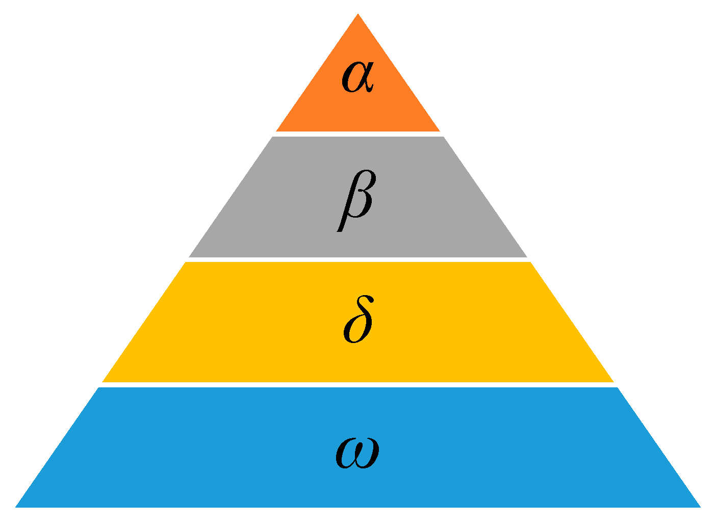
2.1.2. VMD Parameter Selection Based on Grey Wolf Optimization Algorithm

Grey wolves’ hunting mechanism is simulated by the grey wolf optimization algorithm based on their social characteristics. There is a strict pyramid hierarchy within the wolf in Figure 2. The three levels of wolf α, β, and δ correspond to the three solutions with the best adaptability. The entire hunting process was guided by α, β, and δ wolves. The first layer of gray wolves is the head wolf α, which is in the leadership position of the wolf pack. The second layer of wolves is β wolf, which assists α wolves in leading hunting and other behaviors and is a replacement after the death of α wolves. The third layer of wolves is the lowest δ wolves in leadership; the majority of the pack are grassroot ω wolves who surround their prey.

In each iteration, all wolves, led by the leader, more deeply explore into the space where the prey is most likely to be present. The formula for encircling prey can be expressed as:

$$\overrightarrow{D}=|\overrightarrow{C}\cdot {\overrightarrow{X}}_p(t)-\overrightarrow{X}(t)|$$

(8)

$$\overrightarrow{X}(t+1)={\overrightarrow{X}}_p(t)-\overrightarrow{A}\cdot \overrightarrow{D}$$

(9)

where t denotes the current number of iterations, ${\overrightarrow{X}}_p(t)$ indicates the current position vector of the prey, $\overrightarrow{X}(t)$ is the position vector of the gray wolf, and $\overrightarrow{A },\overrightarrow{C}$ are the synergistic coefficient vectors, and the calculation formula is as follows:

$$\overrightarrow{A}=2\overrightarrow{a}\cdot {\overrightarrow{r}}_1-\overrightarrow{a}$$

(10)

$$\overrightarrow{C}=2\cdot {\overrightarrow{r}}_2$$

(11)

During iteration, the convergence factor $\overrightarrow{a}$ decreases linearly in the interval [2, 0], and ${\overrightarrow{r}}_1$, ${\overrightarrow{r}}_2$ are random vectors in the interval [2, 0].

In the process of iteration, the optimal values of the objective function are selected by the α, β, δ wolves in turn, and guide the grassroot ω wolves to surround their prey, the process can be expressed as:

$$\begin{gathered} {\overrightarrow{D}}_{\alpha }=|{\overrightarrow{D}}_1\cdot {\overrightarrow{X}}_{\alpha }-\overrightarrow{X}| \\ {\overrightarrow{D}}_{\beta }=|{\overrightarrow{D}}_2\cdot {\overrightarrow{X}}_{\beta }-\overrightarrow{X}| \\ {\overrightarrow{D}}_{\delta }=|{\overrightarrow{D}}_3\cdot {\overrightarrow{X}}_{\delta }-\overrightarrow{X}| \\ {\overrightarrow{X}}_1={\overrightarrow{X}}_{\alpha }-{\overrightarrow{A}}_1\cdot ({\overrightarrow{D}}_{\alpha }) \\ {\overrightarrow{X}}_2={\overrightarrow{X}}_{\beta }-{\overrightarrow{A}}_2\cdot ({\overrightarrow{D}}_{\beta }) \\ {\overrightarrow{X}}_3={\overrightarrow{X}}_{\delta }-{\overrightarrow{A}}_3\cdot ({\overrightarrow{D}}_{\delta }) \\ \overrightarrow{X}(t+1)=\frac{{\overrightarrow{X}}_1+{\overrightarrow{X}}_2+{\overrightarrow{X}}_3}{3} \end{gathered}$$

(12)

where $D_{\alpha }$, $D_{\beta }$, $D_{\delta }$ is the distance between the optimal three wolves and their prey, $X_{\alpha }$, $X_{\beta }$, $X_{\delta }$ are the position vectors of the optimal three wolves, and $\overrightarrow{X}(t+1)$ is the position of the updated ω wolf according to the position of the optimal three wolves.

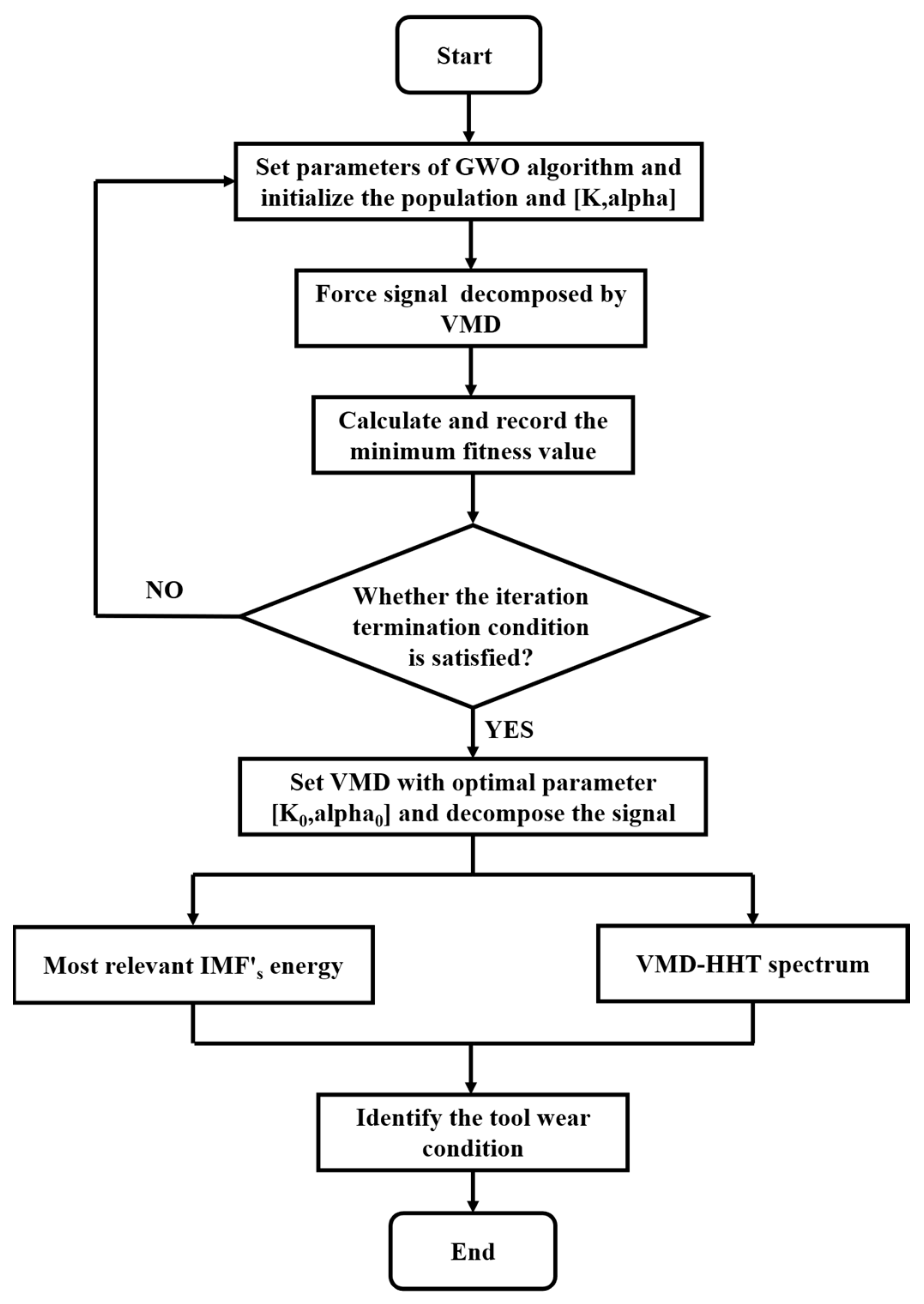
2.1.3. GWO Optimizes the VMD Parameter Flow

The key to VMD parameter optimization using GWO algorithm optimization is to select the appropriate fitness function, and the entire wolf packs iteratively update the position according to the fitness function to find the minimum fitness value. The combination of (K, alpha) without under-decomposition and over-decomposition is the ideal VMD parameter after VMD processing. If the original signal is correctly decomposed by the VMD, the total energy of each IMF should be equal to the total energy of the original signal. The above can be described as:

$$\begin{gathered} E_{Original}=\sqrt{\frac{{\sum }_{i=1}^n{x}_i^2}{n}} \\ {E}_{IM{F}_s}=E_1+E_2+···+E_n \\ \Delta E=E_{Original}-E_{IM{F}_s} \end{gathered}$$

(13)

where E_Original is the energy of the original signal, E_IMFs is the total energy of the IMFs, ∆E is the energy difference.

The steps for adapting VMD parameters based on the GWO algorithm are shown below:

(1) Initialize the VMD parameter optimization interval. where K ranges from [2, 9] and alpha in the range [1000, 7000].

(2) Both the population number of gray wolves and the maximum number of iterations are set to 20.

(3) According to the position of the wolf pack, the fitness function value was calculated, and the three wolves with the largest fitness function value were used as α, β, δ wolves in turn.

(4) Update the position of the gray wolf according to Equation (9).

(5) Repeat steps (3) and (4) until the maximum number of iterations was reached.

The process of the tool wear monitoring method based on GWO-optimized VMD parameters is as follows. Firstly, the fitness function is determined by calculating the energy difference between the original signal and the total IMFs. Secondly, the optimal parameters of the VMD are searched for by the GWO algorithm. Then, VMD decomposes the original force signal; the correlation coefficient is applied to identify the IMF that exhibits the highest correlation with the original signal. Finally, the energy of the IMF most correlated with the original signal and the VMD-HHT Spectrum is used to recognize the tool wear condition. The flowchart of the entire monitoring method is shown in Figure 3.

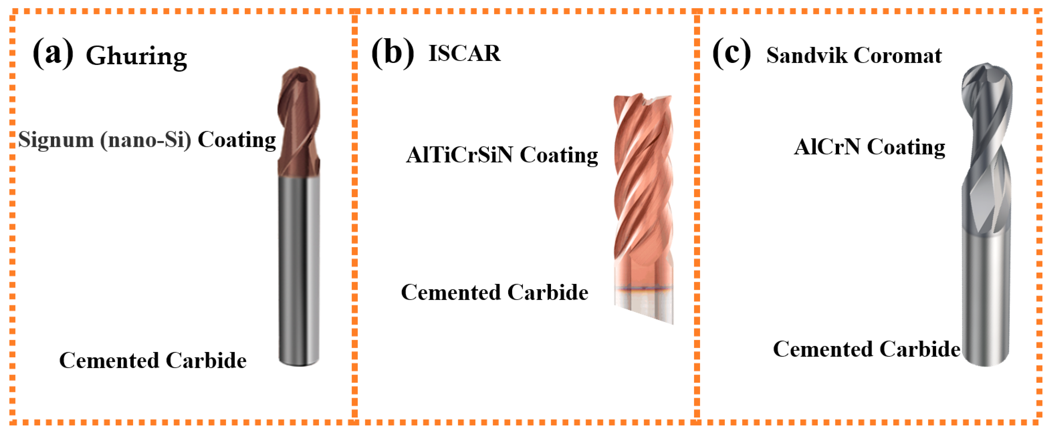
2.2. Materials and Experimental Description

To evaluate the above proposed method, a public data set from the 2010 PHM competition was used for validation [48]. As shown in Figure 4, the cutting force signals were recorded by a quartz 3-axis dynamometer (Kistler 9265B, Kistler Group, Eulachstrasse 22, 8408 Winterthur, Switzerland), and were converted into voltage signals via a multichannel charge amplifier (Kistler 5019A, Kistler Group, Eulachstrasse 22, 8408 Winterthur, Switzerland). The flank wear of three flutes was measured by LEICA MZ12 microscope at the end of each pass. This resulted in a total of 6 data sets (C1, C2, …, C6), each of which corresponds to 315 milling passes of the corresponding milling cutter. The signal data collected for each milling process includes high-frequency milling force and vibration signals in the 3 axes, as well as high-frequency acoustic emission signals. All signals were acquired by the NI DAQ PCI 1200 at a 50 kHz sampling rate, and the processing parameters are shown in

Table 1. Experiment parameters of PHM2010.

Spindle Speed (r/min)	Feed Rate (mm/min)	Radial Cutting Depth (mm)	Axial Cutting Depth (mm)	Sampling Rate (kHz)
10,400	1555	0.125	0.2	50

.

3. Results

Before decomposing the actual force signal, it is necessary to construct a simulation signal to verify whether the proposed method can correctly find the best parameters of VMD, so we designed the following simulation signal.

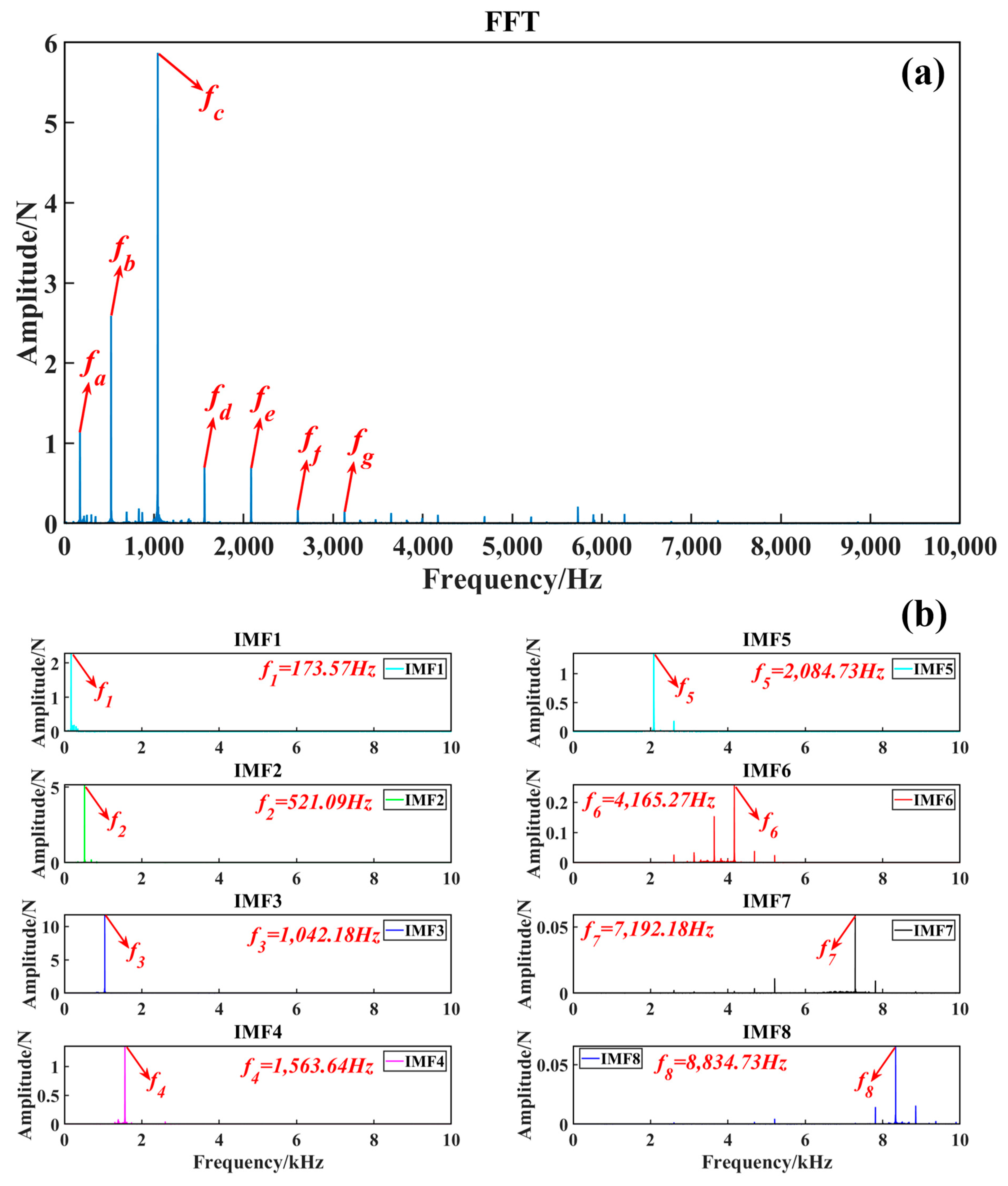
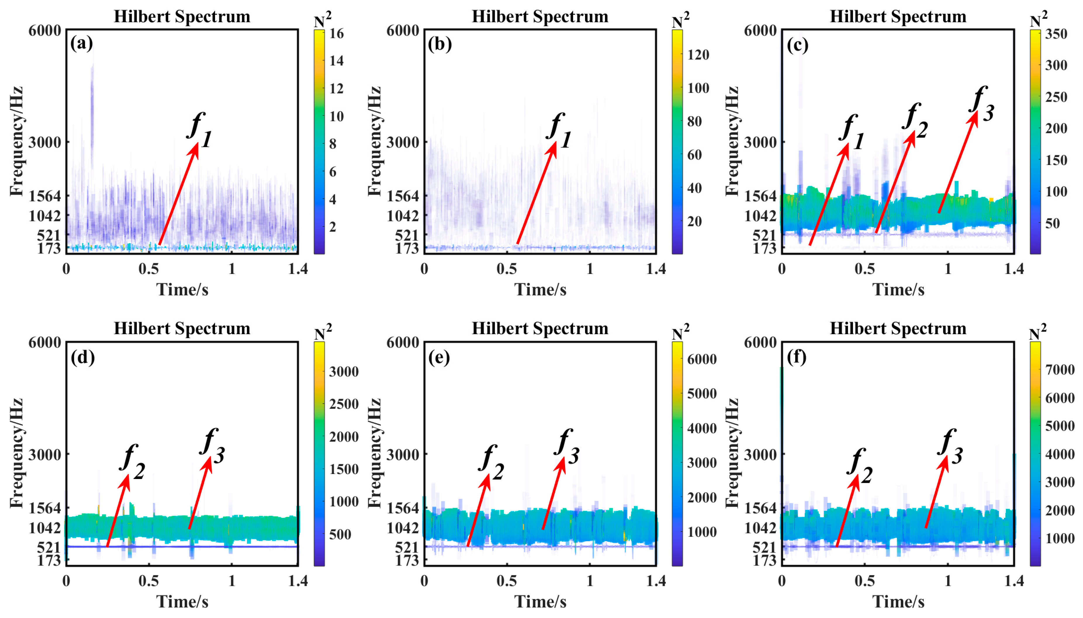
3.1. Simulation Signal Analysis

The simulation signal was constructed: 50 Hz sine f₁(t) with an amplitude of 0.7, 120 Hz sine f₂(t) with an amplitude of 3, 300 Hz cosine f₃(t) with an amplitude of 2, and 200 Hz cosine f₄(t) with an amplitude of 4. White noise was denoted as n(t) with the mean of 0 and variance of 4 was added, and the signal was sampled at a rate of 1000 Hz, with a total sampling time of 1.5 s. The simulation signal is shown in Figure 5.

$$\{\begin{array}{l}f(t)=f_1(t)+f_2(t)+f_1(t)+f_4(t)+f_4(t)+n(t)\\ f_1(t)=0.7\cdot \sin (2\pi \cdot 50t)\\ f_2(t)=3\cdot \sin (2\pi \cdot 120t)\\ f_3(t)=2\cdot \cos (2\pi \cdot 300t)\\ f_4(t)=4\cdot \cos (2\pi \cdot 200t)\end{array}$$

(14)

Both the number of gray wolves and iterations are set to 20, and the optimal (K, alpha) combination is found through the iterative update of the algorithm. Figure 6 shows that the iterative convergence curve of the whole GWO algorithm. It can be seen from the curve that it converges after 11 iterative updates, and the fitness value is 0.0023 and stabilizes at this value, and the corresponding gray wolf position is the best parameter combination (4, 1608). It is shown that the optimization algorithm has a strong global optimization capability, converges quickly and successfully finds the best parameters for searching for the optimal parameters of VMD.

Once the GWO algorithm identifies the best combination of parameters for the VMD, this optimal set of parameters is then inputted into the VMD algorithm. The results of the decomposed simulation signal are shown in Figure 7; the different colors represent the different IMFs obtained through the VMD decomposition. The VMD algorithm accurately decomposes the simulation signal into 4 IMFs, as set out in Equation (11), meanwhile the individual IMF components are independent of each other, and no modal confounding occurs.

3.2. Force Signal Analysis

According to the change in flank wear of C1, there are three different stages: the initial wear, the steady tool wear: Normal A, Normal B, and the severe wear. From the 1st to the 60th times, high tool surface roughness and tissue defects result in poor tool wear resistance and therefore faster wear during initial wear stage. The surface roughness of the tool decreases after the initial wear, the surface pressure is evenly distributed, the tool wear is stable at this stage and the amount of wear is proportional to time. In the steady wear, the 61st~150th and 151st~260th times are defined as Normal A and Normal B, respectively. As the tool approaches its service life, the surface roughness increases, leading to an increase in cutting temperature and accelerated tool wear. This stage corresponds to the 261st~315th times. The wear curves and division of tool C1 are shown in Figure 8; the division of the wear phase of tool C1 is shown in

Table 2. Classification of wear stages of the tool C1.

Wear State	Label	VB Value (μm)	Times
Initial wear	1	39.64~90.44	1~60
Steady wear	2	90.62~99.88	61~150
	3	100.14~138.42	151~260
Severe wear	4	138.82~165.17	261~315

.

To increase the efficiency of the GWO algorithm and avoid irrelevant signals in the signals collected at the beginning of milling, the data was streamlined and 70,000 groups of data between 70,000~140,000 were selected. Taking the X-axis force signal collected during the 150th machining as an example, the parameters (K, alpha) of VMD were optimized by GWO, and the convergence process curve of the GWO optimization algorithm was shown in Figure 9. It can be seen from the curve that after four iteration updates, it converges, and the fitness value is 7.48 and stabilizes at this value, and the corresponding gray wolf position is the best parameter combination (8, 3977).

The spectrogram of 150th milling X-axis force signal obtained by FFT is shown in Figure 10a. The frequencies f_a to f_g are 173 Hz, 521 Hz, 1042 Hz, 1564 Hz, 2084 Hz, 2605 Hz, and 3126 Hz, respectively. Input K = 8, alpha = 3977 into VMD, the modal components of the 150th milling X-axis force signal obtained by VMD is shown in Figure 10b. The center frequency of IMFs after signal decompose by the VMD is very intuitive, and no modal mixing occurred, which proves that (8, 3977) is the best parameter for VMD. According to the parameters of the milling, the calculation shows that the spindle frequency is f_s = n/60 = 173.33 Hz, which is related to the frequencies of the spindle (rotating speed) and cutting flutes (cutting frequency), and the flutes frequency f_t = 3f_s = 521 Hz, n represents the spindle speed (rpm). From Figure 10b, it is apparent that the center frequency f₁ of IMF₁ is 173.57 Hz, which is the spindle frequency. The center frequency f₂ of IMF₂ is 521 Hz, which is the flutes frequency. The tool wear information is mainly concentrated in the low-frequency phase, and the high-frequency phase is mainly ambient noise. The frequency characteristics of the force signal are a good indicator of tool wear in milling. During milling processes, the spindle frequency f₁ = 173.33 Hz and its corresponding harmonic frequency dominate in the low-frequency bands, which is consistent with previous results [26,49]. The correlation coefficients of each IMF in the VMD decomposed force signal results and the original signal were calculated in

Table 3. Correlation coefficients of IMFs with the original signal.

IMF	IMF1	IMF2	IMF3	IMF4	IMF5	IMF6	IMF7	IMF8
correlation coefficient	0.1775	0.3721	0.8992	0.1045	0.1075	0.0383	0.0118	0.0093

. The correlation coefficient value between IMF₃ and the original signal has almost reached 0.9, and the center frequency f₃ of IMF₃ is 1042 Hz, which is the second harmonic of the milling frequency.

The FFT results of the X-axis force signal for the 1st, 30th, 105th, 205th, 285th and 315th milling are shown in Figure 11. Note that the amplitude of the spindle rotation frequency and its multiplier in the FFT results of the force signal are correlated with different tool wear states. When the tool is slightly worn, the amplitude of the signal is very small. As the number of millings increases, the tool wear intensifies, and the amplitude of the signal increases. It can be seen that frequency f₃ is closely related to the wear of the tool, and the energy associated with its IMF can be employed as a distinguishing factor for assessing the tool wear state.

Milling is a very complex process, and unlike the FFT, HHT [50] achieves uniform high resolution over the entire frequency range. The results of HHT of the IMFs signal during milling are shown in Figure 12. The difference in the HHT spectrum is obvious, and the color change indicates a change in signal power. The change in the frequency peak is related to the difference in the tool wear state. In Figure 12, the information about the tool wear state is mainly concentrated in the low frequency band. At the initial stage of wear, the main peak of the HHT spectrum is the spindle frequency f₁. The spindle frequency f₁ changes from the dominant position during the second milling operation to “disappear” during the 260th cutting, resulting in a frequency shift phenomenon; the main peak of the HHT spectrum shifts to the flutes frequency f₂ and its frequency multipliers f₃ and f₄. When the tool is slightly worn, the signal contains less wear-related information and the large amount of noise causes the oscillation of the HHT spectrum. As the tool wears, the energy value of the HHT peak also increases. At the stage of severe tool wear, the energy of the HHT peak is mainly concentrated in the flutes frequency f₂ and its frequency multipliers f₃ and f₄. The signal characteristics from the GWO-VMD-HHT results allow a good distinction between the different wear stages of the tool.

EMD separates the original signal into several IMFs that contain information about tool wear during milling. By EMD-HHT, the results are similar to GWO-VMD-HHT via the high-amplitude-energy distribution in the initial tool wear phase in the range of spindle rotation frequency f₁. During the 60th milling, the energy value of the main peak f₁ in the HHT spectrum decreased, which is the opposite as shown in Figure 12. This indicates that some useful information may be lost by decomposing the signal through EMD. The frequency shift phenomenon of the energy can also be observed in Figure 13, and the energy of the signal is mainly concentrated around the spindle frequency f₁ during the initial wear phase. In the severe wear phase, the energy of the spindle frequency f₁ was transferred to its frequency multiplier f₃. Compared with EMD-HHT, GWO-VMD-HHT is more suitable for tool wear condition monitoring, which can distinguish the spindle frequency f₁ and its frequency multiplication, and reveal the tool wear more clearly.

The energy of the IMF₃ (1042 Hz) component of the VMD, EMD decomposition of the original signal result and the original signal were calculated as shown in Figure 14. It is shown that the signal energy varies considerably at different stages of tool wear, and the fact that tool wear is accompanied by an increase in signal energy means that the signal contains more information about the tool wear in question. When the tool is in the initial wear stage, the energy of the signal is low and less information about tool wear is shown in the force signal. With more milling, the tool is in the normal wear phase, the signal contains a lot of information about tool wear, so its energy value increases rapidly. The energy of the IMF₃ component of the VMD decomposition result of the 260th milling force signal is used as the tool failure threshold. It is evident that, when the tool is in the severe wear stage, the energy value of IMF₃ increases significantly with an increase of 85.48%. Additionally, it can be shown in Figure 14 that the energy value of the original signal also increases significantly during the severe wear phase, but it is not suitable as a characteristic of tool wear because the original signal contains a lot of ambient noise, which reduces the reliability of the judgment results. It is worth noting that the IMF energy value of EMD decreases in the stage of severe tool wear, which is caused by the limitation of EMD being adaptive decomposition, and the IMF bandwidth in the EMD decomposition results is large and contains signals with different frequency components, which means that there is no single frequency in the IMF. This also explains why the IMF energy increase of EMD is more significant than that of VMD. Compared to EMD, the decomposition results of GWO-VMD contain more accurate information about tool wear.

4. Conclusions

Indeed, monitoring tool wear is a crucial aspect of the industrial milling process. The combination of parameters of the VMD determines the correctness and efficiency of the signal decomposition to address the difficulty that the penalty factor alpha and the number of modal components K in the VMD are difficult to select. A tool wear condition monitoring method combining Grey Wolf optimized VMD parameters and HHT spectrum is proposed.

(1) To address the problem that the entropy-like fitness function is not adapted to the tool wear force signal, the energy difference between the IMFs and the original signal in the VMD decomposition result is adopted as the fitness function. The optimal combination of parameters for the VMD is successfully found using GWO’s superior search capability. The force signal is accurately decomposed by the VMD with the optimal parameters, and the IMFs in the decomposition results are independent of each other, avoiding adverse effects such as modal confounding.

(2) The X-axis force signal shows that the frequencies associated with tool wear are mainly in the low frequency band, and the energy of the signal is mainly concentrated in the spindle rotation frequency and its multiplier frequency. As the tool wears, the amplitude of the spindle frequency f₁ decreases, the flutes frequency f₂ and its octave amplitude increase, and in the severe wear stage, the spindle frequency f₁ “disappears” and the frequency shift phenomenon occurs. Compared with the EMD-HHT spectrum, there is no chaotic spectrum at the characteristic frequency in the GWO-VMD-HHT spectrum, and the wear condition of the tool can be identified according to the energy distribution of specific frequencies in the GWO-VMD-HHT spectrum.

(3) As the number of milling operations increases, the wear of the tool increases along with the energy value of the signal. Taking the spindle frequency multiplier f₃ as the tool wear state characteristics, during periods of severe tool wear, the energy values considerably rise. The energy value of IMF₃ in the GWO-VMD decomposition results can accurately and reliably characterize the tool wear state and set a reasonable tool wear threshold through the energy value, which can replace the severely worn tool in time, which is conducive to the production of higher surface quality workpieces, improving productivity and reducing production costs.

References

1. Liu, C.; Li, Y.; Hua, J.; Lu, N.; Mou, W. Real-time cutting tool state recognition approach based on machining features in NC machining process of complex structural parts. Int. J. Adv. Manuf. Technol. 2018, 97, 229–241. [Google Scholar] [CrossRef]
2. Yi, S.; Li, G.; Ding, S.; Mo, J. Performance and mechanisms of graphene oxide suspended cutting fluid in the drilling of titanium alloy Ti-6Al-4V. J. Manuf. Process. 2017, 29, 182–193. [Google Scholar] [CrossRef]
3. Li, G.; Munir, K.; Wen, C.; Li, Y.; Ding, S. Machinablility of titanium matrix composites (TMC) reinforced with multi-walled carbon nanotubes. J. Manuf. Process. 2020, 56, 131–146. [Google Scholar] [CrossRef]
4. Li, G.; Yi, S.; Sun, S.; Ding, S. Wear mechanisms and performance of abrasively ground polycrystalline diamond tools of different diamond grains in machining titanium alloy. J. Manuf. Process. 2017, 29, 320–331. [Google Scholar] [CrossRef]
5. Rahim, M.Z.; Li, G.; Ding, S.; Mo, J.; Brandt, M. Electrical discharge grinding versus abrasive grinding in polycrystalline diamond machining—Tool quality and performance analysis. Int. J. Adv. Manuf. Technol. 2015, 85, 263–277. [Google Scholar] [CrossRef] [Green Version]
6. Liang, Q.; Zhang, D.; Wu, W.; Zou, K. Methods and Research for Multi-Component Cutting Force Sensing Devices and Approaches in Machining. Sensors 2016, 16, 1926. [Google Scholar] [CrossRef] [Green Version]
7. Zhou, Y.; Sun, B.; Sun, W. A tool condition monitoring method based on two-layer angle kernel extreme learning machine and binary differential evolution for milling. Measurement 2020, 166, 108186. [Google Scholar] [CrossRef]
8. Kong, D.; Chen, Y.; Li, N.; Duan, C.; Lu, L.; Chen, D. Relevance vector machine for tool wear prediction. Mech. Syst. Signal Process. 2019, 127, 573–594. [Google Scholar] [CrossRef]
9. Yang, Y.; Guo, Y.; Huang, Z.; Chen, N.; Li, L.; Jiang, Y.; He, N. Research on the milling tool wear and life prediction by establishing an integrated predictive model. Measurement 2019, 145, 178–189. [Google Scholar] [CrossRef]
10. Huang, Z.; Zhu, J.; Lei, J.; Li, X.; Tian, F. Tool wear predicting based on multi-domain feature fusion by deep convolutional neural network in milling operations. J. Intell. Manuf. 2019, 31, 953–966. [Google Scholar] [CrossRef]
11. Antić, A.; Popović, B.; Krstanović, L.; Obradović, R.; Milošević, M. Novel texture-based descriptors for tool wear condition monitoring. Mech. Syst. Signal Process. 2018, 98, 1–15. [Google Scholar] [CrossRef]
12. Rmili, W.; Ouahabi, A.; Serra, R.; Leroy, R. An automatic system based on vibratory analysis for cutting tool wear monitoring. Measurement 2016, 77, 117–123. [Google Scholar] [CrossRef]
13. Wang, C.; Bao, Z.; Zhang, P.; Ming, W.; Chen, M. Tool wear evaluation under minimum quantity lubrication by clustering energy of acoustic emission burst signals. Measurement 2019, 138, 256–265. [Google Scholar] [CrossRef]
14. Zhou, J.-H.; Pang, C.K.; Zhong, Z.-W.; Lewis, F.L. Tool Wear Monitoring Using Acoustic Emissions by Dominant-Feature Identification. IEEE Trans. Instrum. Meas. 2011, 60, 547–559. [Google Scholar] [CrossRef]
15. Ren, Q.; Baron, L.; Balazinski, M.; Botez, R.; Bigras, P. Tool wear assessment based on type-2 fuzzy uncertainty estimation on acoustic emission. Appl. Soft Comput. 2015, 31, 14–24. [Google Scholar] [CrossRef]
16. Saw, L.H.; Ho, L.W.; Yew, M.C.; Yusof, F.; Pambudi, N.A.; Ng, T.C.; Yew, M.K. Sensitivity analysis of drill wear and optimization using Adaptive Neuro fuzzy –genetic algorithm technique toward sustainable machining. J. Clean. Prod. 2018, 172, 3289–3298. [Google Scholar] [CrossRef]
17. Bernini, L.; Albertelli, P.; Monno, M. Mill condition monitoring based on instantaneous identification of specific force coefficients under variable cutting conditions. Mech. Syst. Signal Process. 2023, 185, 109820. [Google Scholar] [CrossRef]
18. Thirukkumaran, K.; Mukhopadhyay, C.K. Analysis of Acoustic Emission Signal to Characterization the Damage Mechanism During Drilling of Al-5%SiC Metal Matrix Composite. Silicon 2020, 13, 309–325. [Google Scholar] [CrossRef]
19. del Olmo, A.; López de Lacalle, L.N.; Martínez de Pissón, G.; Pérez-Salinas, C.; Ealo, J.A.; Sastoque, L.; Fernandes, M.H. Tool wear monitoring of high-speed broaching process with carbide tools to reduce production errors. Mech. Syst. Signal Process. 2022, 172, 109003. [Google Scholar] [CrossRef]
20. Gomes, M.C.; Brito, L.C.; Bacci da Silva, M.; Viana Duarte, M.A. Tool wear monitoring in micromilling using Support Vector Machine with vibration and sound sensors. Precis. Eng. 2021, 67, 137–151. [Google Scholar] [CrossRef]
21. Cheng, M.; Jiao, L.; Yan, P.; Jiang, H.; Wang, R.; Qiu, T.; Wang, X. Intelligent tool wear monitoring and multi-step prediction based on deep learning model. J. Manuf. Syst. 2022, 62, 286–300. [Google Scholar] [CrossRef]
22. Liu, T.; Zhu, K. A Switching Hidden Semi-Markov Model for Degradation Process and Its Application to Time-Varying Tool Wear Monitoring. IEEE Trans. Ind. Inform. 2021, 17, 2621–2631. [Google Scholar] [CrossRef]
23. Kotsiopoulos, T.; Leontaris, L.; Dimitriou, N.; Ioannidis, D.; Oliveira, F.; Sacramento, J.; Amanatiadis, S.; Karagiannis, G.; Votis, K.; Tzovaras, D.; et al. Deep multi-sensorial data analysis for production monitoring in hard metal industry. Int. J. Adv. Manuf. Technol. 2020, 115, 823–836. [Google Scholar] [CrossRef]
24. Papageorgiou, K.; Theodosiou, T.; Rapti, A.; Papageorgiou, E.I.; Dimitriou, N.; Tzovaras, D.; Margetis, G. A systematic review on machine learning methods for root cause analysis towards zero-defect manufacturing. Front. Manuf. Technol. 2022, 2, 972712. [Google Scholar] [CrossRef]
25. Zhu, K.; Wong, Y.S.; Hong, G.S. Wavelet analysis of sensor signals for tool condition monitoring: A review and some new results. Int. J. Mach. Tools Manuf. 2009, 49, 537–553. [Google Scholar] [CrossRef]
26. Li, Z.; Liu, R.; Wu, D. Data-driven smart manufacturing: Tool wear monitoring with audio signals and machine learning. J. Manuf. Process. 2019, 48, 66–76. [Google Scholar] [CrossRef]
27. Yan, B.; Zhu, L.; Dun, Y. Tool wear monitoring of TC4 titanium alloy milling process based on multi-channel signal and time-dependent properties by using deep learning. J. Manuf. Syst. 2021, 61, 495–508. [Google Scholar] [CrossRef]
28. Jauregui, J.C.; Resendiz, J.R.; Thenozhi, S.; Szalay, T.; Jacso, A.; Takacs, M. Frequency and Time-Frequency Analysis of Cutting Force and Vibration Signals for Tool Condition Monitoring. IEEE Access 2018, 6, 6400–6410. [Google Scholar] [CrossRef]
29. Zhou, C.a.; Yang, B.; Guo, K.; Liu, J.; Sun, J.; Song, G.; Zhu, S.; Sun, C.; Jiang, Z. Vibration singularity analysis for milling tool condition monitoring. Int. J. Mech. Sci. 2020, 166, 105254. [Google Scholar] [CrossRef]
30. Huang, N.E.; Shen, Z.; Long, S.R.; Wu, M.C.; Shih, H.H.; Zheng, Q.; Yen, N.-C.; Tung, C.C.; Liu, H.H. The empirical mode decomposition and the Hilbert spectrum for nonlinear and non-stationary time series analysis. Proc. R. Soc. London. Ser. A Math. Phys. Eng. Sci. 1998, 454, 903–995. [Google Scholar] [CrossRef]
31. Zhang, S.; Xu, F.; Hu, M.; Zhang, L.; Liu, H.; Li, M. A novel denoising algorithm based on TVF-EMD and its application in fault classification of rotating machinery. Measurement 2021, 179, 109337. [Google Scholar] [CrossRef]
32. Kim, S.J.; Kim, K.; Hwang, T.; Park, J.; Jeong, H.; Kim, T.; Youn, B.D. Motor-current-based electromagnetic interference de-noising method for rolling element bearing diagnosis using acoustic emission sensors. Measurement 2022, 193, 110912. [Google Scholar] [CrossRef]
33. Kumar Shakya, A.; Singh, S. Design of novel Penta core PCF SPR RI sensor based on fusion of IMD and EMD techniques for analysis of water and transformer oil. Measurement 2022, 188, 110513. [Google Scholar] [CrossRef]
34. Buj-Corral, I.; Álvarez-Flórez, J.; Domínguez-Fernández, A. Acoustic emission analysis for the detection of appropriate cutting operations in honing processes. Mech. Syst. Signal Process. 2018, 99, 873–885. [Google Scholar] [CrossRef]
35. Susanto, A.; Liu, C.-H.; Yamada, K.; Hwang, Y.-R.; Tanaka, R.; Sekiya, K. Application of Hilbert–Huang transform for vibration signal analysis in end-milling. Precis. Eng. 2018, 53, 263–277. [Google Scholar] [CrossRef]
36. Yang, Z.; Yu, Z.; Xie, C.; Huang, Y. Application of Hilbert–Huang Transform to acoustic emission signal for burn feature extraction in surface grinding process. Measurement 2014, 47, 14–21. [Google Scholar] [CrossRef]
37. Mahata, S.; Shakya, P.; Babu, N.R. A robust condition monitoring methodology for grinding wheel wear identification using Hilbert Huang transform. Precis. Eng. 2021, 70, 77–91. [Google Scholar] [CrossRef]
38. Dragomiretskiy, K.; Zosso, D. Variational Mode Decomposition. IEEE Trans. Signal Process. 2014, 62, 531–544. [Google Scholar] [CrossRef]
39. Wei, W.; Li, L.; Shi, W.-f.; Liu, J.-p. Ultrasonic imaging recognition of coal-rock interface based on the improved variational mode decomposition. Measurement 2021, 170, 108728. [Google Scholar] [CrossRef]
40. Su, W.; Lei, Z. Mold-level prediction based on long short-term memory model and multi-mode decomposition with mutual information entropy. Adv. Mech. Eng. 2019, 11, 1687814019894433. [Google Scholar] [CrossRef]
41. Wei, X.; Liu, X.; Yue, C.; Wang, L.; Liang, S.Y.; Qin, Y. Tool wear state recognition based on feature selection method with whitening variational mode decomposition. Robot. Comput.-Integr. Manuf. 2022, 77, 102344. [Google Scholar] [CrossRef]
42. Wan, L.; Zhang, X.; Zhou, Q.; Wen, D.; Ran, X. Acoustic emission identification of wheel wear states in engineering ceramic grinding based on parameter-adaptive VMD. Ceram. Int. 2022, 49, 13618–13630. [Google Scholar] [CrossRef]
43. Liu, S.; Wang, X.; Liu, Z.; Wang, Y.; Chen, H. Machined surface defects monitoring through VMD of acoustic emission signals. J. Manuf. Process. 2022, 79, 587–599. [Google Scholar] [CrossRef]
44. Bazi, R.; Benkedjouh, T.; Habbouche, H.; Rechak, S.; Zerhouni, N. A hybrid CNN-BiLSTM approach-based variational mode decomposition for tool wear monitoring. Int. J. Adv. Manuf. Technol. 2022, 119, 3803–3817. [Google Scholar] [CrossRef]
45. Mirjalili, S.; Mirjalili, S.; Lewis, A. Grey Wolf Optimizer. Adv. Eng. Softw. 2014, 69, 46–61. [Google Scholar] [CrossRef] [Green Version]
46. Shi, P.; Yang, W. Precise feature extraction from wind turbine condition monitoring signals by using optimised variational mode decomposition. IET Renew. Power Gener. 2017, 11, 245–252. [Google Scholar] [CrossRef] [Green Version]
47. Yan, X.; Jia, M.; Xiang, L. Compound fault diagnosis of rotating machinery based on OVMD and a 1.5-dimension envelope spectrum. Meas. Sci. Technol. 2016, 27, 075002. [Google Scholar] [CrossRef]
48. 2010 PHM Society Conference Data Challenge. Available online: https://phmsociety.org/phm_competition/2010-phm-society-conference-data-challenge/ (accessed on 1 March 2023).
49. Peng, D.; Smith, W.A.; Randall, R.B.; Peng, Z. Use of mesh phasing to locate faulty planet gears. Mech. Syst. Signal Process. 2019, 116, 12–24. [Google Scholar] [CrossRef]
50. Fu, Y.; Zhang, Y.; Zhou, H.; Li, D.; Liu, H.; Qiao, H.; Wang, X. Timely online chatter detection in end milling process. Mech. Syst. Signal Process. 2016, 75, 668–688. [Google Scholar] [CrossRef]
Figure 1. Cemented carbide tools with different coatings.
Machines 11 00806 g001
Figure 2. Gray wolf hierarchy [45].
Machines 11 00806 g002
Figure 3. Tool wear monitoring process.
Machines 11 00806 g003
Figure 4. 2010PHM public dataset experimental setup.
Machines 11 00806 g004
Figure 5. Time-domain diagram of simulation signal.
Machines 11 00806 g005
Figure 6. Convergence process curve of GWO optimization algorithm.
Machines 11 00806 g006
Figure 7. VMD decomposition simulation results under optimal parameters.
Machines 11 00806 g007
Figure 8. Tool C1 wear curve and classification.
Machines 11 00806 g008
Figure 9. GWO optimization algorithm convergence process curve.
Machines 11 00806 g009
Figure 10. Tool C1 150th milling X-axis force signal decomposition. (a) FFT of X-axis force signal. (b) FFT of X-axis force signal IMFs.
Machines 11 00806 g010
Figure 11. FFT results of force signals during C1 milling.
Machines 11 00806 g011
Figure 12. GWO-VMD-HHT (a) 2nd milling (b) 60th milling (c) 150th milling (d) 260th milling (e) 285th milling (f) 315th milling.
Machines 11 00806 g012
Figure 13. EMD-HHT (a) 2nd milling (b) 60th milling (c) 150th milling (d) 260th milling (e) 285th milling (f) 315th milling.
Machines 11 00806 g013
Figure 14. The energy of the signal during milling.
Machines 11 00806 g014