An Integrated Lagrangian Modeling Method for Mechanical Systems with Memory Elements

Abstract

Mechanical memory elements cannot be accurately modeled using the Lagrangian method in the classical sense, since these elements are nonconservative in the plane of their non-constitutive relationships, and the system differential equations are not self-adjoint and therefore do not allow a Lagrangian formulation. To overcome this problem, the integrated Lagrangian modeling method is introduced, in which the associated conventional energies in the system are replaced by the corresponding memory state functions of the memory elements. An example, a vehicle shimmy system equipped with fluid mem-inerters, is presented to verify the improvement of modeling accuracy of mechanical systems with memory elements via the integrated Lagrangian method. The simulation results show that under pulse and random excitation, using the Lagrangian method to model the system, the values of system response indicators exhibit significant errors ranging from $5.17\%$ to $24.54\%$ compared with the values obtained by the integrated Lagrangian method, namely, the accurate values. In addition, the influencing factors of the error and are discussed and the fractional-order memory elements and their modeling are also briefly generalized.

1. Introduction

As an important branch of nonlinear dynamics, memory elements and their related mathematical theories have been well developed after the introduction of the memristor concept [1,2,3,4,5,6,7,8,9]. In particular, since the seminal Nature paper in 2008 triggered unprecedented attention from both industry and academia, publications in this area have seen explosive growth [10]. In 1971, in order to enhance the logical completeness of circuit theory, Chua proposed a novel two-terminal circuit element, named the memristor (short for memory resistor), as the fourth fundamental circuit element, which is characterized by the relationship between the charge and the flux [1]. Five years later, the concept of memristors was generalized to a class of nonlinear devices called memristive systems, and various generic properties of memristive systems were derived [11]. In 2003, Chua presented a periodic table of $(\alpha ,\beta )$ circuit elements consisting of four circuit element species: frequency-dependent resistors, capacitors, inductors, and negative resistors [12]. Just like Mendeleev’s periodic table of chemical elements in chemistry, this table can be utilized to predict novel circuit elements. Dr. Stanley Williams’ team from HP Labs fabricated a nano-scale titanium dioxide device in 2008 and analytically proved that such a device is a physical realization of the memristor [13]. Di Ventra et al., extended the concept of memory devices to capacitive and inductive elements, called mem-capacitors and mem-inductors [14]. Inspired by the observation that the quadrangle of the basic circuit element proposed by Chua may be asymmetric, Wang presented an elementary circuit element triangle that is a collection of passive fundamental circuit elements in 2013 [15]. Such circuit memory elements and their combination open up new possibilities in electronics. Their applications include (but are not limited to) non-volatile memory, machine learning and neuromorphic computing [16,17,18,19,20,21].

Inspired by the circuit memory element theory, several mechanical devices were found to exhibit memory characteristics and therefore were identified as mechanical memory elements. As early as 1972, a tapered dashpot was found as a simple physical example of the mem-damper by Oster and Auslander [22]. In 2018, Zhang et al., predicted the existence of a new ideal mechanical element called the mem-inerter as the memory counterpart of the inerter [6]. Furthermore, based on the elementary circuit element triangle presented by Wang and force–current analogies, Zhang et al., also introduced a triangular periodic table of elementary mechanical elements, as shown in Figure 1. Zhang et al., found one of the physical embodiments of the mem-inerter, a displacement-dependent fluid inerter device, although such a device has a parasitic element called the extended mem-damper [7]. It is worth noting that this displacement-dependent inerter device cannot be modeled as a nonlinear inerter in the force versus acceleration plane but as a mem-inerter in the integrated momentum versus displacement plane. The aforementioned finding, as well as the existence of the mem-inerter and the extended mem-damper, were experimentally verified. Zhang et al., also found that the mem-inerter can be equivalent to the semi-active inerter performing an initial position-dependent inertial control strategy, thereby improving the performance of the suspension system [9]. Mem-inerters, mem-dampers, and mem-springs constitute an increasingly important class of two-terminal mechanical elements whose inertance, damping, and stiffness memorize the past states through which the elements have evolved. All three elements are nonlinear and can be identified by their pinched hysteresis loop in the momentum versus velocity plane, force versus velocity plane, and force versus displacement plane, respectively. A potential application of mechanical memory elements is in vibration isolation systems, since they can naturally self-adjust their inherent parameters according to load and excitation [23].

Over the past century, a significant amount of research has been devoted to describing and analyzing conventional mechanical systems via Lagrangian and Hamiltonian methods [24,25,26]. The significance of these classical frameworks lies not only in their broad range of applications, but also in their contribution to the advancement of profound comprehension of physics. Bao et al., incorporated the Lagrangian physical knowledge into neural networks and proposed a physics-guided Lagrangian neural network to establish differential equations of mechanical systems through data-driven and learning methods [27,28]. In the field of electricity, in order to solve the issue that circuit memory elements do not fit into the classical Lagrangian formulation, Jeltsema introduced a novel (co-)Lagrangian framework that includes circuit memory elements and their conventional linear counterparts in 2012 [29]. Similarly, with the application of memory elements in mechanical systems and the increasing number of geometric nonlinearities in mechanical systems being proven to have memory characteristics, these classical modeling methods are no longer able to describe the nonlinear dynamic behavior of the system accurately. Therefore, it is necessary to consider the modeling method of mechanical systems made from mem-inerters, mem-springs, and mem-dampers. In the past few decades, the study of fractional calculus has attracted widespread attention from scholars, as it can accurately describe complex physical change processes with memory and heredity. In addition to fundamental mathematical research, fractional calculus is widely used in control engineering, materials science, biology, medicine, and other fields, and has made significant progress [30,31,32,33,34,35]. Inspired by the characteristics and development of fractional calculus, it is natural to consider whether memory elements can be generalized to the fractional calculus field, namely, the existence and modeling of fractional-order memory elements.

The motivation of this work is to provide a modeling method that can accurately describe the nonlinear dynamic behavior of the mechanical system with memory elements. In this paper, the integrated Lagrangian modeling method is proposed, using the corresponding energies in constitutive relationship planes of memory elements as the memory state functions to replace the conventional energies of the classical Lagrangian method. Such a modeling method can avoid the problems of non-self-adjointness and path dependence in modeling mechanical systems with memory elements via a classical Lagrangian method. The improvement in modeling accuracy provided by the integrated Lagrangian method is demonstrated by modeling a vehicle shimmy system with fluid mem-inerters. The errors and influencing factors between the modeling results of the classical Lagrangian method and the integrated Lagrangian method under pulse and random excitations are analyzed. Moreover, this paper also briefly discusses the application of fractional calculus to mechanical memory elements and their mathematical modeling.

The remainder of this paper is organized as follows. In Section 2, the definition and mathematical properties of the mem-inerter, mem-damper, and mem-spring are discussed and a three-dimensional periodic table of mechanical memory elements, including fractional-order memory elements, is proposed. The structure of the Lagrangian equations for a large class of conventional mechanical vibration systems is briefly reviewed and extended to fractional calculus in Section 3. In Section 4, it is shown that mechanical memory elements do not fit into the classical Lagrangian framework, since these elements are nonconservative in their non-constitutive relation planes and the associated energies are not state functions. To circumvent this problem, the integrated Lagrangian method is proposed in Section 5, whose Lagrangian is defined by the difference between two memory state functions and its fractional-order counterpart is also proposed. Mem-damper and damper losses can be included via the introduction of a general dissipation function. To verify the conclusion given in previous section, an example of a vehicle shimmy system with mem-inerters is presented in Section 6. The modeling results of the system using the Lagrangian method and integrated Lagrangian method are compared, and the influencing factors of errors are analyzed. Finally, this paper is concluded in Section 7.

2. Definition of Elementary Mechanical Memory Elements

Observing the triangular periodic table of elementary mechanical elements shown in Figure 1, from a mathematical perspective, the behavior of the three basic two-terminal dampers, springs, and inerters, whether linear or nonlinear, is described by a relationship between two of the four basic mechanical variables, namely, momentum p, force f, displacement x, and velocity v, where

$$p\left(t\right)={\int }_{-\infty }^{t}f\left(\tau \right)\mathrm{d}\tau ,$$

(1)

$$x={\int }_{-\infty }^{t}v\left(\tau \right)\mathrm{d}\tau .$$

(2)

A damper can be described by a relationship between force and velocity; a spring by that of force and displacement; and an inerter by that of momentum and velocity.

Based on the research of circuit memory elements and inerters, Zhang postulated the existence of a new ideal mechanical element that is characterized by a constitutive relationship between the integrated momentum $\int p$ and displacement x [7]. This element is referred to as a mem-inerter (a contraction of memory and inerter) referring to an inerter with memory. The memory aspect stems from the fact that a mem-inerter ‘remembers’ the amount of its across-variable velocity or through-variable momentum. More specifically, if

$$\delta :={\int }_{-\infty }^{t}p\left(\tau \right)\mathrm{d}\tau$$

(3)

denotes the the integrated momentum and x denotes the displacement, then a displacement-controlled mem-inerter is defined by the constitutive relationship $\delta =\widehat{\delta }\left(x\right)$. Since displacement x is defined by the time integral of velocity v, and integrated momentum $\delta$ is the time integral of momentum p, or equivalently, $v=\dot{x}$ and $p=\dot{\delta }$, it can be obtained that

$$p=B_{\mathrm{M}}\left(x\right)v,$$

(4)

where $B_{\mathrm{M}}\left(x\right):=\mathrm{d}\delta /\mathrm{d}x$ is the incremental mem-inertance.

Note that (4) is the definition of a mem-inerter in impedance form. The admittance form $v=B_{\mathrm{M}}^{-1}\left(\delta \right)p$, with incremental inverse mem-inertance $B_{\mathrm{M}}^{-1}:=\mathrm{d}x/\mathrm{d}\delta$, is obtained by starting from the constitutive relationship $x=\widehat{x}\left(\delta \right)$.

In addition to the mem-inerter, the memory effect can be associated with dampers and springs as well. To achieve this, let $\zeta$ denote the absement, a contraction of absence and displacement, namely the time integral of displacement, which can be written as

$$\zeta :={\int }_{-\infty }^{t}x\left(\tau \right)\mathrm{d}\tau .$$

(5)

Then, a memory damper, or mem-damper for short, is a two-terminal element defined by a constitutive relationship $p=\widehat{p}\left(x\right)$. Indeed, differentiation of the latter with respect to time yields

$$f=C_{\mathrm{M}}\left(x\right)v,$$

(6)

where $C_{\mathrm{M}}\left(x\right):=\mathrm{d}p/\mathrm{d}x$ represents the incremental mem-damping and relates force to velocity. The memory aspect of a displacement-controlled mem-damper stems from the fact that it ’remembers’ the amount of velocity.

Dually, an absement-controlled mem-spring is defined by a constitutive relationship $p=\widehat{p}\left(\zeta \right)$, which, after differentiation with respect to time, yields

$$f=K_{\mathrm{M}}\left(\zeta \right)x,$$

(7)

where $K_{\mathrm{M}}\left(\zeta \right):=\mathrm{d}p/\mathrm{d}\zeta$ denotes the incremental mem-stiffness. The memory aspect of an absement-controlled mem-spring stems from the fact that it ‘remembers’ the amount of displacement.

A mem-damper and a mem-spring that depend on the history of their force can be formulated by starting from the constitutive relationship of the form $x=\widehat{x}\left(p\right)$ and $\zeta =\widehat{\zeta }\left(p\right)$, respectively.

In the special case that the constitutive relationship of a mem-spring is linear, a mem-spring becomes an ordinary linear spring. Indeed, in such a case, (7) reduces to $p=K\zeta$, with constant mem-stiffness K (the slope of the line), or equivalently, $f=Kx$, which precisely equals Hooke’s law. The same holds for a linear mem-inerter and linear mem-damper, where (4) reduces to $\delta =Bx$, or equivalently, $p=Bv$, and (7) to $p=Cx$, or equivalently, $f=Cv$, respectively.

Generalizing Figure 1, a three-dimensional periodic table of mechanical memory elements is proposed, as shown in Figure 2, where $D^{\alpha }p$ and $D^{\alpha }x$ represent the $\alpha$-order derivatives of momentum p and displacement x, respectively. It is worth mentioning that $\alpha$ can be any real number, and fractional-order memory elements are also included in the periodic table. In the case that $\alpha$ is an integer, the element is a conventional integer-order memory element.

3. Self-Adjointness of Mechanical System Dynamics

The dynamic behavior of any mechanical system consisting of conventional, possibly nonlinear, dampers, springs, and inerters is basically determined by Newton’s laws of motion and the constitutive relationships between the elements. In many cases, this results in differential equations that take the following form

$$A_{ij}\left(\dot{x}\right){\ddot{x}}^j+B_i(x,\dot{x})=0,$$

(8)

where $i,j=1,\dots ,n$, and $x\in {\mathbb{R}}^n$ represents a column vector of momentums or displacements and $\dot{x}$ and $\ddot{x}$ represent the first-order and second-order time-domain differentiation of variable x, respectively.

The system of differential Equation (8) allows a Lagrangian description if a Lagrangian $\mathcal{L}(x,\dot{x})$ can be found that satisfies

$$\frac{\mathrm{d}}{\mathrm{d}t}\frac{\partial \mathcal{L}}{\partial {\dot{x}}^j}-\frac{\partial \mathcal{L}}{\partial x^j}\equiv A_{ij}\left(\dot{x}\right){\ddot{x}}^j+B_i(x,\dot{x}).$$

(9)

In mechanics, it is known that the existence of a Lagrangian $\mathcal{L}(x,\dot{x})$ depends on the fact that the system of differential Equation (8) is self-adjoint, which for the present form is equivalent to the following set of integrability conditions:

$$A_{ij}=A_{ji},$$

(10)

$$\frac{\partial A_{ik}}{\partial {\dot{x}}^j}=\frac{\partial A_{jk}}{\partial {\dot{x}}^i},$$

(11)

$$\frac{\partial B_i}{\partial x^j}-\frac{\partial B_j}{\partial x^i}=\frac{1}{2}\frac{\partial }{\partial x^k}\left(\frac{\partial B_i}{\partial {\dot{x}}^j}-\frac{\partial B_j}{\partial {\dot{x}}^i}\right){\dot{x}}^k,$$

(12)

$$\frac{\partial B_i}{\partial {\dot{x}}^j}+\frac{\partial B_j}{\partial {\dot{x}}^i}=0.$$

(13)

Furthermore, differential Equation (8) can be generalized using fractional calculus and subsequently rewritten as follows:

$$A_{ij}({}_{t_A}{}^{C }D_t^{\alpha }x,{}_{t }{}^{C}D_{t_B}^{\beta }x){\ddot{x}}^j+B_i(x,{}_{t_A}{}^{C }D_t^{\alpha }x,{}_{t }{}^{C}D_{t_B}^{\beta }x)=0,$$

(14)

where ${}_{t_A}{}^{C }D_t^{\alpha }x$ and ${}_{t }{}^{C}D_{t_B}^{\beta }x$ denote the left and the right Caputo fractional derivative of x, respectively, which can be expressed as

$${}_{t_A}{}^{C }D_t^{\alpha }x=\frac{1}{\Gamma (n-\alpha )}{\int }_{t_A}^t{(t-\xi )}^{n-a-1}{x}^{\left(n\right)}\mathrm{d}\xi ,$$

(15)

and

$${}_{t_B}{}^{C }D_t^{\beta }x=\frac{{(-1)}^n}{\Gamma (n-\beta )}{\int }_t^{t_b}{(\xi -t)}^{n-\beta -1}{x}^{\left(n\right)}\mathrm{d}\xi .$$

(16)

Similarly, the system of differential Equation (14) allows a Lagrangian description if a Lagrangian can be found that satisfies

$${}_{t}D_{t_A}^{\alpha }\frac{\partial \mathcal{L}}{\partial {}_{t_A}{}^{C }D_t^{\alpha }{x}^j}+{}_{t_B}D_t^{\beta }\frac{\partial \mathcal{L}}{\partial {}_{t }{}^{C}D_{t_B}^{\beta }{x}^j}+\frac{\partial \mathcal{L}}{\partial x^j}\equiv A_{ij}({}_{t_A}{}^{C }D_t^{\alpha }x,{}_{t }{}^{C}D_{t_B}^{\beta }x){\ddot{x}}^j+B_i(x,{}_{t_A}{}^{C }D_t^{\alpha }x,{}_{t }{}^{C}D_{t_B}^{\beta }x).$$

(17)

3.1. Conventional Conservative Mechanical System

From the perspective of Lagrangian, it is well known that for a large class of mechanical systems consisting of displacement-controlled springs and velocity-controlled inerters, the differential Equation (8) can be expressed as

$$\frac{\mathrm{d}}{\mathrm{d}t}\frac{\partial \mathcal{L}}{\partial \dot{x}}-\frac{\partial \mathcal{L}}{\partial x}=0.$$

(18)

For this case, the Lagrangian $\mathcal{L}(x,\dot{x})$ equals the total kinetic co-energy stored in the inerters, $T^{*}\left(\dot{x}\right)$, minus the total potential energy stored in the springs, $V\left(x\right)$.

On the other hand, if the springs are force-controlled and the inerters are momentum-controlled, the so-called co-Lagrangian equation can be obtained, namely,

$$\frac{\mathrm{d}}{\mathrm{d}t}\frac{\partial {\mathcal{L}}^{*}}{\partial \dot{p}}-\frac{\partial {\mathcal{L}}^{*}}{\partial p}=0,$$

(19)

where the co-Lagrangian ${\mathcal{L}}^{*}(p,\dot{p})$ equals the total potential co-energy stored in the springs, $V^{*}\left(\dot{p}\right)$, minus the total kinetic energy stored in the inerters, $T\left(p\right)$.

As an illustration, consider a mechanical system consisting of a nonlinear conventional displacement-controlled spring with a constitutive relationship $f=\widehat{f}\left(x\right)$, a linear inerter, and a mass, as shown in Figure 3.

The Lagrangian of the system reads

$$\mathcal{L}(x,\dot{x})=\frac{1}{2}M{\dot{x}}^2+\frac{1}{2}b{\dot{x}}^2-\int \widehat{f}\left(x\right)\mathrm{d}x,$$

(20)

which, upon substitution into (18), yields the equation of motion $M\ddot{x}+b\ddot{x}+\widehat{f}\left(x\right)=0$.

Dually, if the nonlinear displacement-controlled spring is replaced by a nonlinear force-controlled spring,

$$\mathcal{L}(p,\dot{p})=\int \widehat{x}\left(\dot{p}\right)\mathrm{d}\dot{p}-\frac{1}{2b}{p}^2-\frac{1}{2M}{p}^2$$

(21)

needs to be considered to obtain the equation of motion ${\widehat{x}}^{\prime }\left(\dot{p}\right)+p/b+p/M=0$.

3.2. Conventional Nonconservative Mechanical System

The dissipation of conventional dampers in the mechanical system results in nonconservative dynamics that are not self-adjoint. Therefore, dampers cannot be included using a (standard) Lagrangian function. To solve such a problem, a so-called content function is usually introduced, which is a nonlinear multi-domain generalization of the Rayleigh dissipation function.

As an example, a damper with a constant damping coefficient of c is added to the system of Figure 3 in parallel with the spring and the inerter. In that case, the equation of motion extends to $M\ddot{x}+b\ddot{x}+c\dot{x}+\widehat{f}\left(x\right)=0$, so that $A\left(\dot{x}\right)=M+b$ and $B(x,\dot{x})=c\dot{x}+\widehat{f}\left(x\right)$.

For the case of $c=0$, the conditions (10)–(13) are obviously satisfied, but if $c\ne 0$, condition (13) is violated and no Lagrangian can be associated with the system. On the other hand, the introduction of a function of the form $\mathcal{D}\left(\dot{x}\right)=\frac{1}{2}c{\dot{x}}^2$, satisfying

$$\frac{\mathrm{d}}{\mathrm{d}t}\frac{\partial \mathcal{L}}{\partial \dot{x}}-\frac{\partial \mathcal{L}}{\partial x}+\frac{\partial \mathcal{D}}{\partial \dot{x}}=0,$$

(22)

can solve this problem. However, the variational character of the dynamics that makes the Lagrangian form so attractive clearly disappears.

Note that the existence of the content function depends on the dampers in the mechanical system being velocity-controlled. The inclusion of force-controlled dampers requires the introduction of a co-content function ${\mathcal{D}}^{*}\left(\dot{p}\right)$.

Furthermore, generalizing Equation (22) to fractional form, leads to

$${}_{t}D_{t_A}^{\alpha }\frac{\partial \mathcal{L}}{\partial {}_{t_A}{}^{C }D_t^{\alpha }x}+{}_{t_B}D_t^{\beta }\frac{\partial \mathcal{L}}{\partial {}_{t }{}^{C}D_{t_B}^{\beta }x}+\frac{\partial \mathcal{L}}{\partial x}+\frac{\partial \mathcal{D}}{\partial {}_{t_A}{}^{C }D_t^{\alpha }x}+\frac{\partial \mathcal{D}}{\partial {}_{t }{}^{C}D_{t_B}^{\beta }x}=0.$$

(23)

4. Mechanical System with Memory Elements

4.1. Problem 1: Path Dependence

Consider a mechanical system consisting of a mem-inerter with the constitutive relationship $\delta =\widehat{\delta }\left(x\right)$ and a linear spring, as shown in Figure 4. According to the constitutive relationship of the mem-inerter, its inertial force can be obtained by

$$F_{\mathrm{M}}=B_{\mathrm{M}}\left(x\right)\ddot{x}+{\dot{B}}_{\mathrm{M}}\left(x\right)\dot{x}.$$

(24)

Application of Newton’s law of motion yields

$$M\ddot{x}+B_{\mathrm{M}}\left(x\right)\ddot{x}+B_{\mathrm{M}}\left(x\right){\dot{x}}^2+kx=0.$$

(25)

In order to derive the dynamics using the Lagrangian method, one is tempted to start from a Lagrangian that equals the kinetic co-energy stored in the mem-inerter and mass minus the potential energy stored in the spring, namely,

$$\mathcal{L}(x,\dot{x})=\frac{1}{2}{B}_{\mathrm{M}}\left(x\right){\dot{x}}^2+\frac{1}{2}M{\dot{x}}^2-\frac{1}{2}k{x}^2.$$

(26)

However, since the latter depends on the path x, it is clearly not an appropriate state function.

Furthermore, substituting the (26) into (18) yields the equation

$$M\ddot{x}+B_{\mathrm{M}}\left(x\right)\ddot{x}+\frac{1}{2}{B}_{\mathrm{M}}\left(x\right){\dot{x}}^2+kx=0,$$

(27)

where the inertial force of the mem-inerter in the system can be expressed as

$$F_{\mathrm{B}}=B_{\mathrm{M}}\left(x\right)\ddot{x}+\frac{1}{2}{\dot{B}}_{\mathrm{M}}\left(x\right){\dot{x}}^2.$$

(28)

Comparing (28) and (24), the appearance of an erroneous factor $\frac{1}{2}$ can be observed.

4.2. Problem 2: Self-Adjointness

The reason for this inconsistency is the non-self-adjointness of the differential Equation (25). To understand this, one needs to consider the general form of a mechanical system consisting of mem-inerters, mem-springs, mem-dampers, and their (possibly nonlinear) conventional counterparts, given by

$$A_{ij}(x,\dot{x}){\ddot{x}}^j+B_i(x,\dot{x})=0,$$

(29)

where, in contrast to (8), it is observed that $A_{ij}$ now depends on the x-coordinates as well. For this case, the necessary and sufficient conditions for the existence of a Lagrangian is extended to

$$A_{ij}=A_{ji},$$

(30)

$$\frac{\partial A_{ik}}{\partial {\dot{x}}^j}=\frac{\partial A_{jk}}{\partial {\dot{x}}^i},$$

(31)

$$\frac{\partial B_i}{\partial x^j}-\frac{\partial B_j}{\partial x^i}=\frac{1}{2}\frac{\partial }{\partial x^k}\left(\frac{\partial B_i}{\partial {\dot{x}}^j}-\frac{\partial B_j}{\partial {\dot{x}}^i}\right){\dot{x}}^k$$

(32)

$$\frac{\partial B_i}{\partial {\dot{x}}^j}+\frac{\partial B_j}{\partial {\dot{x}}^i}=2\frac{\partial A_{ij}}{\partial x^k}{\dot{x}}^k.$$

(33)

Returning to the differential Equation (25), it is directly verified that, with $A(x,\dot{x})=M+B_{\mathrm{M}}\left(x\right)$ and $B(x,\dot{x})={\dot{B}}_{\mathrm{M}}\left(x\right)\dot{x}+c\dot{x}+kx$, the system is not self-adjoint, meaning that a Lagrangian formulation is not allowed.

One possible solution to compensate for the erroneous term is to add opposite terms to the right-hand side of the differential equation. This is equivalent to introducing a content function expressed as

$$\mathcal{D}(x,\dot{x})=\frac{1}{6}{\dot{B}}_{\mathrm{M}}\left(x\right){\dot{x}}^3,$$

(34)

similar to (22). However, as mentioned before, the variational character is no longer present.

5. Integrated Lagrangian Method for Mechanical Systems with Memory Elements

5.1. Memory State Functions

The most basic relationship of a displacement-controlled mem-inerter, as mentioned in Section 2, can be expressed as $\delta =\widehat{\delta }\left(x\right)$, and (4) is a consequence of the latter. Therefore, it seems more natural to consider a novel memory state function called the integrated kinetic co-energy in the $\delta$ versus x plane of the form

$${\overline{T}}^{*}\left(x\right):=\int \widehat{\delta }\left(x\right)\mathrm{d}x,$$

(35)

instead of the stored kinetic co-energy obtained in (26) as the integral of (4) with respect to the velocity.

When plotted in the $\delta$ versus x plane, (35) represents the region below the constitutive relationship curve of the mem-inerter. On the other hand, its complementary part is defined as the region above the curve and takes the form

$$\overline{T}\left(\delta \right):=\int \widehat{x}\left(\delta \right)\mathrm{d}\delta .$$

(36)

Since $\delta =\widehat{\delta }\left(x\right)$ and $x=\widehat{x}\left(\delta \right)$ can perform a one-to-one inverse transformation, the two memory-state functions can be related via the Legendre transform

$$\overline{T}+{\overline{T}}^{*}=\delta x,x=\frac{\mathrm{d}}{\mathrm{d}\delta }{\overline{T}}^{*}\left(\delta \right),\delta =\frac{\mathrm{d}}{\mathrm{d}x}\overline{T}\left(x\right).$$

(37)

Similarly, for an absement-controlled mem-spring, its integrated potential energy of the form

$$\overline{V}\left(\zeta \right):=\int \widehat{p}\left(\zeta \right)\mathrm{d}\zeta$$

(38)

can be derived, representing the region underneath its constitutive relationship curve, whereas for a momentum-controlled mem-spring,

$${\overline{V}}^{*}\left(p\right):=\int \widehat{\zeta }\left(p\right)\mathrm{d}p,$$

(39)

denotes the region above the curve.

Furthermore, one can obtain that

$$\overline{V}+{\overline{V}}^{*}=p\zeta ,\zeta =\frac{\mathrm{d}}{\mathrm{d}p}{\overline{V}}^{*}\left(p\right),p=\frac{\mathrm{d}}{\mathrm{d}\zeta }\overline{V}\left(\zeta \right).$$

(40)

Note that $\overline{T}$, ${\overline{T}}^{*}$, $\overline{V}$, and ${\overline{V}}^{*}$ all act as state functions and are all in units of energy times time-squared (Joule-second-squared [${\mathrm{Js}}^2$]).

Furthermore, for a displacement-controlled mem-damper, its integrated dissipation energy can be expressed as

$$\overline{\mathcal{D}}\left(x\right):=\int \widehat{p}\left(x\right)\mathrm{d}x,$$

(41)

which represents the region underneath the constitutive relationship curve in the p versus x plane.

For a momentum-controlled mem-damper, the complementary function, namely, the integrated dissipation co-energy

$${\overline{\mathcal{D}}}^{*}\left(p\right):=\int \widehat{x}\left(p\right)\mathrm{d}p,$$

(42)

denotes the region above the curve. Note that (41) and (42) are in units of energy times time (Joule-second [$\mathrm{Js}$]).

5.2. Integrated Lagrangian Modeling Method

Consider the system shown in Figure 4 again. First, instead of a displacement x, the absement $\zeta$, with $\dot{\zeta }=x$, is selected as the configuration variable. In terms of the memory-state functions proposed in the previous subsection, the Lagrangian can be defined in the form of

$$\overline{\mathcal{L}}(\zeta ,\dot{\zeta })={\int }_0^{\dot{\zeta }}\delta \left(x\right)\mathrm{d}x+\frac{1}{2}M{\dot{\zeta }}^2-\frac{1}{2}k{\zeta }^2.$$

(43)

Then, according to Hamilton’s principle of least action and considering the variation of $\zeta$, the Lagrangian type of equation

$$\frac{\mathrm{d}}{\mathrm{d}t}\frac{\partial \overline{\mathcal{L}}}{\partial \dot{\zeta }}-\frac{\partial \overline{\mathcal{L}}}{\partial \zeta }=0$$

(44)

can be obtained, and then the nonlinear differential equation $M\ddot{\zeta }+{\delta }^{\prime }\left(\dot{\zeta }\right)\ddot{\zeta }+k\zeta =0$ can be derived. Differentiating both sides with respect to time leads to

$$M\stackrel{⃛}{\zeta }+{\delta }^{\prime }\left(\dot{\zeta }\right)\stackrel{⃛}{\zeta }+{\delta }^{\prime \prime }\left(\dot{\zeta }\right){\ddot{\zeta }}^2+k\dot{\zeta }=0.$$

(45)

After replacing the variables $\dot{\zeta }=x$ and identifying that the incremental mem-inertance $B_{\mathrm{M}}\left(x\right):=\mathrm{d}\delta /\mathrm{d}x$, it is clearly consistent with the correct equation of motion (25). Therefore, the system dynamics become self-adjoint by modeling in the constitutive relationship plane of the memory element.

In general, the Lagrangian equations for mechanical systems containing displacement-controlled mem-inerters, absement-controlled mem-springs, and their linear conventional counterparts, can be expressed as

$$\frac{\mathrm{d}}{\mathrm{d}t}\frac{\partial \overline{\mathcal{L}}}{\partial \dot{\zeta }}-\frac{\partial \overline{\mathcal{L}}}{\partial \zeta }=0,$$

(46)

with the Lagrangian $\overline{\mathcal{L}}(\zeta ,\dot{\zeta })={\overline{T}}^{*}\left(\dot{\zeta }\right)-\overline{V}\left(\zeta \right)$, where $\overline{T^{*}}\left(\dot{\zeta }\right)$ and $\overline{V}\left(\zeta \right)$ now represent the sums of the individual memory state functions associated with the mem-inerters and the mem-springs in the mechanical system, respectively.

The dual version of (46) is as follows:

$$\frac{\mathrm{d}}{\mathrm{d}t}\frac{\partial \overline{{\mathcal{L}}^{*}}}{\partial \dot{\delta }}-\frac{\partial \overline{{\mathcal{L}}^{*}}}{\partial \delta }=0,$$

(47)

with the co-Lagrangian ${\overline{\mathcal{L}}}^{*}(\delta ,\dot{\delta })={\overline{V}}^{*}\left(\dot{\delta }\right)-\overline{T}\left(\delta \right)$.

Furthermore, when a system contains dampers or mem-dampers, its Lagrangian equation can be written as

$$\frac{\mathrm{d}}{\mathrm{d}t}\frac{\partial \overline{\mathcal{L}}}{\partial \dot{\zeta }}-\frac{\partial \overline{\mathcal{L}}}{\partial \zeta }+\frac{\partial \overline{\mathcal{D}}}{\partial \dot{\zeta }}=0$$

(48)

or

$$\frac{\mathrm{d}}{\mathrm{d}t}\frac{\partial \overline{{\mathcal{L}}^{*}}}{\partial \dot{\delta }}-\frac{\partial \overline{{\mathcal{L}}^{*}}}{\partial \delta }+\frac{\partial \overline{{\mathcal{D}}^{*}}}{\partial \dot{\delta }}=0.$$

(49)

The fractional-order counterpart of (48) and (49) leads to

$${}_{t}D^{\alpha }\frac{\partial \overline{\mathcal{L}}}{{\partial }_{t_A}^C{D}_t^{\alpha }\zeta }+{}_{t_B}D_t^{\beta }\frac{\partial \overline{\mathcal{L}}}{{\partial }_t^C{D}_{t_B}^{\beta }\zeta }+\frac{\partial \overline{\mathcal{L}}}{\partial \zeta }+\frac{\partial \overline{\mathcal{D}}}{{\partial }_{t_A}^C{D}_t^{\alpha }\zeta }+\frac{\partial \overline{\mathcal{D}}}{{\partial }_t^C{D}_{t_B}^{\beta }\zeta }=0$$

(50)

and

$${}_{t}D_{t_A}^{\alpha }\frac{\partial {\overline{\mathcal{L}}}^{*}}{{\partial }_{t_A}^C{D}_t^{\alpha }\delta }+{}_{t_B}D_t^{\beta }\frac{\partial {\overline{\mathcal{L}}}^{*}}{{\partial }_t^C{D}_{t_B}^{\beta }\delta }+\frac{\partial {\overline{\mathcal{L}}}^{*}}{\partial \delta }+\frac{\partial {\overline{\mathcal{D}}}^{*}}{{\partial }_{t_A}^C{D}_t^{\alpha }\delta }+\frac{\partial {\overline{\mathcal{D}}}^{*}}{{\partial }_t^C{D}_{t_B}^{\beta }\delta }=0.$$

(51)

6. An Example: Vehicle Shimmy System with Mem-Inerters

In order to intuitively compare the differences in modeling results of mechanical systems containing memory elements via the Lagrangian method and the integrated Lagrangian method, a vehicle shimmy system with mem-inerters is presented as an example in this section.

6.1. Displacement-Dependent Fluid Mem-Inerter

A displacement-dependent fluid mem-inerter shown in Figure 5 is selected as the mem-inerter in the vehicle shimmy system, which was proposed and manufactured by Zhang et al., in 2018 and 2020, respectively [6,7].

The constitutive relationship of the mem-inerter, $\delta =\widehat{\delta }\left(x\right)$, can be specifically expressed as

$$\delta =\frac{b_0}{2}(w-x)x,$$

(52)

where w and x denote the piston width and the relative displacement between the cylinder and the piston, respectively.

It can be obtained that the incremental mem-inertance of the mem-inerter is of the form

$$B\left(x\right)=\rho l\left(x\right)\frac{{A_1}^2}{A_2}=\frac{b_0}{2}(w-2x),$$

(53)

where $\rho$ is the fluid density, and the effective cross-sectional area of the piston $A_1$, the channel cross-sectional area $A_2$ and the channel length function $l\left(x\right)$ are as follows:

$$A_1=\frac{1}{4}\pi (D^2-d^2),$$

(54)

$$A_2=\frac{1}{2}\pi r_{\mathrm{h}}^2,$$

(55)

$$l\left(x\right)=\frac{\sqrt{P_{\mathrm{h}}^2+{\left(\pi D\right)}^2}}{P_{\mathrm{h}}}(\frac{w}{2}-x),$$

(56)

where D, d, $r_{\mathrm{h}}$, and $P_{\mathrm{h}}$ are the piston diameter, the piston rod diameter, the helical channel radius, and the helix pitch, respectively.

Furthermore, the parameter $b_0$ in (52) can be expressed as

$$b_0=\frac{\pi \rho {(D^2-d^2)}^2\sqrt{P_{\mathrm{h}}^2+{\left(\pi D\right)}^2}}{8P_{\mathrm{h}}{r}_{\mathrm{h}}^2}.$$

(57)

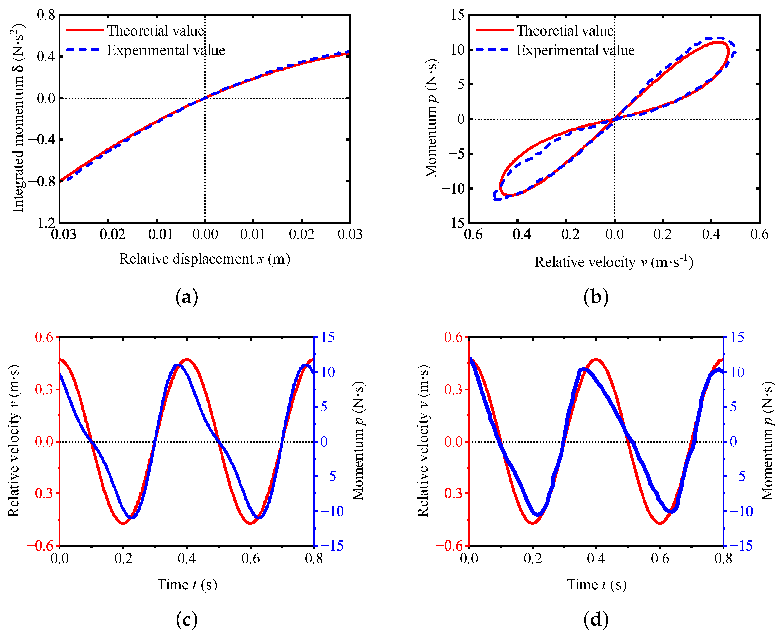
The structural parameters of the fluid mem-inerter device are demonstrated in

Table 1. Structural parameters of the mem-inerter prototype.

Parameter	Value
Piston diameter D	$0.05\mathrm{m}$
Piston rod diameter d	$0.02\mathrm{m}$
Helical channel radius $r_{\mathrm{h}}$	$0.006\mathrm{m}$
Helix pitch $P_{\mathrm{h}}$	$0.014\mathrm{m}$
Piston width w	$0.1\mathrm{m}$
Fluid density $\rho$	$760\mathrm{kg}·{\mathrm{m}}^{-3}$

, and the memory characteristic curves obtained by numerical simulation are compared with the experimental data, as shown in Figure 6.

Figure 6a shows a one-to-one correspondent relationship in the integrated momentum versus displacement plane, which is also the constitutive relationship plane of the mem-inerter, and the curve shows significant nonlinearity. Plotting the loci of $\left(p\right(t),v(t\left)\right)$ in the $p-v$ plane, as shown in Figure 6b, one can obtain the pinched hysteresis loop, which has been identified as the fingerprint of memory elements. Observe from Figure 6c,d that whenever the waveform of the velocity $v\left(t\right)$ crosses the time axis, the waveform of the momentum $p\left(t\right)$ must cross the time axis at the same instants of time. Such a feature is called the coincident zero-crossing signature by Chua, which is a more general experimental memory element identification scheme. Comparing the theoretical data and experimental data in Figure 6, although the curves are not smooth, the memory characteristics can still be identified and it is also in good agreement with the theoretical data.

6.2. Mathematical Modeling

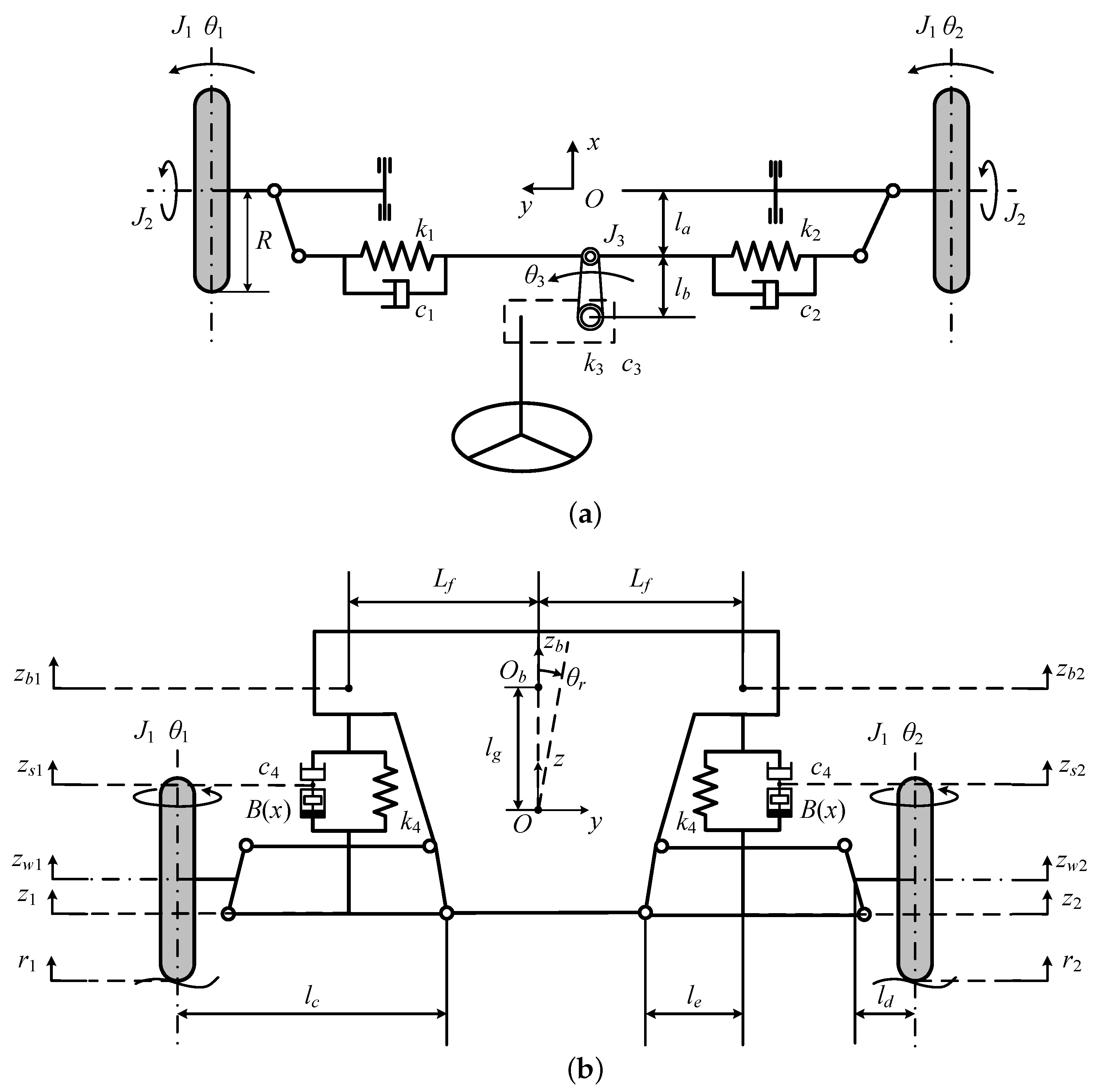
The mechanical model of the vehicle shimmy system equipped with mem-inerters and the parameters related to the structural dimensions of the vehicle marked on the model are shown in Figure 7. In which, O represents the center of gravity (COG) of the vehicle shimmy model, while $O_{\mathrm{b}}$ represents the COG of the sprung mass:

$L_f$ is half of the distance between the two connection points of the front suspension and the vehicle body; $l_a$ is the moment arm of the steering rod acting on the kingpin; $l_b$ is the moment arm of the steering tie rod acting on the pitman arm; $l_c$ is the length of the lateral swing arm of front suspension; $l_d$ is the distance from the intersection point of the kingpin extension line and the ground to the wheel symmetry plane; $l_e$ is the horizontal distance between the connection point between the suspension and the vehicle body and the connection point between the vehicle body and the suspension arm; $l_g$ is the vertical distance between the O and $O_{\mathrm{b}}$; R is the diameter of the wheels.

The shimmy model has seven degrees of freedom (DOF): ${\theta }_1$ and ${\theta }_2$ are the shimmy angles of the left and right front wheel, ${\theta }_3$ is the swing angle of the pitman arm, $z_{\mathrm{b}}$ is the vertical displacement of the sprung mass, $z_{\mathrm{w}1}$ and $z_{\mathrm{w}2}$ are the vertical displacements of the left and right front wheel, and ${\theta }_r$ is the roll angle of the vehicle body. In addition, $z_{\mathrm{s}1}$ and $z_{\mathrm{s}2}$ denote the vertical displacement of the nodes between the mem-inerter and the damper of left and right front suspension

The mathematical model of vehicle shimmy with mem-inerters can be formulated via the integrated Lagrangian equations, which can expressed as

$$\frac{\mathrm{d}}{\mathrm{d}t}(\frac{\mathrm{d}}{\mathrm{d}t}\frac{\partial \overline{\mathcal{L}}}{\partial {\dot{q}}_i}-\frac{\partial \overline{\mathcal{L}}}{\partial q_i}+\frac{\partial \overline{\mathcal{D}}}{\partial {\dot{q}}_i})=Q_i,i=1,2,3,\dots ,9.$$

(58)

where $\overline{\mathcal{L}}={\overline{T}}^{*}-\overline{V}$, ${\overline{T}}^{*}$ represents the integrated kinetic co-energy of the system, $\overline{V}$ represents the integrated potential energy of the system, $\overline{\mathcal{D}}$ represents the integrated dissipative energy of the system, $Q_i$ represents the generalized force acting on each DOF of the system, and $q_i$ represents the generalized coordinate of the system, which is as follows: $[q_1{q}_2\cdots q_9]=\left[{\theta }_1{\theta }_2{\theta }_3{z}_{\mathrm{b}}{z}_{\mathrm{w}1}{z}_{\mathrm{w}2}{z}_{\mathrm{s}1}{z}_{\mathrm{s}2}{\theta }_r\right]$.

Let ${\rho }_i$, ${\zeta }_i$, $u_i$, and ${\xi }_i$ denote the time integrals of angle ${\theta }_i$, vertical displacement $z_i$, running speed $v_i$, and road displacement excitation $r_i$ of the system, respectively,

$${\rho }_i={\int }_0^t{\theta }_i\mathrm{d}\tau ,i=1,2,3,r,$$

(59)

$${\zeta }_i={\int }_0^t{z}_i\mathrm{d}\tau ,i=1,2,\mathrm{w}1,\mathrm{w}2,\mathrm{s}1,\mathrm{s}2,\mathrm{b}1,\mathrm{b}2,\mathrm{b},$$

(60)

$$u_i={\int }_0^t{v}_i\mathrm{d}\tau ,i=1,2,$$

(61)

$${\xi }_i={\int }_0^t{r}_i\mathrm{d}\tau ,i=1,2,$$

(62)

The integrated kinetic energy of the system can be expressed as

$$\begin{array}{cc}\hfill \overline{T}=& \frac{1}{2}{J}_1{\dot{\rho }}_1^2+\frac{1}{2}{J}_2{\left(\frac{u_1}{R}\right)}^2+\frac{1}{2}{m}_{\mathrm{w}}{u}_1^2+\frac{1}{2}{m}_{\mathrm{w}}{\dot{\zeta }}_{\mathrm{w}}^2+\frac{1}{2}{J}_1{\dot{\rho }}_2^2+\frac{1}{2}{J}_2{\left(\frac{u_2}{R}\right)}^2\hfill \\ \hfill & +\frac{1}{2}{m}_{\mathrm{w}}{u}_2^2+\frac{1}{2}{m}_{\mathrm{w}}{\dot{\zeta }}_{\mathrm{w}}^2+\frac{1}{2}{J}_3{\dot{\rho }}_3^2+{\int }_0^{{\dot{\zeta }}_1-{\dot{\zeta }}_{s1}}\delta \left(x\right)\mathrm{d}x+{\int }_0^{{\dot{\zeta }}_2-{\dot{\zeta }}_{s2}}\delta \left(x\right)\mathrm{d}x\hfill \\ \hfill & +\frac{1}{2}{m}_{\mathrm{b}}{u}^2+\frac{1}{2}{m}_{\mathrm{b}}{\dot{\zeta }}_{\mathrm{b}}^2+\frac{1}{2}{m}_{\mathrm{b}}{\left(l_{\mathrm{g}}{\dot{\rho }}_r\right)}^2+\frac{1}{2}{J}_{br}{\dot{\rho }}_r^2,\hfill \end{array}$$

(63)

where $J_1$ and $J_2$ are the inertia moments of front wheels around diameters and spin axes, respectively; $J_3$ is the inertia moment of the pitman arm; $J_{br}$ is the inertia moment of the sprung mass about its roll axis; $m_{\mathrm{b}}$ and $m_{\mathrm{w}}$ are the mass of sprung mass and wheels, respectively.

The integrated potential energy of the system can be given by

$$\begin{array}{cc}\hfill \overline{V}=& \frac{1}{2}{k}_1{(l_a{\rho }_1-l_b{\rho }_3)}^2+\frac{1}{2}{k}_2{(l_a{\rho }_2-l_b{\rho }_3)}^2+\frac{1}{2}{k}_3{\rho }_3^2+\frac{1}{2}{k}_{\mathrm{t}}{({\xi }_1-{\zeta }_{\mathrm{w}1})}^2\hfill \\ \hfill & +\frac{1}{2}{k}_{\mathrm{t}}{({\xi }_2-{\zeta }_{\mathrm{w}2})}^2+\frac{1}{2}{k}_4{(\frac{l_e}{l_c-l_d}{\zeta }_{\mathrm{w}1}-{\zeta }_b-L_f{\rho }_r)}^2\hfill \\ \hfill & +\frac{1}{2}{k}_4{(\frac{l_e}{l_c-l_d}{\zeta }_{\mathrm{w}2}-{\zeta }_{\mathrm{b}}+L_f{\rho }_r)}^2-\frac{1}{2}{m}_g{l}_g{{\rho }_r}^2,\hfill \end{array}$$

(64)

where $k_1$ and $k_2$ denote the stiffness of left and right steering tie rods, respectively; $k_3$ denotes the stiffness of the pitman arm; $k_4$ denotes the stiffness of the front suspensions; $k_{\mathrm{t}}$ denotes the tire vertical stiffness.

The integrated dissipative energy can be expressed as

$$\begin{array}{cc}\hfill \overline{\mathcal{D}}=& \frac{1}{2}{c}_e({{\dot{\rho }}_1}^2+{{\dot{\rho }}_2}^2)+\frac{1}{2}{c}_1{(l_a{\dot{\rho }}_1-l_b{\dot{\rho }}_3)}^2+\frac{1}{2}{c}_2{(l_a{\dot{\rho }}_2-l_b{\dot{\rho }}_3)}^2+\frac{1}{2}{c}_3{\dot{\rho }}_3^2\hfill \\ \hfill & +\frac{1}{2}{c}_4{({\dot{\zeta }}_{\mathrm{s}1}-{\dot{\zeta }}_{\mathrm{b}}-L_f{\dot{\rho }}_r)}^2+\frac{1}{2}{c}_4{({\dot{\zeta }}_{\mathrm{s}2}-{\dot{\zeta }}_{\mathrm{b}}+L_f{\dot{\rho }}_r)}^2,\hfill \end{array}$$

(65)

where $c_e$ is the equivalent damping of front wheels around their kingpins; $c_1$ and $c_2$ are the damping of left and right steering tie rods, respectively; $c_3$ is the damping of the pitman arm; $c_4$ is the damping of front suspension.

The generalized forces corresponding to each DOF of the system can be expressed as

$$\begin{array}{cc}\hfill & Q_{{\theta }_1}=-F_{Y1}(R\gamma +e),\hfill \\ \hfill & Q_{{\theta }_2}=-F_{Y2}(R\gamma +e),\hfill \\ \hfill & Q_{{\theta }_3}=0,\hfill \\ \hfill & Q_{zw1}=-k_{\mathrm{t}}{l}_d\gamma {\theta }_1,\hfill \\ \hfill & Q_{zw2}=k_{\mathrm{t}}{l}_d\gamma {\theta }_2,\hfill \\ \hfill & Q_{zb}=0,\hfill \\ \hfill & Q_{\theta r}=0,\hfill \end{array}$$

(66)

where $F_{Y1}$ and $F_{Y2}$ represent the lateral forces of the front wheels, respectively, and e represent the pneumatic trail of the tire.

Substituting (59)–(66) into (58), the differential equations of the system can be derived as follows:

$$J_1{\ddot{\theta }}_1+(c_e+c_1{l_a}^2){\dot{\theta }}_1+k_1{l}_a^2{\theta }_1-c_1{l}_a{l}_b{\dot{\theta }}_3-k_1{l}_a{l}_b{\theta }_3+F_{Y1}(R\gamma +e)=0,$$

(67)

$$J_1{\ddot{\theta }}_2+(c_e+c_2{l_a}^2){\dot{\theta }}_2+k_2{l}_a^2{\theta }_2-c_2{l}_a{l}_b{\dot{\theta }}_3-k_2{l}_a{l}_b{\theta }_3+F_{Y2}(R\gamma +e)=0,$$

(68)

$$J_3{\ddot{\theta }}_3+(c_1{l}_b^2+c_2{l}_b^2+c_3){\dot{\theta }}_3+(k_1{l}_b^2+k_2{l}_b^2+k_3){\theta }_3-c_1{l}_a{l}_b{\dot{\theta }}_1-c_2{l}_a{l}_b{\dot{\theta }}_2-k_1{l}_a{l}_b{\theta }_1-k_2{l}_a{l}_b{\theta }_2=0,$$

(69)

$$\begin{array}{c}\hfill m_{\mathrm{w}}{\ddot{z}}_{\mathrm{w}1}+\frac{l_e}{l_c-l_d}B(\frac{l_e}{l_c-l_d}{z}_{\mathrm{w}1}-z_{\mathrm{s}1})(\frac{l_e}{l_c-l_d}{\ddot{z}}_{\mathrm{w}1}-{\ddot{z}}_{\mathrm{s}1})+\frac{l_e}{l_c-l_d}\dot{B}(\frac{l_e}{l_c-l_d}{z}_{\mathrm{w}1}-z_{\mathrm{s}1})(\frac{l_e}{l_c-l_d}{\dot{z}}_{\mathrm{w}1}-{\dot{z}}_{\mathrm{s}1})\\ \hfill +k_{\mathrm{t}}(z_{\mathrm{w}1}-q_1)+k_4\frac{l_e}{l_c-l_d}(\frac{l_e}{l_c-l_d}{z}_{\mathrm{w}1}-z_{\mathrm{b}}-L_f{\theta }_r)-k_{\mathrm{t}}{l}_d\gamma {\theta }_1=0,\end{array}$$

(70)

$$\begin{array}{c}\hfill m_{\mathrm{w}}{\ddot{z}}_{{\mathrm{w}}_2}+\frac{l_e}{l_c-l_d}B(\frac{l_e}{l_c-l_d}{z}_{\mathrm{w}2}-z_{\mathrm{s}2})(\frac{l_e}{l_c-l_d}{\ddot{z}}_{{\mathrm{w}}_2}-{\ddot{z}}_{\mathrm{s}2})+\frac{l_e}{l_c-l_d}\dot{B}(\frac{l_e}{l_c-l_d}{z}_{\mathrm{w}2}-z_{\mathrm{s}2})(\frac{l_e}{l_c-l_d}{\dot{z}}_{\mathrm{w}2}-{\dot{z}}_{\mathrm{s}2})\\ \hfill +k_{\mathrm{t}}(z_{\mathrm{w}2}-q_2)+k_4\frac{l_e}{l_c-l_d}(\frac{l_e}{l_c-l_d}{z}_{\mathrm{w}2}-z_{\mathrm{b}}+L_f{\theta }_r)+k_{\mathrm{t}}{l}_d\gamma {\theta }_2=0,\end{array}$$

(71)

$$m_{\mathrm{b}}{\ddot{z}}_{\mathrm{b}}-c_4({\dot{z}}_{\mathrm{s}1}-{\dot{z}}_{\mathrm{b}})-c_4({\dot{z}}_{\mathrm{s}2}-{\dot{z}}_{\mathrm{b}})-k_4(\frac{l_e}{l_c-l_d}{z}_{\mathrm{w}1}-z_{\mathrm{b}})-k_4(\frac{l_e}{l_c-l_d}{z}_{\mathrm{w}2}-z_{\mathrm{b}})=0,$$

(72)

$$(m_{\mathrm{b}}{l_g}^2+J_{br}){\ddot{\theta }}_r-c_4{L}_f({\dot{z}}_{\mathrm{s}1}-L_f{\dot{\theta }}_r)+c_4{L}_f({\dot{z}}_{\mathrm{s}2}+L_f{\dot{\theta }}_r)-k_4{L}_f(\frac{l_e}{l_c-l_d}{z}_{\mathrm{w}1}-L_f{\theta }_r)+k_4{L}_f(\frac{l_e}{l_c-l_d}{z}_{\mathrm{w}2}+L_f{\theta }_r)-m_{\mathrm{b}}{l}_g{\theta }_r=0,$$

(73)

In the study of vehicle shimmy, tires are also an important factor. Therefore, Pacejka’s Magic Formula [36] is chosen as the nonlinear tire model in this study, and the tire lateral force can be represented in the form

$$F_Y=Dsin\{Carctan[B(1-E)(\alpha +S_H)+EarctanB(\alpha +S_H)]\}+S_V,$$

(74)

where $\alpha$ is the slip angle of the wheel, B is the stiffness factor, C is the shape factor, D is the peak value, E is the curvature factor, $S_H$ is the horizontal shift, and $S_V$ is the vertical shift. Here, let $S_H=0$ and $S_V=0$, and parameters B, C, D and E can be calculated by

$$\begin{array}{cc}\hfill & C=p_{C1},\hfill \\ \hfill & D=p_{D1}{F}_z^2+p_{D2},\hfill \\ \hfill & BCD=p_{BCD1}sin(2arctan\frac{F_z}{p_{BCD2}})(1-p_{BCD3}\left|\phi \right|),\hfill \\ \hfill & B=\frac{BCD}{C·D},\hfill \\ \hfill & E=p_{E1}{F}_z+p_{E2},\hfill \end{array}$$

(75)

where $F_z$ is the vertical load acting on the wheels, $\phi$ is the camber angle of the wheels, and the parameters $p_{C1}$, $p_{D1}$, $p_{D2}$, $p_{BCD1}$, $p_{BCD2}$, $p_{BCD3}$, $p_{E1}$, and $p_{E2}$ are all constants determined for each tire. In this study, the value of $\phi$ is 0, and the values of $p_{C1}$, $p_{D1}$, $p_{D2}$, $p_{BCD1}$, $p_{BCD2}$, $p_{BCD3}$, $p_{E1}$, and $p_{E2}$ are listed in

Table 2. Coefficient values of Magic Formula.

Parameter	Value
$p_{C1}$	1.6500
$P_{D1}$	−34.00
$p_{D2}$	1250.00
$p_{E1}$	−0.0210
$p_{E2}$	0.7739
$p_{BCD1}$	3036.00
$p_{BCD2}$	12.80
$p_{BCD3}$	0.0050

[37,38,39].

Assuming that the vehicle has no lateral acceleration, the vertical loads acting on the left-front wheel $F_{z1}$ and the right-front wheel $F_{z2}$ are as follows:

$$\begin{array}{c}\hfill F_{z1}=F_{f0}-k_{\mathrm{t}}(z_{\mathrm{w}1}-q_1),\\ \hfill F_{z2}=F_{f0}-k_{\mathrm{t}}(z_{\mathrm{w}2}-q_2),\end{array}$$

(76)

where $F_{f0}$ is the static vertical load acting on the front wheels, which can be obtained by

$$F_{f0}=\frac{1}{2}\frac{a}{a+b}(m_{\mathrm{b}}+4m_{\mathrm{w}})g,$$

(77)

where a and b represent the distance from the COG of the vehicle to its front and rear axle, respectively.

The constrain between the slip angle and the shimmy angle of the front wheel can be given as

$$\begin{array}{c}\hfill {\dot{\alpha }}_1+\frac{v}{\sigma }{\alpha }_1+\frac{v}{\sigma }{\theta }_1-\frac{a_m}{\sigma }{\dot{\theta }}_1=0,\\ \hfill {\dot{\alpha }}_2+\frac{v}{\sigma }{\alpha }_2+\frac{v}{\sigma }{\theta }_2-\frac{a_m}{\sigma }{\dot{\theta }}_2=0,\end{array}$$

(78)

where $\sigma$ is the relaxation length of tires and $a_m$ is the half-length of the tire contact area. In this study, $\sigma$ is equal to $0.65\mathrm{m}$ and $a_m$ is equal to $0.2\mathrm{m}$.

6.3. Simulation Analysis

To verify the accuracy improvement of the integrated Lagrangian method in modeling the vehicle shimmy system with mem-inerters and to study the influence factor of error between the Lagrangian method and integrated Lagrangian method, simulation analysis and comparison are performed under pulse and random excitation, respectively.

Body acceleration, suspension working space, dynamic tire load, body roll angle acceleration, the shimmy angle of the front wheels and the swing angle of the pitman arm, which are the main evaluation indicators of a vehicle shimmy model, are selected as comparison indicators in simulation analysis. For the sake of conciseness, the body acceleration, suspension working space, dynamic tire load, and body roll angle acceleration are abbreviated as BA, SWS, DTL, and BRAA, respectively.

Let $m_{2\mathrm{F}}=960\mathrm{kg}$, $m_{2\mathrm{H}}=780\mathrm{kg}$ and $m_{2\mathrm{N}}=600\mathrm{kg}$ represent the sprung mass under full-load, half-load and no-load conditions, respectively. In addition, the value of the remaining vehicle parameters are listed in

Table 3. Parameter values of the vehicle shimmy system.

Parameter	Value
Inertia moment of front wheels around diameters $J_1$	$8\mathrm{kg}·{\mathrm{m}}^2$
Inertia moment of front wheels around spin axes $J_2$	$6\mathrm{kg}·{\mathrm{m}}^2$
Inertia moment of pitman arm $J_3$	$3\mathrm{kg}·{\mathrm{m}}^2$
Mass of wheels $m_{\mathrm{w}}$	$45\mathrm{kg}$
Distance from the COG of the vehicle to its front axle a	$1.22\mathrm{m}$
Distance from the COG of the vehicle to its rear axle b	$1.473\mathrm{m}$
Half of the distance between the two connection points of the front suspension and the vehicle body $L_f$	$0.37\mathrm{m}$
Stiffness of left steering tie rod $k_1$	$2240\mathrm{kN}·{\mathrm{m}}^{-1}$
Stiffness of right steering tie rod $k_2$	$2240\mathrm{kN}·{\mathrm{m}}^{-1}$
Stiffness of pitman arm $k_3$	$60\mathrm{kN}·{\mathrm{m}}^{-1}$
Stiffness of front suspensions $k_4$	$22\mathrm{kN}·{\mathrm{m}}^{-1}$
Tire vertical stiffness $k_{\mathrm{t}}$	$192\mathrm{kN}·{\mathrm{m}}^{-1}$
Damping of left steering tie rod $c_1$	$630\mathrm{N}·\mathrm{m}·{\mathrm{s}}^{-1}$
Damping of right steering tie rod $c_2$	$630\mathrm{N}·\mathrm{m}·{\mathrm{s}}^{-1}$
Damping of pitman arm $c_3$	$100\mathrm{N}·\mathrm{m}·{\mathrm{s}}^{-1}$
Damping of front suspension $c_4$	$4500\mathrm{N}·\mathrm{m}·{\mathrm{s}}^{-1}$
Equivalent damping of front wheels around their kingpins $c_e$	$44\mathrm{N}·\mathrm{m}·{\mathrm{s}}^{-1}$
Caster angle of front wheels $\gamma$	$0.06\mathrm{rad}$
Diameter of the wheels R	$0.4\mathrm{m}$
Moment arm of force of steering rod acting on kingpin $l_a$	$0.125\mathrm{m}$
Moment arm of force of steering tie rod acting on pitman arm $l_b$	$0.1\mathrm{m}$
Lateral swing arm of front suspension $l_c$	$0.612\mathrm{m}$
Distance from the intersection point of the kingpin extension line and the ground to the symmetry plane of the wheel $l_d$	$0.2\mathrm{m}$
Horizontal distance between the suspension and the connection points of the vehicle body and suspension arm $l_e$	$0.14\mathrm{m}$
Vertical displacement between O and $O_{\mathrm{b}}$ $l_g$	$0.55\mathrm{m}$
Pneumatic trail of tire e	$0.07\mathrm{m}$

.

First, consider a pulse excitation of the form

$$q\left(t\right)=\frac{A}{2}(1-cos\frac{v}{l}2\pi t)0⩽t⩽\frac{l}{v},$$

(79)

where $v=10\mathrm{m}·{\mathrm{s}}^{-1}$, $A=0.08\mathrm{m}$, and $t=5\mathrm{s}$.

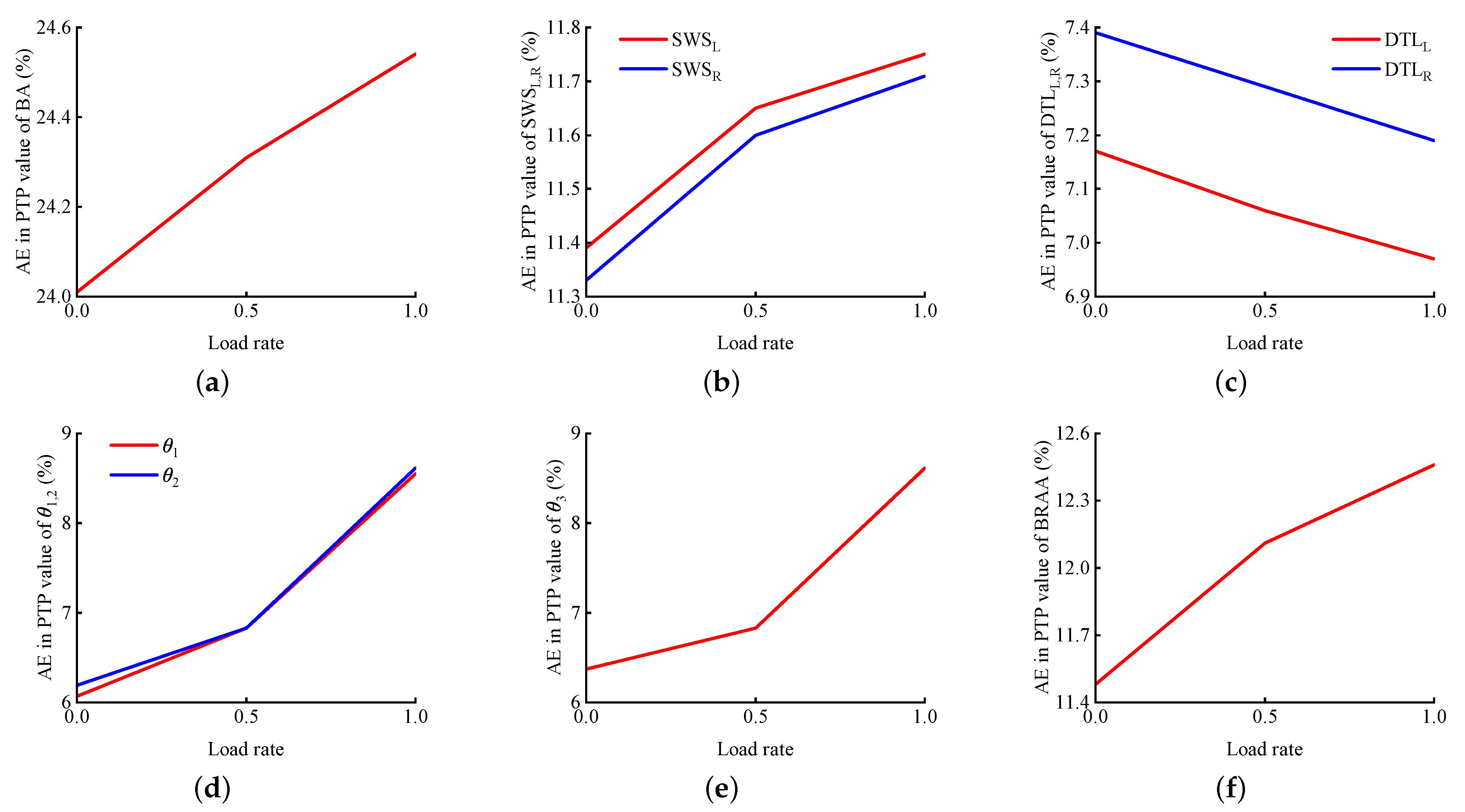
The time-domain responses of the system under no-load, half-load, and full-load conditions are studied, respectively. To avoid redundancy, only the results for the no-load case are shown in Figure 8. The peak-to-peak (PTP) values, calculated from $\max x\left(t\right)-\min x\left(t\right)$, where $x\left(t\right)$ denote the values of the signal in a period and the absolute value of the error (abbreviated as AE), are listed in

Table 4. The absolute values of PTP value error of time-domain responses between the Lagrangian and the integrated Lagrangian methods under pulse excitation.

Vehicle Load	Indicator	Integrated Lagrangian Method	Lagrangian Method	Absolute Value of Error
No-load	$\mathrm{BA}/\mathrm{m}·{\mathrm{s}}^{-2}$	9.4783	11.7546	24.01%
	${\mathrm{SWS}}_{\mathrm{L}}/\mathrm{m}$	0.078	0.0691	11.39%
	${\mathrm{SWS}}_{\mathrm{R}}/\mathrm{m}$	0.0781	0.0692	11.33%
	${\mathrm{DTL}}_{\mathrm{L}}/\mathrm{kN}$	3.5971	3.3392	7.17%
	${\mathrm{DTL}}_{\mathrm{R}}/\mathrm{kN}$	3.3586	3.1106	7.39%
	${\theta }_1/\mathrm{rad}$	0.0509	0.0478	6.07%
	${\theta }_2/\mathrm{rad}$	0.0497	0.0466	6.19%
	${\theta }_3/\mathrm{rad}$	0.0277	0.0259	6.37%
	$\mathrm{BRAA}/\mathrm{rad}·{\mathrm{s}}^{-2}$	0.1608	0.1424	11.48%
Half-load	$\mathrm{BA}/\mathrm{m}·{\mathrm{s}}^{-2}$	8.1265	10.1024	24.31%
	${\mathrm{SWS}}_{\mathrm{L}}/\mathrm{m}$	0.089	0.0787	11.65%
	${\mathrm{SWS}}_{\mathrm{R}}/\mathrm{m}$	0.0893	0.0789	11.60%
	${\mathrm{DTL}}_{\mathrm{L}}/\mathrm{kN}$	3.8765	3.6027	7.06%
	${\mathrm{DTL}}_{\mathrm{R}}/\mathrm{kN}$	3.6253	3.3611	7.29%
	${\theta }_1/\mathrm{rad}$	0.0548	0.0511	6.83%
	${\theta }_2/\mathrm{rad}$	0.0537	0.05	6.86%
	${\theta }_3/\mathrm{rad}$	0.0299	0.0278	6.83%
	$\mathrm{BRAA}/\mathrm{rad}·{\mathrm{s}}^{-2}$	0.1884	0.1656	12.11%
Full-load	$\mathrm{BA}/\mathrm{m}·{\mathrm{s}}^{-2}$	7.0558	8.7876	24.54%
	${\mathrm{SWS}}_{\mathrm{L}}/\mathrm{m}$	0.0965	0.0851	11.75%
	${\mathrm{SWS}}_{\mathrm{R}}/\mathrm{m}$	0.0968	0.0855	11.71%
	${\mathrm{DTL}}_{\mathrm{L}}/\mathrm{kN}$	4.0503	3.768	6.97%
	${\mathrm{DTL}}_{\mathrm{R}}/\mathrm{kN}$	3.7962	3.523	7.19%
	${\theta }_1/\mathrm{rad}$	0.0623	0.057	8.55%
	${\theta }_2/\mathrm{rad}$	0.0611	0.0559	8.57%
	${\theta }_3/\mathrm{rad}$	0.0341	0.0312	8.61%
	$\mathrm{BRAA}/\mathrm{rad}·{\mathrm{s}}^{-2}$	0.2184	0.1912	12.46%

and are shown as a line chart in Figure 9.

Based on the data shown in Figure 8 and Table 4, compared with the integrated Lagrangian method (i.e., accurate values), each system indicator modeled using the Lagrangian method for the vehicle shimmy system with mem-inerters exhibits errors ranging from $6.07\%$ to $24.54\%$. Such errors indicate that modeling mechanical systems equipped with memory elements using the Lagrangian method is inaccurate and cannot accurately represent the dynamical behavior of the systems. Furthermore, it can be seen from Table 4 and Figure 9 that, under pulse excitation, as the vehicle load increases, the PTP value errors in body acceleration, suspension working space, shimmy angle of the front wheels, swing angle of the pitman arm, and body roll angle acceleration increase, and the PTP value error of dynamic tire load decreases.

Since the road excitation is usually random, a time-domain model of random road excitation is established to discuss the errors of the system response obtained by these two modeling methods under random road excitation

$$\dot{q}\left(t\right)=-2\pi f_{0}q\left(t\right)+2\pi \sqrt{G_{0}v}w\left(t\right),$$

(80)

where $f_0$ is the cut-off frequency, $G_0$ is the road unevenness coefficient, and v is the vehicle speed, $\omega \left(t\right)$ is the integrated white noise. In this study, four cases are investigated, namely, (1) Class A road profile, vehicle speed $v=30\mathrm{m}·{\mathrm{s}}^{-1}$, no-load; (2) Class B road profile, vehicle speed $v=20\mathrm{m}·{\mathrm{s}}^{-1}$, no-load; (3) Class B road profile, vehicle speed $v=30\mathrm{m}·{\mathrm{s}}^{-1}$, no-load; (4) Class B road profile, vehicle speed $v=30\mathrm{m}·{\mathrm{s}}^{-1}$, full-load.

To avoid redundancy, only the results for case (2) are presented in Figure 10. The RMS values and the absolute value of errors of the time-domain response using the Lagrangian method and the integrated Lagrangian method are shown in

Table 5. The absolute values of RMS value error of time-domain response between the Lagrangian and the integrated Lagrangian methods under random excitation.

Case	Condition	Indicator	Integrated Lagrangian Method	Lagrangian Method	Absolute Value of Error
1	Class A road	$\mathrm{BA}/\mathrm{m}·{\mathrm{s}}^{-2}$	0.4655	0.5137	10.35%
	$v=30\mathrm{m}·{\mathrm{s}}^{-1}$	${\mathrm{SWS}}_{\mathrm{L}}/\mathrm{m}$	0.0039	0.0035	8.85%
	No-load	${\mathrm{SWS}}_{\mathrm{R}}/\mathrm{m}$	0.0027	0.0024	9.89%
		${\mathrm{DTL}}_{\mathrm{L}}/\mathrm{kN}$	0.2577	0.2444	5.16%
		${\mathrm{DTL}}_{\mathrm{R}}/\mathrm{kN}$	0.2005	0.1901	5.17%
		${\theta }_1/\mathrm{rad}$	0.0054	0.0047	13.53%
		${\theta }_2/\mathrm{rad}$	0.0052	0.0045	12.22%
		${\theta }_3/\mathrm{rad}$	0.0029	0.0025	13.06%
		$\mathrm{BRAA}/\mathrm{rad}·{\mathrm{s}}^{-2}$	0.2258	0.1964	13.02%
2	Class B road	$\mathrm{BA}/\mathrm{m}·{\mathrm{s}}^{-2}$	0.7616	0.8431	10.71%
	$v=20\mathrm{m}·{\mathrm{s}}^{-1}$	${\mathrm{SWS}}_{\mathrm{L}}/\mathrm{m}$	0.0066	0.0059	10.95%
	No-load	${\mathrm{SWS}}_{\mathrm{R}}/\mathrm{m}$	0.0046	0.004	13.13%
		${\mathrm{DTL}}_{\mathrm{L}}/\mathrm{kN}$	0.418	0.396	5.27%
		${\mathrm{DTL}}_{\mathrm{R}}/\mathrm{kN}$	0.3234	0.3059	5.44%
		${\theta }_1/\mathrm{rad}$	0.0087	0.0075	13.72%
		${\theta }_2/\mathrm{rad}$	0.0083	0.0071	13.63%
		${\theta }_3/\mathrm{rad}$	0.0046	0.004	13.39%
		$\mathrm{BRAA}/\mathrm{rad}·{\mathrm{s}}^{-2}$	0.3727	0.3234	13.23%
3	Class B road	$\mathrm{BA}/\mathrm{m}·{\mathrm{s}}^{-2}$	0.9309	1.0315	10.81%
	$v=30\mathrm{m}·{\mathrm{s}}^{-1}$	${\mathrm{SWS}}_{\mathrm{L}}/\mathrm{m}$	0.0078	0.0068	12.18%
	No-load	${\mathrm{SWS}}_{\mathrm{R}}/\mathrm{m}$	0.0054	0.0046	14.94%
		${\mathrm{DTL}}_{\mathrm{L}}/\mathrm{kN}$	0.5092	0.4821	5.32%
		${\mathrm{DTL}}_{\mathrm{R}}/\mathrm{kN}$	0.3938	0.3719	5.55%
		${\theta }_1/\mathrm{rad}$	0.0106	0.0091	13.89%
		${\theta }_2/\mathrm{rad}$	0.0101	0.0087	14.05%
		${\theta }_3/\mathrm{rad}$	0.0056	0.0048	13.59%
		$\mathrm{BRAA}/\mathrm{rad}·{\mathrm{s}}^{-2}$	0.4513	0.3901	13.57%
4	Class B road	$\mathrm{BA}/\mathrm{m}·{\mathrm{s}}^{-2}$	0.5912	0.6566	11.06%
	$v=30\mathrm{m}·{\mathrm{s}}^{-1}$	${\mathrm{SWS}}_{\mathrm{L}}/\mathrm{m}$	0.0096	0.0082	15.18%
	Full-load	${\mathrm{SWS}}_{\mathrm{R}}/\mathrm{m}$	0.0065	0.0054	17.23%
		${\mathrm{DTL}}_{\mathrm{L}}/\mathrm{kN}$	0.503	0.475	5.56%
		${\mathrm{DTL}}_{\mathrm{R}}/\mathrm{kN}$	0.3877	0.3646	5.95%
		${\theta }_1/\mathrm{rad}$	0.0131	0.012	8.16%
		${\theta }_2/\mathrm{rad}$	0.0129	0.0111	13.55%
		${\theta }_3/\mathrm{rad}$	0.0073	0.0068	7.02%
		$\mathrm{BRAA}/\mathrm{rad}·{\mathrm{s}}^{-2}$	0.4516	0.3897	13.71%

. According to Figure 10 and Table 5, compared with the integrated Lagrangian method, each of the system indicators modeled using the Lagrangian method for the vehicle shimmy system with mem-inerters results in errors ranging from $5.17\%$ to $17.23\%$. This reaffirms the previous finding that modeling mechanical systems equipped with memory elements using the Lagrangian method is inaccurate and cannot accurately represent the dynamical behavior of such systems.

To study the influence of road roughness, vehicle speed, and load condition on the RMS value errors of system time-domain response under random excitation, the results are plotted in Figure 11, Figure 12 and Figure 13. As can be seen from Figure 11 and the data of cases (1) and (3) in Table 5, the RMS value errors for each indicator between the Lagrangian method and the integrated Lagrangian method increase as the road unevenness increases, i.e., as the road condition deteriorates.

As shown in Figure 12 and the data of cases (2) and (3) in Table 5, the RMS value errors for each indicator between the Lagrangian method and the integrated Lagrangian method increase as the vehicle speed increases.

Figure 13 and the data of case (3) and (4) in Table 5 show that, under random excitation, the RMS value error of BA, SWS, DTL, BRAA increase, the RMS value error of ${\theta }_1$ and ${\theta }_3$ decrease, and the RMS value error of ${\theta }_2$ increases and then decreases with the increase in the vehicle load, where load rates of 0, 0.5, and 1 indicate no load, a half load, and a full load, respectively. The abnormal changes in ${\theta }_2$ may be due to the complex nonlinearity of the system, which needs to be analyzed in future research.

7. Conclusions

In this paper, a novel modeling method, referred to as the integrated Lagrangian modeling method, is proposed to accurately describe the nonlinear dynamic behavior of the mechanical systems consisting of mem-inerters, mem-springs, and mem-dampers, together with their conventional linear counterparts. Based on the constitutive relationships of memory elements, the corresponding memory state functions are introduced, and then the Lagrangian of the system can be obtained based on the difference between two memory-state functions. In the case of a mechanical system that consists only of mem-inerters, mem-springs, and their conventional linear counterparts, the dynamic equations can be obtained from Hamilton’s least action principle. Mem-dampers and linear damping elements can be included by introducing an action function that plays a role similar to the Rayleigh dissipation function. Furthermore, this paper also briefly generalizes memory elements and their modeling to fractional calculus.

By comparing the results of using the classical Lagrangian method and the integrated Lagrangian method to model the vehicle shimmy system equipped with the fluid mem-inerter, the modeling accuracy improvement of the integrated Lagrangian method is verified. The results show that

• Under pulse and random road excitation, there are obvious errors in each indicator of system modeling using the Lagrangian method compared to the results obtained using the integrated Lagrangian method (accurate values). The existence of such errors demonstrates the accuracy and necessity of using the integrated Lagrangian method to model mechanical systems with memory elements.
• Under pulse excitation, as the vehicle load increases, the PTP value errors of BA, ${\mathrm{SWS}}_{\mathrm{L},\mathrm{R}}$, ${\theta }_{1,2}$ and ${\theta }_3$ increase, and the PTP value error of ${\mathrm{DTL}}_{\mathrm{L},\mathrm{R}}$ decreases.
• Under random excitation, the RMS value errors for each indicator increase as the road unevenness increases, i.e., as the road condition deteriorates; the RMS value errors for each indicator increase as the vehicle speed increases; the RMS value errors of BA, ${\mathrm{SWS}}_{\mathrm{L},\mathrm{R}}$, ${\mathrm{DTL}}_{\mathrm{L},\mathrm{R}}$, BRAA increase, the RMS value errors of ${\theta }_1$ and ${\theta }_3$ decrease, and the RMS value error of ${\theta }_2$ increases and then decreases with the increase in the vehicle load.

The integrated Lagrangian method provides a more accurate theoretical method for modeling and analysis of mechanical systems with memory elements. Refs. [6,7] proposed a fluid mem-inerter device and clarified its constitutive relationship in the $\delta -x$ plane. Based on the research of [6,7], this paper applied the mem-inerter to the vehicle suspension system and conducted shimmy modeling analysis, pointing out an easily overlooked problem in that the classical Lagrangian method is not accurate for modeling the mechanical system with memory elements. As a next step, a more in-depth exploration of fractional-order memory elements and the application of fractional-order calculus in modeling mechanical systems with memory elements should be considered, and this method should be integrated with data-driven modeling in future research. Furthermore, the response results of the vehicle shimmy system under pulse and random excitation in the simulation analysis section also need to be experimentally verified in a future study.

References

- Chua, L. Memristor-the missing circuit element. IEEE Trans. Circuit Theory 1971, 18, 507–519. [Google Scholar] [CrossRef]
- Chua, L.O. The fourth element. Proc. IEEE 2012, 100, 1920–1927. [Google Scholar] [CrossRef]
- Itoh, M.; Chua, L.O. Memristor hamiltonian circuits. Int. J. Bifurc. Chaos 2011, 21, 2395–2425. [Google Scholar] [CrossRef]
- Biolek, Z.; Biolek, D.; Biolková, V. Computation of the area of memristor pinched hysteresis loop. IEEE Trans. Circuits Syst. II Express Briefs 2012, 59, 607–611. [Google Scholar] [CrossRef]
- Biolek, Z.; Biolek, D.; Biolková, V.; Kolka, Z. Lagrangian and Hamiltonian formalisms for coupled higher-order elements: Theory, modeling, simulation. Nonlinear Dyn. 2021, 104, 3547–3560. [Google Scholar] [CrossRef]
- Zhang, X.l.; Gao, Q.; Nie, J. The mem-inerter: A new mechanical element with memory. Adv. Mech. Eng. 2018, 10, 1687814018778428. [Google Scholar] [CrossRef]
- Zhang, X.L.; Geng, C.; Nie, J.M.; Gao, Q. The missing mem-inerter and extended mem-dashpot found. Nonlinear Dyn. 2020, 101, 835–856. [Google Scholar] [CrossRef]
- Zhong, Y.; Tang, J.; Li, X.; Gao, B.; Qian, H.; Wu, H. Dynamic memristor-based reservoir computing for high-efficiency temporal signal processing. Nat. Commun. 2021, 12, 408. [Google Scholar] [CrossRef]
- Zhang, X.L.; Zhu, Z.; Nie, J.M.; Liao, Y.G. Mem-inerter: A passive nonlinear element equivalent to the semi-active inerter performing initial-displacement-dependent inertance control strategy. J. Braz. Soc. Mech. Sci. Eng. 2021, 43, 1–14. [Google Scholar] [CrossRef]
- Tour, J.M.; He, T. The fourth element. Nature 2008, 453, 42–43. [Google Scholar] [CrossRef]
- Chua, L.O.; Kang, S.M. Memristive devices and systems. Proc. IEEE 1976, 64, 209–223. [Google Scholar] [CrossRef]
- Chua, L.O. Nonlinear circuit foundations for nanodevices. I. The four-element torus. Proc. IEEE 2003, 91, 1830–1859. [Google Scholar] [CrossRef]
- Strukov, D.B.; Snider, G.S.; Stewart, D.R.; Williams, R.S. The missing memristor found. Nature 2008, 453, 80–83. [Google Scholar] [CrossRef]
- Di Ventra, M.; Pershin, Y.V.; Chua, L.O. Circuit elements with memory: Memristors, memcapacitors, and meminductors. Proc. IEEE 2009, 97, 1717–1724. [Google Scholar] [CrossRef]
- Wang, F.Z. A triangular periodic table of elementary circuit elements. IEEE Trans. Circuits Syst. I Regul. Pap. 2013, 60, 616–623. [Google Scholar] [CrossRef]
- Feali, M.S. Using volatile/non-volatile memristor for emulating the short-and long-term adaptation behavior of the biological neurons. Neurocomputing 2021, 465, 157–166. [Google Scholar] [CrossRef]
- Hu, H.; Scholz, A.; Dolle, C.; Zintler, A.; Quintilla, A.; Liu, Y.; Tang, Y.; Breitung, B.; Marques, G.C.; Eggeler, Y.M.; et al. Inkjet-Printed Tungsten Oxide Memristor Displaying Non-Volatile Memory and Neuromorphic Properties. Adv. Funct. Mater. 2023, 2302290. [Google Scholar] [CrossRef]
- Shen, Z.; Zhao, C.; Qi, Y.; Mitrovic, I.Z.; Yang, L.; Wen, J.; Huang, Y.; Li, P.; Zhao, C. Memristive non-volatile memory based on graphene materials. Micromachines 2020, 11, 341. [Google Scholar] [CrossRef]
- Liu, M.; Cao, Z.; Wang, X.; Mao, S.; Qin, J.; Yang, Y.; Rao, Z.; Zhao, Y.; Sun, B. Perovskite material-based memristors for applications in information processing and artificial intelligence. J. Mater. Chem. C 2023, 11, 13167–13188. [Google Scholar] [CrossRef]
- Matsukatova, A.N.; Iliasov, A.I.; Nikiruy, K.E.; Kukueva, E.V.; Vasiliev, A.L.; Goncharov, B.V.; Sitnikov, A.V.; Zanaveskin, M.L.; Bugaev, A.S.; Demin, V.A.; et al. Convolutional Neural Network Based on Crossbar Arrays of (Co-Fe-B) × (LiNbO3) 100 - x Nanocomposite Memristors. Nanomaterials 2022, 12, 3455. [Google Scholar] [CrossRef]
- Miranda, E.; Suñé, J. Memristors for Neuromorphic Circuits and Artificial Intelligence Applications. Materials 2020, 13, 938. [Google Scholar] [CrossRef] [PubMed]
- Oster, G.F.; Auslander, D.M. The Memristor: A New Bond Graph Element; ASME: New York, NY, USA, 1972. [Google Scholar]
- Nie, J.; Chen, L.; Huang, X.; Wei, H.; Zhang, X. Network synthesis design method of nonlinear suspension system with mem-inerter. J. Vib. Eng. Technol. 2023, 11, 3321–3337. [Google Scholar] [CrossRef]
- Jeltsema, D.; Scherpen, J.M. Multidomain modeling of nonlinear networks and systems. IEEE Control Syst. Mag. 2009, 29, 28–59. [Google Scholar]
- Kelly, S.D.; Hukkeri, R.B. Mechanics, dynamics, and control of a single-input aquatic vehicle with variable coefficient of lift. IEEE Trans. Robot. 2006, 22, 1254–1264. [Google Scholar] [CrossRef]
- Almeshal, A.M.; Goher, K.M.; Tokhi, M.O. Dynamic modelling and stabilization of a new configuration of two-wheeled machines. Robot. Auton. Syst. 2013, 61, 443–472. [Google Scholar] [CrossRef]
- Bao, Y.; Thesma, V.; Kelkar, A.; Velni, J.M. Physics-guided and Energy-based Learning of Interconnected Systems: From Lagrangian to Port-Hamiltonian Systems. In Proceedings of the 2022 IEEE 61st Conference on Decision and Control (CDC), Cancun, Mexico, 6–9 December 2022; pp. 2815–2820. [Google Scholar]
- Bao, Y.; Thesma, V.; Velni, J.M. Physics-guided and neural network learning-based sliding mode control. IFAC-PapersOnLine 2021, 54, 705–710. [Google Scholar] [CrossRef]
- Jeltsema, D. Memory elements: A paradigm shift in Lagrangian modeling of electrical circuits. IFAC Proc. Vol. 2012, 45, 445–450. [Google Scholar] [CrossRef]
- Sun, L.; Chen, Y.; Dang, R.; Cheng, G.; Xie, J. Shifted Legendre polynomials algorithm used for the numerical analysis of viscoelastic plate with a fractional order model. Math. Comput. Simul. 2022, 193, 190–203. [Google Scholar] [CrossRef]
- Di Paola, M.; Reddy, J.; Ruocco, E. On the application of fractional calculus for the formulation of viscoelastic Reddy beam. Meccanica 2020, 55, 1365–1378. [Google Scholar] [CrossRef]
- Wu, J.; Zhang, X.; Liu, L.; Wu, Y. Twin iterative solutions for a fractional differential turbulent flow model. Bound. Value Probl. 2016, 2016, 98. [Google Scholar] [CrossRef]
- Malendowski, M.; Sumelka, W.; Gajewski, T.; Studziński, R.; Peksa, P.; Sielicki, P.W. Prediction of high-speed debris motion in the framework of time-fractional model: Theory and validation. Arch. Civ. Mech. Eng. 2022, 23, 46. [Google Scholar] [CrossRef]
- Sumelka, W.; Łuczak, B.; Gajewski, T.; Voyiadjis, G.Z. Modelling of AAA in the framework of time-fractional damage hyperelasticity. Int. J. Solids Struct. 2020, 206, 30–42. [Google Scholar] [CrossRef]
- Zhou, Y.; Zhang, Y. Noether symmetries for fractional generalized Birkhoffian systems in terms of classical and combined Caputo derivatives. Acta Mech. 2020, 231, 3017–3029. [Google Scholar] [CrossRef]
- Pacejka, H.B.; Bakker, E. The magic formula tyre model. Veh. Syst. Dyn. 1992, 21, 1–18. [Google Scholar] [CrossRef]
- Bakker, E.; Pacejka, H.B.; Lidner, L. A new tire model with an application in vehicle dynamics studies. SAE Trans. 1989, 98, 101–113. [Google Scholar]
- Pacejka, H. Tire and Vehicle Dynamics; Elsevier: Amsterdam, The Netherlands, 2005. [Google Scholar]
- Li, X.; Zhang, N.; Jin, X.; Chen, N. Modeling and analysis of vehicle shimmy with consideration of the coupling effects of vehicle body. Shock Vib. 2019, 2019, 3707416. [Google Scholar] [CrossRef]
Figure 1.
Triangular periodic table of elementary mechanical elements.
Figure 2.
Three-dimensional periodic table of mechanical memory elements.
Figure 3.
Mechanical system with a nonlinear conventional spring.
Figure 4.
Mechanical system with a mem-inerter.
Figure 5.
Displacement-dependent fluid mem-inerter. (a) Device schematic. (b) Device prototype.
Figure 6.
Memory characteristic curves of the displacement-dependent fluid mem-inerter. (a) Constitutive relationship. (b) Pinched hysteresis loop. (c) Coincident zero-crossing signature for theoretical data. (d) Coincident zero-crossing signature for experimental data.
Figure 7.
Mechanical model of vehicle shimmy system with mem-inerters. (a) Top view. (b) Rare view.
Figure 8.
Comparison of time-domain responses between the Lagrangian and the integral Lagrangian methods under pulse excitation and no-load condition. (a) BA. (b) . (c) . (d) . (e) . (f) . (g) . (h) . (i) BRAA. ![Machines 12 00208 i001]() Integrated Lagrangian method;
Integrated Lagrangian method; ![Machines 12 00208 i002]() Lagrangian method.
Lagrangian method.
Integrated Lagrangian method;
Integrated Lagrangian method; Lagrangian method.
Figure 9.
Influence of vehicle load on the absolute values of PTP value error under pulse excitation. (a) BA. (b) . (c) . (d) . (e) . (f) BRAA.
Figure 10.
Comparison of time-domain responses between the Lagrangian and the integrated Lagrangian methods under random excitation. (a) BA. (b) . (c) . (d) . (e) . (f) . (g) . (h) . (i) BRAA. ![Machines 12 00208 i001]() ; Integrated Lagrangian method;
; Integrated Lagrangian method; ![Machines 12 00208 i002]() Lagrangian method.
; Integrated Lagrangian method; Lagrangian method.
Figure 11.
Influence of road roughness on the absolute values of RMS value error under random excitation. (a) BA. (b) . (c) . (d) . (e) . (f) BRAA.
Figure 12.
Influence of vehicle speed on the absolute values of RMS value error under random excitation. (a) BA. (b) . (c) . (d) . (e) . (f) BRAA.
Figure 13.
Influence of vehicle load on the absolute values of RMS value error under random excitation. (a) BA. (b) . (c) . (d) . (e) . (f) BRAA.