
A Structural Reliability Analysis Method Considering Multiple Correlation Features


1
School of Mechanical Engineering, Dalian Jiaotong University, Dalian 116028, China
2
College of Locomotive and Rolling Stock Engineering, Dalian Jiaotong University, Dalian 116028, China
*
Author to whom correspondence should be addressed.
Machines 2024, 12(3), 210; https://doi.org/10.3390/machines12030210
Submission received: 22 February 2024
/
Revised: 18 March 2024
/
Accepted: 19 March 2024
/
Published: 21 March 2024
(This article belongs to the Section Machines Testing and Maintenance)
Abstract
:The paper analyzes the correlation features between stress strength, multiple failure mechanisms, and multiple components. It investigates the effects of different correlation features on reliability and proposes a method for structural reliability analysis that considers the joint effects of multiple correlation features. To portray the stress–strength correlation structure, the Copula function is utilized and the influence of the correlation degree parameter on reliability is clarified. The text describes the introduction of time-varying characteristics of structural strength and correlation parameters. A time-varying Copula is then constructed to calculate the structural reliability under the stress–strength correlation characteristics. Additionally, a time-varying hybrid Copula is constructed to characterize the intricate and correlation features of multiple failure mechanisms and components. The article proposes the variational adaptive sparrow search algorithm (VASSA) to obtain optimal parameters for the time-varying hybrid Copula. The effectiveness and accuracy of the proposed method are verified through actual cases. The results indicate that multiple correlation features significantly influence structural reliability. Incorporating multiple correlation features into the solution of structural reliability yields safer results that align with engineering practice.
1. Introduction
Correlation failure is a common issue in mechanical structures [1]. Traditional reliability modeling and analysis methods often assume independence, disregarding the impact of correlation on reliability [2]. To ensure accurate reliability calculations, it is essential to consider the correlation pattern (such as positive or negative correlation, homotopy, functional relationship, etc.) and the degree of correlation between variables [3]. Ignoring the correlation between stress and strength can cause the reliability calculation results to deviate significantly from the actual values. This deviation is unfavorable for the performance evaluation and condition prediction of mechanical structures. It is necessary to address the correlation between multiple failure mechanisms (such as corrosion failure, static strength failure, and fatigue failure) and multiple components [4]. If this is the case, the reliability calculation results based on the independence assumption theory may be overly cautious, which does not meet the requirements for reliability design and allocation optimization.
In structural reliability engineering, correlation features primarily arise from stress and strength components, stress–strength [5,6], multiple failure mechanisms [7,8,9], and multiple parts [2,10]. Accurately quantifying and characterizing these correlation features is crucial for constructing a reliable structural analysis and calculation model. The Ditlevsen reliability bounds theory was frequently used to characterize correlation features in the early period because it is simple to compute and meets general engineering requirements [11,12]. Although the bounds theory and its extension methods can initially solve the correlation problem in structural reliability assessment, they are limited by the computational scale of correlation variables. Therefore, complex and high-precision correlation characterization calculations may not be possible. The probability-interval hybrid model effectively addresses the challenges posed by the increase in correlation variables, such as large calculation scales and cumbersome computation [13,14]. However, its fundamental approach remains the conversion of the reliability-solving problem from considering correlation to one based on independent assumptions. This conversion process may be challenging to comprehend.
It is assumed that the impact of the early sudden failure is not considered. In this case, the variable’s correlation can be calculated using the first-pass probability of the Gaussian process. The correlation between different variables can be considered separately to determine the system’s reliability. The above methods all rely on extensive calculations based on correlation coefficients, which have limitations, namely the need for a more comprehensive representation of the relevant associated characteristics. Therefore, some scholars have studied the problem of correlation failure reliability solutions from other perspectives, such as failure form decomposition [15] and correlation sampling methods [16,17,18]. Although these methods can improve the accuracy of correlation assessment, they also increase the calculation amount in a specific part of reliability calculation.
The Copula function is a widely used method for portraying and characterizing correlation features [2,5,6,19]. It is preferred over other methods because it does not require edge distribution and can quantify correlation with higher accuracy. The function is respected by many scholars in reliability analysis and assessment, as well as in the studies of reliability assignment [20], failure mechanism, effects and criticality analysis (FMECA) [21,22], and performance prediction [23,24]. In practical engineering problems, the composition of mechanical structures is complex and subject to random service environments and the coupling effect of uncertainty factors. Therefore, the correlation characteristics are complex and variable. It is important to note that a single Copula function can only characterize the correlation or symmetric structure between a specific nonlinear variable. To overcome this limitation, some scholars combine multiple Copula functions using weight coefficients to construct a hybrid Copula function [25,26,27]. The hybrid Copula function can be adapted to the correlation characteristics of different variables by adjusting the correlation degree parameter and weight coefficients. This approach is more widely and flexibly applied than using a single Copula function. The study of correlation characteristics based on the Copula function has significantly expanded the theoretical basis of reliability analysis of correlation failure. However, most studies are limited to the reliability of individual correlation characteristics and do not consider the impact of the coupling of multiple correlation characteristics on the reliability of the structure.
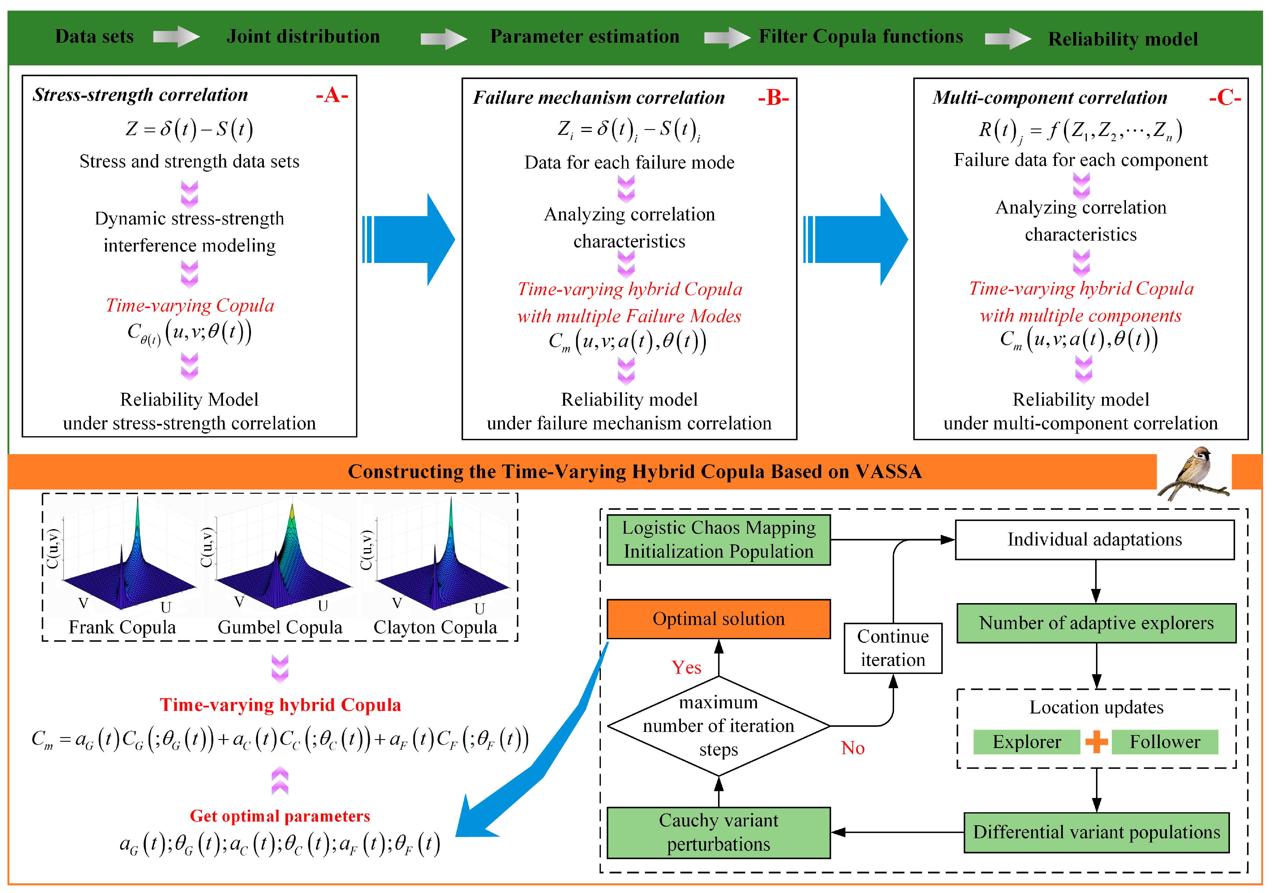
This paper presents a new method for analyzing structural reliability that takes into account the correlation between stress strength, failure mechanism, and multi-components. The implementation process is shown in Figure 1. Firstly, a time-varying Copula [28] is established for a failure mechanism by considering the strength decay and the change in stress–strength correlation with time. This is used to calculate the reliability under a single failure mechanism. A time-varying hybrid Copula is established based on the relevant features of the failure mechanism to calculate the reliability under multiple failure mechanisms. Finally, a time-varying hybrid Copula is constructed to obtain structural reliability for the multi-components.
The method proposed in this paper has the following innovations: (1) to improve the establishment of the reliability model, multiple correlation features are incorporated into the solution process of structural reliability. (2) A time-varying hybrid Copula is established by portraying the time-varying correlation parameter, which accurately characterizes the correlation change law over time and obtains a more accurate analysis of the structural reliability results. (3) To facilitate more efficient and accurate solving for the unknown parameter in the time-varying hybrid Copula model, the variational adaptive sparrow search algorithm (VASSA) is proposed.
The work is structured as follows: Section 2 details the characteristics of stress–strength correlation, failure mechanism correlation, and component correlation. Section 3 explains the construction process of VASSA and how it was built. In Section 4, the performance of VASSA is validated and the reliability-solving method proposed in this paper is demonstrated to be correct and practical through two examples. Finally, the paper concludes with a summary in Section 5.
2. Reliability Modeling of Mechanical Structures Considering Multiple Correlation Characteristics
Mechanical structures can be affected by random loads and various uncertainty factors, resulting in multiple variables, failure mechanisms, and couplings. The correlation between stress and strength is influenced by factors such as part size, loaded condition, and stress concentration [29,30]. Structural fatigue, corrosion, wear, and other failure mechanisms are strongly correlated. For instance, corrosion is more likely to cause cracks in the structure, which in turn can increase the degree of corrosion. To create a more accurate model of structural reliability, correlations of mechanical structures are divided into stress–strength correlation, mechanism correlation, and component correlation.
2.1. Reliability Analysis Considering Stress–Strength Correlation
Over time, the reliability of a mechanical part decreases as it is used. The dynamic stress–strength interference model, illustrated in Figure 2, takes into account the impact of time on reliability [29]. Thus, the model is supposed to result from a cross-interference between the strength–decay process and the random stress process .
2.1.1. Dynamic Stress–Strength Interference Model
Let be the initial strength of the part and the strength decay process is a stochastic process with a continuous set of states and a continuous set of parameters . The strength satisfies the following conditions:
- (1)
- ;
- (2)
- , that is, is a monotonically decreasing function of time ;
- (3)
- Suppose , , then the conditional distribution function of is
Typically, the strength decay process of a part can be characterized using a Gamma stochastic process or set to [31]. is the decay coefficient. is the residual and . Finite element analysis and experimental or sampling data can fit the parameters that characterize the strength decay process.
Stochastic stress processes are generally considered to be smooth processes in which the statistical characteristics of the stress values do not vary with time [31]. Let the initial stress be , then . The distribution characteristics of is the same as .
- (1)
- ;
- (2)
- , that is, is a constant;
- (3)
- Autocorrelation coefficient .
2.1.2. Reliability Model Based on Time-Varying Copula
Stochastic stress processes cause structural strength to decay, which in turn reduces the structure’s ability to withstand random stresses. Therefore, there is a positive correlation between stress and strength. As explained in Section 2.1.1, strength properties vary over time. Similarly, the correlation parameter between stress and strength also varies over time. Let the correlation structure be
where denotes the joint cumulative distribution function. and are the marginal distribution functions. denotes the parameter of the degree of correlation between stress and strength, is the variation parameter, and is the initial correlation parameter.
At the moment , the dynamic correlation interference reliability of the part is modeled as follows:
where is the density function of and is the density function of . If , the system is in the safe stage. If , the system fails. When , the system is in the limit state.
2.2. Reliability Analysis Considering Correlation of Failure Mechanisms
2.2.1. Failure Mechanism Correlation
Multiple failure mechanisms can significantly impact the reliability of mechanical structures due to the relevance of failure mechanisms. Correlation characteristics between multiple failure mechanisms are apparent due to the same load, working environment, material properties, and structural characteristics [32]. For instance, a structure in good condition with no signs of wear on the surface will be less affected by corrosion. In the structure of severe wear, corrosion is likely to increase and vice versa. It is important to analyze the failure mechanisms and construct a corresponding mechanism model. Assuming that the failure behavior of a structure can be characterized by multiple performance functions with one or more identical components between them or that different failure mechanisms act together to cause the failure, it can be determined that the reliability is affected by the correlation of failure mechanisms (as shown in Figure 3).
2.2.2. Reliability Model Based on Time-Varying Hybrid Copula
If a mechanical part has failure mechanisms, according to the change in part strength decay with working time, the distribution of each mode failure life is obtained from the strength decay model. If the correlation structure of is , then the reliability of the part at the moment t is
where is the corresponding ith failure mechanism. is the probability that the part will have the ith failure mechanism before the moment . The “” symbol denotes the differential operation.
To construct failure mechanism correlations, Copula was chosen for its objectivity and to avoid singularity. The characterization scope of Copula was expanded on the relevant structures, resulting in a hybrid Copula. The Gumbel Copula effectively describes upper tail correlation features without affecting lower tail correlation features. The Clayton Copula demonstrates robust lower tail correlation features without affecting overall upper tail correlations [26,33]. The Frank Copula can balance the imbalance in the upper and lower tails of the aforementioned Copulas while providing an accurate representation of correlation features in the intermediate portion [34]. It is important to note that the three Copulas differ in their emphasis on the representation of correlation structures. A time-varying hybrid Copula is constructed using these three Copulas as a foundation. Initially, this study considers the time-varying parameters of the correlation structures. Three types of time-varying Copulas are established based on the description in Section 2.1. Subsequently, a time-varying hybrid Copula is constructed to ensure a complete and rational description of the correlation in the failure mechanism. The time-varying hybrid Copula can be expressed as
where , , and are the weight coefficients of the three Copula of Gumbel, Clayton, and Frank, respectively, all of which are time-varying and . , , and are the time-varying correlation parameters of the three Copula. Using Equation (5) instead of the correlation structure in Equation (4) for calculation, the reliability of the part under the correlation of failure mechanism can be obtained.
Equation (5) reveals that the time-varying hybrid Copula has six unknown parameters. The structure of the time-varying hybrid Copula, the edge distribution of each failure mechanism, and the correlation degree parameter between the failure mechanisms are all time-varying. This presents a significant challenge for evaluating and solving the time-varying hybrid Copula. In this complex computational environment, accurately determining the parameters of the time-varying hybrid Copula is crucial. The auto-regressive moving average model (ARMA) is an essential method for time series analysis, which can obtain the time-varying parameters of the hybrid Copula [35]. Constructing the time-varying hybrid Copula model requires calculating the correlation structure and performance function at each moment, making it computationally intensive to solve using ARMA. To address this issue, this paper proposes using the variational adaptive sparrow search algorithm (VASSA) to obtain the values of unknown parameters in the hybrid model.
2.3. Reliability Analysis under Multi-Component Correlation
Mechanical systems typically consist of multiple components that work together to achieve the system’s function. As a result, the components are positively correlated. However, since each component has a distinct function, there is no deterministic correlation structure between them, making it difficult to quantify the correlation. Section 2.2 uses a time-varying hybrid Copula to characterize the correlation structure between multiple components effectively. The failure data of each component were analyzed to assess the degree of correlation between them. Subsequently, a structural reliability model was established, taking into account the multi-component correlation characteristics, as per Equation (5). Finally, the reliability of the mechanical mechanism was determined, considering the triple correlation characteristics.
2.4. Reliability-Solving Process under Multiple Correlation Characteristics
Step 1: The structural strength’s stochastic degradation is calculated using the Gamma stochastic process, based on its changing characteristics over time. This can be expressed as
where is the Gamma stochastic process. and are the expectation and variance, respectively. The and are the shape function and size parameter coefficients, respectively.
Step 2: Obtain the structural stress dataset and calculate the distributional characteristics.
Step 3: Determine the relevance of the stress–strength dataset using the rank correlation coefficient as a consistency measure. Let the random variable be , if , and are said to be positively correlated. Conversely, and are negatively correlated. The commonly used Kendall rank correlation coefficient is
Step 4: The objective of this task is to determine the appropriate Copula choice, construct the corresponding time-varying Copula and test its goodness of fit using the statistical squared difference method.
Step 5: Calculate the reliability data under each failure mechanism according to Equation (3).
Step 6: Analyze the correlation structure between the failure mechanisms and construct the time-varying hybrid Copula based on the reliability data of each failure mechanism and Equation (5).
Step 7: To complete the reliability model in multiple failure mechanisms, solve the unknown parameters of the time-varying hybrid Copula using VASSA and assess the goodness-of-fit using the Akaike information criterion.
Step 8: Analyze the correlation structure between components and calculate the time-varying hybrid Copula between multiple components. Then, follow the steps in the sixth and seventh sections to determine the reliability of the mechanical structure.
3. Variational Adaptive Sparrow Search Algorithm-VASSA
The sparrow search algorithm (SSA) is a novel population intelligence optimization algorithm based on sparrow foraging and anti-predator behaviors [36]. The bionic principle of the SSA is to divide the foraging sparrows into explorers and joiners and introduce an early warning mechanism. SSA has the advantages of easy expansion, good self-organization, and robustness. The explorer searches a wide range and guides the population search, while the joiners follow the explorer in searching for better adaptation. Joiners may monitor the explorer to search for food or compete for it, seeking better adaptation. If the entire population is at risk, an early warning agent will signal danger and the colony will engage in anti-predatory behavior, abandoning the current food source and moving to a safe location. As the population intelligence optimization algorithm approaches the global optimum, population diversity decreases, making it easier to fall into a local optimum. To enhance search accuracy and convergence speed, this paper proposes improvements to the SSA due to the issues mentioned above.
3.1. Initializing Populations Based on Logistic Chaos Mapping
Chaotic motion is a type of random dynamic motion that offers the benefits of randomness and traversal. When computing the optimal solution problem of a function, the advantages of chaotic motion can make the algorithm more likely to escape local optimal solutions and improve the exploration ability while ensuring population diversity. The use of logistic chaos mapping results in a population that is more dispersed and uniform compared to a randomly generated population, which in turn accelerates the convergence speed of the algorithm [37]. The mathematical expression for logistic chaos mapping is
where is the position of the ith individual in the dth dimensional space. is the upper limit in the dth dimensional space. is the lower limit in the dth dimensional space. is the chaos parameter of the ith sparrow in the dth dimensional space.
3.2. Adaptive Number of Individual Explorers and Improved Explorer Position Update Formulae
The original algorithmic mechanism may cause some joiners to search following the explorer but this search capability is limited. To enable the algorithm to transition from global to local search as quickly as possible in later stages, we propose using the adaptive explorer number model instead of the original explorer model. The expression for the adaptive explorer number model is
where is the number of populations and is the number of explorers. t is the number of current iterations and is the maximum number of iterations. In the early stage of the algorithm, the number of explorers is kept at N/2, aiming to keep the algorithm efficient in global exploration and make the search region more traversable. When the number of optimization iterations is halfway through, the number of explorers is gradually reduced to speed up the algorithm’s convergence to perform local search as soon as possible.
In addition, the original algorithm’s formula for updating explorer positions was changed to [18]
where is a uniform random number between (0, 1]. is a random number obeying a standard normal distribution and denotes a matrix of size 1 × d with elements all 1. ∈ [0, 1] and ∈ [0.5, 1] denote the warning value and the safety value, respectively, with denoting safety and denoting the presence of a predator. m is a random number between [1, 4].
3.3. Differential Variant Populations
The study randomly selects two individuals from the sparrow population and calculates the distance between them. The to-be-mutated individual of the joiner undergoes a vector summation operation using the scale factor and the position of the current optimal solution. In this paper, we choose the mutation method of DE/rand-to-best/1/bin and the expression of the position update of the individual to be mutated is
where is a random number between 0 and 1, this paper takes 0.35. and are both random numbers between 0 and 1. denotes the current global optimal solution. denotes the variation scale factor, balancing the global search and local development. When F is large, the global search for optimality is carried out but the convergence efficiency of the algorithm will be sacrificed. However, when F is minor, although the convergence efficiency can be guaranteed, it takes work to jump out of the local optimality search region. To balance the above problems, this paper introduces a linearly varying variational scale factor, whose expression is
where is the upper limit of the scale factor and is the lower limit of the scale factor.
3.4. Optimal Solutions for Cauchy’s Variational Perturbations
If the algorithm converges too fast, the results converge to the local optimal solution. This paper introduces Cauchy variation for the stochastic optimal solution to jump out of the local optimal solution [38]. The expression of the Cauchy variation is
where is the optimal solution after mutation perturbation and is Cauchy’s coefficient of variation.
In summary, the flow of solving the unknown parameters of the hybrid Copula model using the variational adaptive sparrow search algorithm is shown in Figure 4.
4. Case Study and Validation
4.1. Performance Validation of VASSA
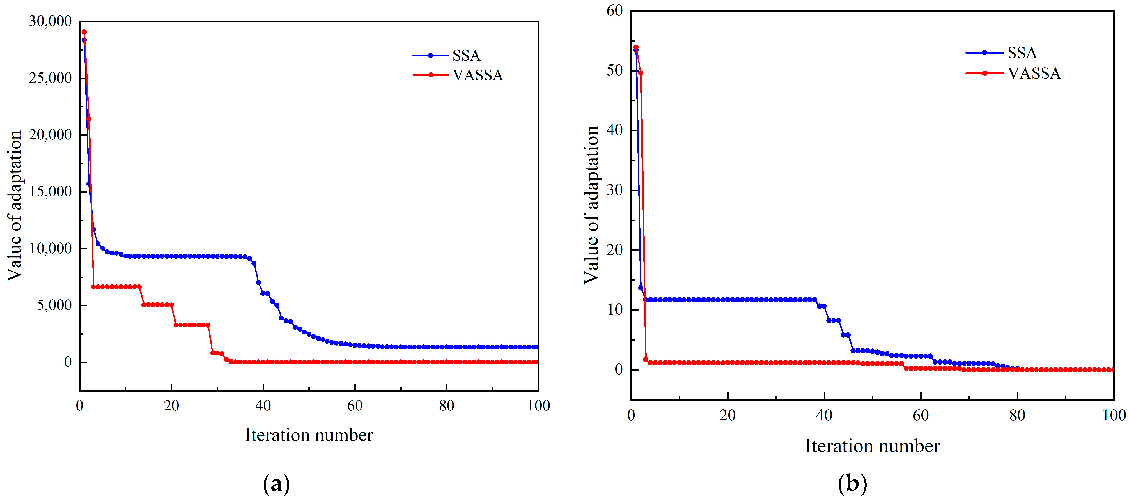
The performance of VASSA was evaluated using the Sphere and Griewank functions. The algorithm’s population size was set to 30 and the number of iterations was set to 100. The convergence curve is shown in Figure 5.
Figure 5 shows that VASSA outperforms the original SSA in terms of convergence speed and computational accuracy for the two test functions. To provide a quantitative description of the advantages of the improved algorithms, both algorithms were used to compute the two functions 50 times. Table 1 displays the optimal solution, worst solution, standard deviation, and mean value of the computed results.
Table 1 shows that VASSA achieves significantly higher solution accuracies for the Sphere function compared to SSA. The optimal solution, worst solution, and mean value of VASSA are improved by 40, 10, and 12 orders of magnitude, respectively. Additionally, VASSA exhibits better robustness as evidenced by the 10 orders of magnitude improvement in standard deviation solution accuracy. The Griewank function analysis shows that VASSA achieves the true optimal solution. Additionally, the solution accuracy and robustness of VASSA are superior to the original SSA. Therefore, VASSA is a better option for solving the unknown parameters of the time-varying hybrid Copula function.
4.2. Verification of Structural Reliability Calculation Methods under Multiple Correlation Features
4.2.1. Case 1: Connecting Rod Mechanism
Following the logic flow in Figure 1, the stress and strength correlations are first analyzed, then the failure mechanism correlations are calculated and finally, the correlation characteristics between multiple components are calculated. In Case 1, there are two failure components: connecting rod CE and joint D. Among them, connecting rod CE has two failure mechanisms. In Case 2, there are three failure components: gear, bearing inner ring, and bearing outer ring. The gear has two modes of failure, while the inner and outer rings of the bearing are only involved in the analysis and calculation of stress–strength correlation and multi-component correlation characteristics.
Figure 6 shows a simplified version of the kinematic mechanism of the connecting rod. The reliability of this mechanism’s motion is mainly affected by the torsional deformation of the rods and the wear of the rotating joints. The main failures are torsional and fatigue strength failures of the connecting rod CE and wear failures of the joint D. Table 2 presents the stress and strength data for each failure.
It is assumed that both strength and stress obey normal distribution and the coefficient of variation is taken as 0.001. In this case, the strength conforms to the linear decay model with a degradation rate of 0.02. The reliabilities of the kinematic structure of the connecting rod in each failure mechanism are calculated separately, as shown in Figure 7. In Figure 7, denotes the reliability of the rotating joint D under wear failure mechanism and and are the reliabilities of the rod CE under fatigue failure and torsion failure, respectively.
The reliability curves show a faster-decreasing trend when considering the stress–strength correlation feature. For the wear failure mechanism of the rotating joint D and the torsional failure mechanism of the bar CE, the reliabilities and are more significant when considering the stress–strength correlation at the early stage. At a later stage, reliabilities that take into account stress–strength correlation are smaller than those without correlation. In terms of the fatigue failure mechanism of bar CE, reliability is always smaller when considering the stress–strength correlation than when not considering it. During the pre-service period, the correlation parameter undergoes minimal change, resulting in a small decay degree of strength for each mode. Therefore, reliability is more significant when considering the stress–strength correlation feature than when not considering it. However, over time, the correlation degree parameter becomes increasingly prominent. Therefore, the reliability of considering the stress–strength correlation feature decreases more than that of not considering the correlation feature. In conclusion, the stress–strength correlation cannot be ignored in the structural reliability analysis.
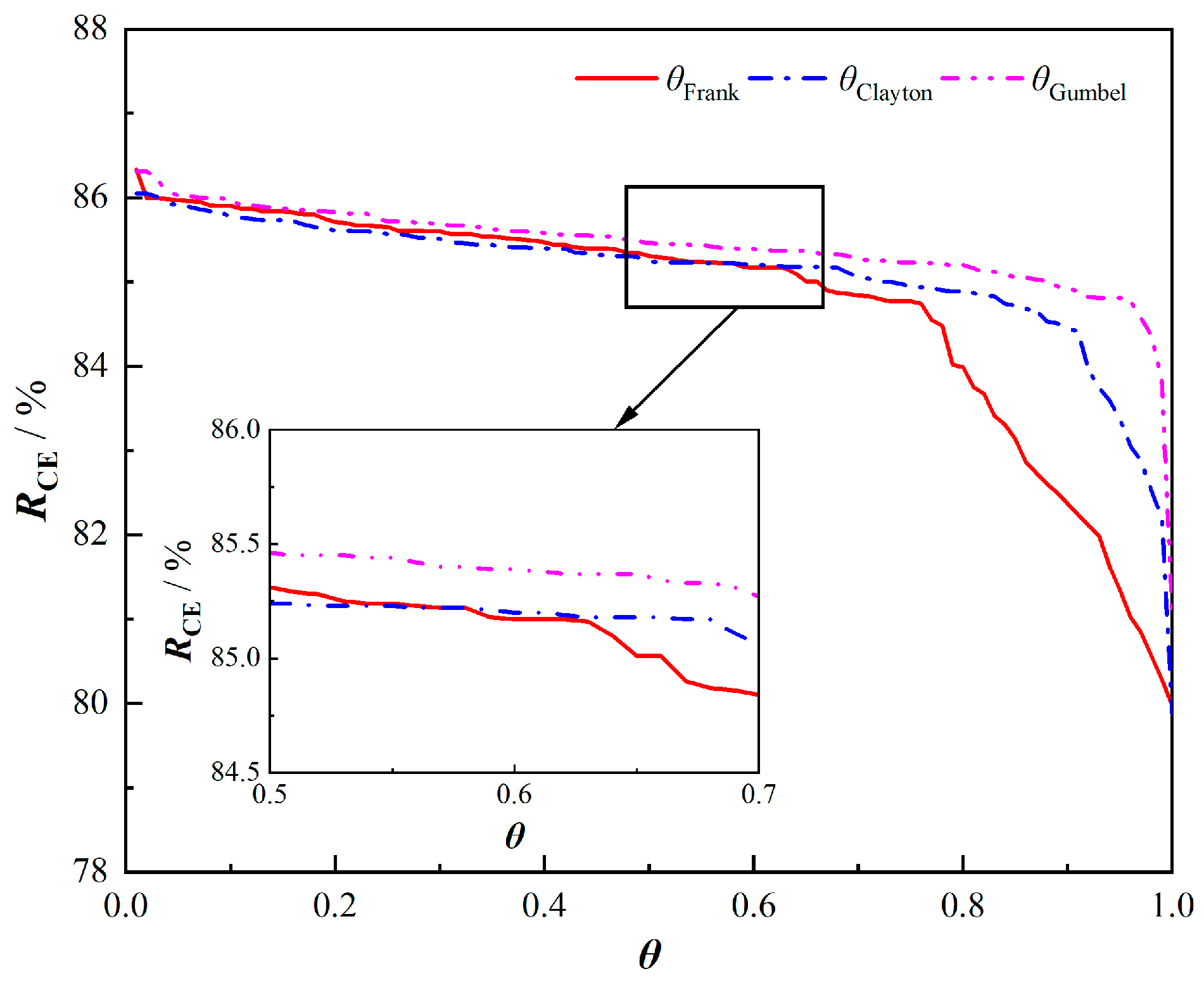
The two failure mechanisms of rod CE are in the same service environment and there is a complex relationship between them in which they interact and compete. Three Copula of Frank, Gumbel, and Clayton are selected to construct the time-varying hybrid Copula. Firstly, the influence of the correlation parameters in the three Copula on the reliability of the bar CE needs to be explored and the results are shown in Figure 8.
Figure 8 shows that the parameter for the correlation degree of the Frank Copula has the greatest impact on the structural reliability described by the time-varying hybrid Copula, followed by the Clayton Copula correlation degree parameter. The Gumbel Copula correlation degree parameter has the least impact. Meanwhile, it is important to note that when the correlation degree parameter reaches a certain size, the reliability decreases significantly. This suggests that the deviation of the time-varying hybrid Copula in calculating structural reliability increases. Therefore, it is recommended to limit the selection of the three Copula within a specific range. VASSA is used to estimate the parameters of the time-varying hybrid Copula, which characterizes the correlation between the two failure mechanisms of the bar CE. The reliability of the bar CE is then determined.
where , , and .
The reliabilities of the bar CE considering the failure mechanism correlation and a single failure mechanism are given in Figure 9. It can be seen that the reliability of the bar CE considering the stress–strength correlation and the failure mechanism correlation is lower than that in either of the independent failure mechanisms. This result proves that the effect of multilevel correlation on the time-varying reliability cannot be neglected. Otherwise, the reliability will be overestimated, which will cause safety hazards. The phase of service in the independent failure mechanism is difficult to define, especially in the middle of service, where reliability does not level off but declines rapidly. After considering the correlation of failure mechanisms, three stages are evident from the reliability curves: infant mortality stage, random failure stage, and wear-out stage. The results show that when a component has multiple failure mechanisms, it is necessary to consider the correlation of failure mechanisms and the reliability calculated from this is more scientific and relevant to reality.
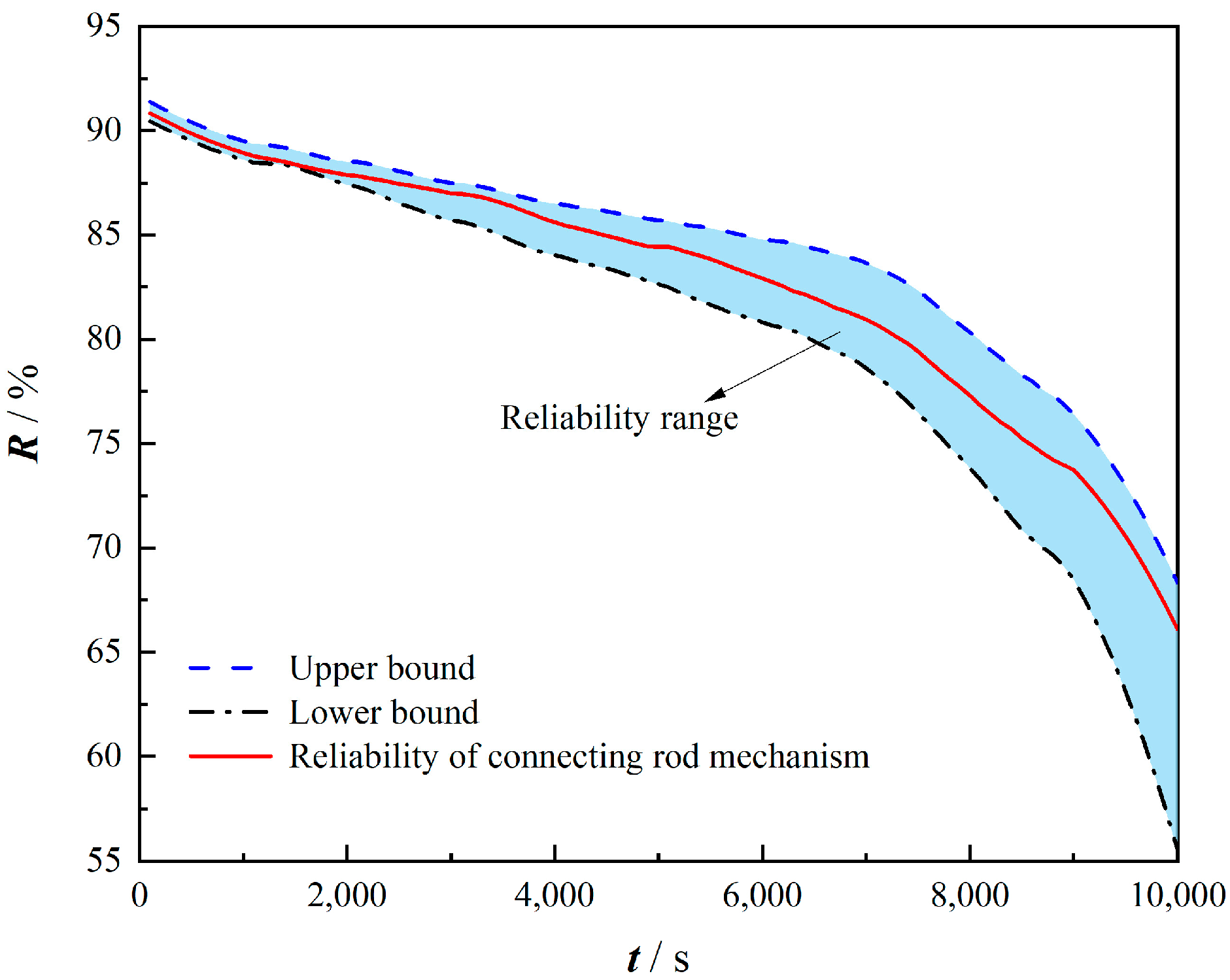
Based on single-part reliability analysis, the reliability of the linkage mechanism calculated by considering the correlation between multiple parts is shown in Figure 10. The traditional method primarily calculates the reliability range of a complex system in series. It considers that the system reliability should be in the interval with the product of the minimum reliability of parts and the reliability of all parts as the endpoint, that is, the upper and lower limits of the reliability interval. As can be seen from Figure 10, the reliability of the connecting rod mechanism is always within the range of the reliability calculated by the traditional method, which proves the correctness and robustness of this paper’s method. The reliability of the mechanical structure can be calculated very accurately by considering the stress–strength correlation, the failure mechanism correlation, and the component correlation.
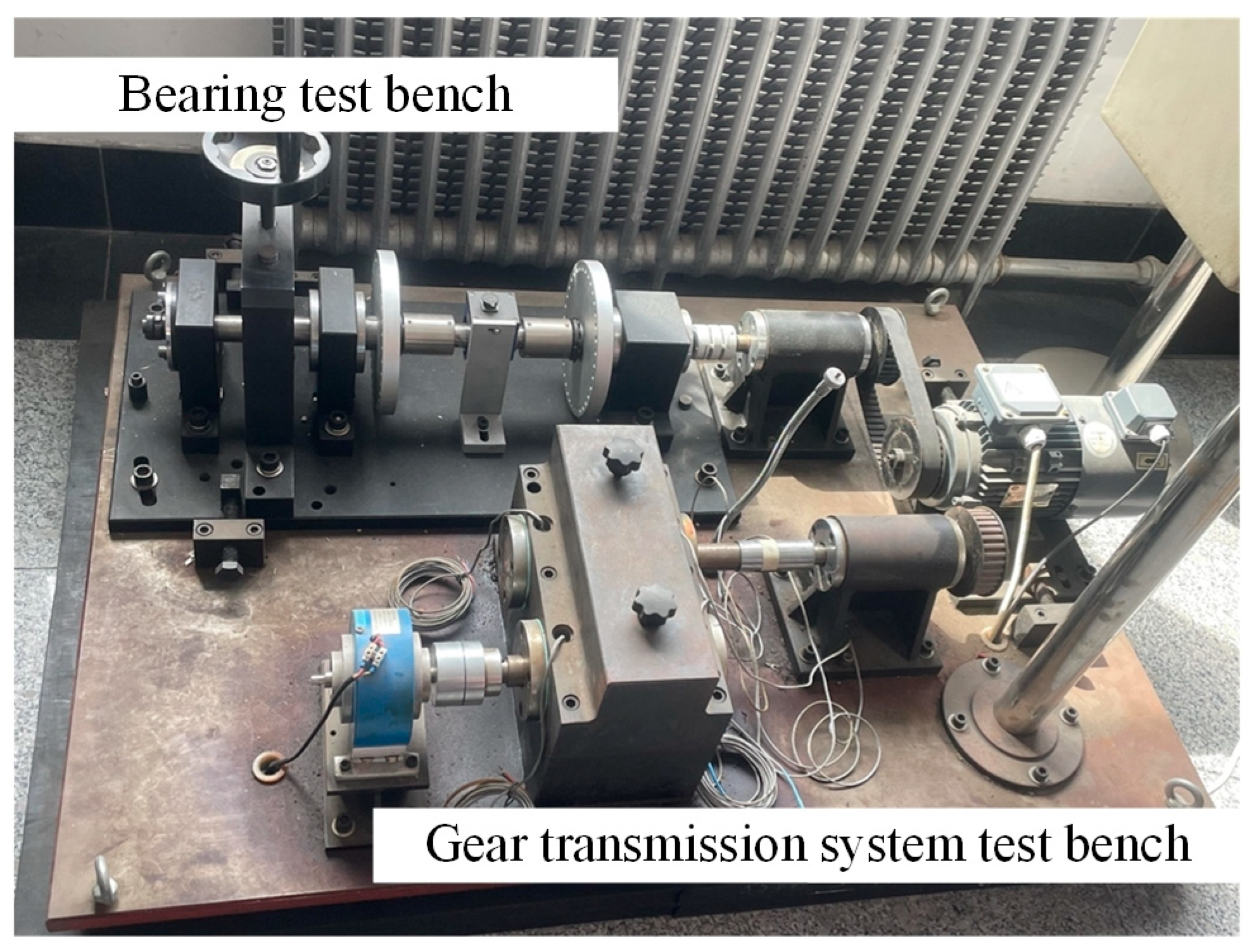
4.2.2. Case 2: Gear Transmission System
The gear train equipment is shown in Figure 11. Gear failure forms are mainly tooth surface wear and root cracks. Bearing failure is mainly fatigue failure of the inner ring and outer ring. The gear wear and crack data are tested in the gear transmission test rig and then the faulty bearing is disassembled and put into the bearing test rig to detect the vibration signal. The vibration signal is used as the bearing failure data. The gear and bearing test results are obtained, as shown in Figure 12.
Tooth wear test data are given in Figure 12a, root crack test data are given in Figure 12b, and Figure 12c shows the frequency domain diagram of vibration signals of the inner and outer rings of the bearing. In the same service environment, pinion gears are more prone to wear than larger gears. Therefore, only the pinion gear is measured for wear. The calculation and distribution of gear wear are shown in Figure 12a. The mean and standard deviation of the maximum wear amount of different gear teeth are counted and the wear failure threshold is reasonably assumed according to the literature. Calculate the mean value and standard deviation of the crack expansion rate. Based on engineering experience, it can be determined that the crack expansion rate is generally in the range of 1 × 10⁻⁹~1 × 10⁻⁵ and this paper selects 1 × 10⁻⁵ as the crack expansion failure threshold. In addition, when the crack expands to the gear tooth axis, the gear is judged to fail. The expansion rates of the three tooth root cracks are shown in Figure 12b. Bearing failure is usually diagnosed on the basis of vibration frequency as established in this paper as well as the bearing vibration signals collected from experimental tests to assess whether the bearings are failing or not. The vibration frequencies of the inner and outer rings of the bearing are shown in Figure 12c. The final statistics obtained the data distribution characteristics in Table 3.
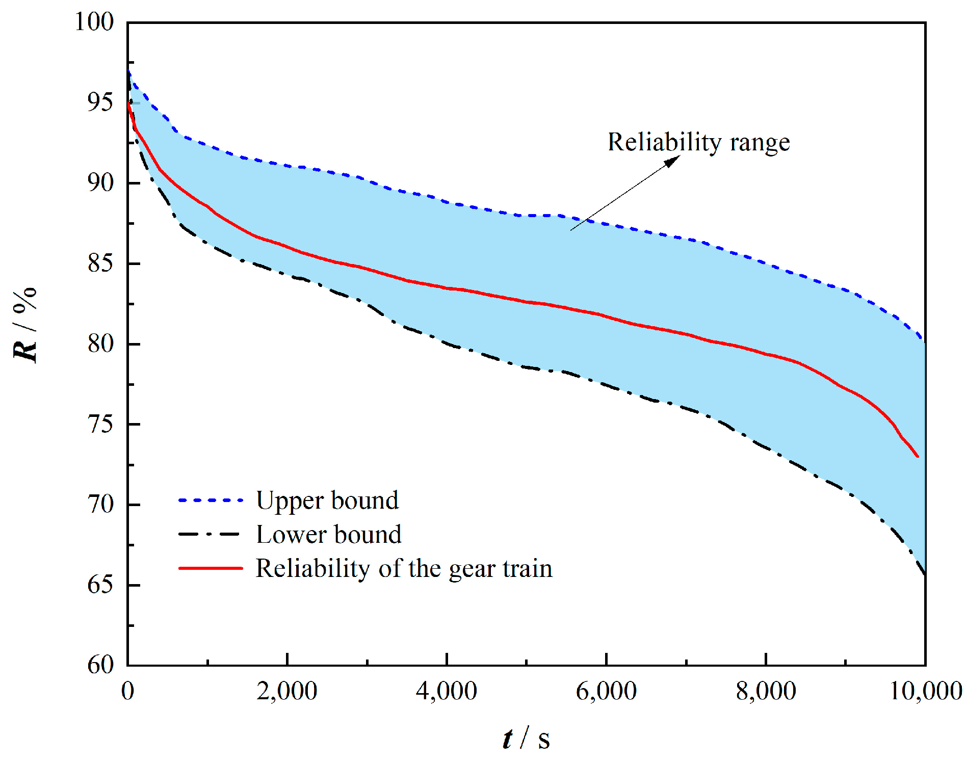
Based on the test data, the reliability analysis of the gear transmission system under the action of multiple relevant features is carried out. Figure 13 shows the reliability of gears and bearings in each failure mechanism under the stress–strength correlation structure, Figure 14 shows the reliability of gears under the correlation of failure mechanism and the reliability of bearings under the correlation of components, and Figure 15 shows the results of the reliability of the gear transmission system.
As shown in Figure 13, the reliability of both gears and bearings decreases after considering the stress–strength correlation feature. The decreasing trend of reliability after considering stress–strength correlation is greater than the decreasing trend before considering it. From Figure 13a, it can be seen that tooth face wear has a more significant effect on the time-varying reliability of gears compared to root cracks. Tooth flank wear is unavoidable during meshing and gradually increases with the increase in meshing cycles. The emergence and expansion of cracks have a strong chance and randomness. Although this paper prefabricated the initial crack of 0.27 mm in the specimen, the relationship between the crack expansion rate and the meshing cycle has a strong randomness. In Figure 13b, the reliabilities of the inner and outer rings of the bearings under the stress–strength correlation feature are overall lower than those without considering the stress–strength correlation and this result again proves that the stress–strength correlation has an enormous influence on the reliability.
Figure 14 shows a positive correlation between tooth surface wear and root crack, as well as between the bearing inner ring and outer ring. This means that a failure mechanism or component failure can worsen the failure process of another mode or component. Figure 14a illustrates that tooth surface wear and tooth root crack interact, exacerbating the gear failure process. Reliability under a single failure mechanism is overly optimistic and does not accurately reflect the actual reliability of the gear during operation. Figure 14b demonstrates the impact of multi-component correlation features on reliability, which is similar to the influence of failure mechanism correlation. The reliability of a bearing represented by either the inner or outer ring alone is higher than the reliability of the bearing when considering the correlation of components. Failure mechanisms and correlation characteristics between multiple components must be considered to avoid overestimating the reliability of the gear train. This is important for maintenance optimization and feedback design.
The reliability of the gear transmission system is determined by considering the relevant failure characteristics between gears and bearings, as shown in Figure 15. The upper limit of reliability is the minimum value of reliability of gears and bearings at the same moment and the lower limit is the reliability of gears and bearings in series connection. The reliability of the gearing system calculated by the method presented in this paper consistently falls within the range of reliability calculated by the reliability limit theory. This result demonstrates the accuracy and stability of the method. Compared to reliability calculation results based on the assumption of independence, the reliability results calculated using the method proposed in this paper, which considers various related features, are more realistic and aligned with engineering reality.
5. Conclusions
This paper proposes a new method for structural reliability analysis that considers the stress–strength correlation, failure mechanism correlation, and multi-component correlation. The method has been proven to be reliable and the calculation results are more in line with engineering reality, as demonstrated through example analysis. In reliability analysis of mechanical mechanisms, failure to consider correlation characteristics or only considering a single correlation can lead to overestimation of structural reliability, which can result in safety hazards.
- (1)
- Compared to the reliability calculation results based on the independence assumption, the reliability results obtained by considering various related features clearly demonstrate the different service stages. This proves that the method’s calculation results align with the pre-estimation of the bathtub curves, avoiding the pitfalls caused by overestimating reliability. Consequently, it is beneficial for the operation and optimization of the design;
- (2)
- After exploring various correlation structures, this study proposes the time-varying hybrid Copula by combining three different Copula models: Gumbel, Frank, and Clayton. The results of the example validation demonstrate that the time-varying hybrid Copula effectively characterizes the variation of time-varying parameters of the correlation structures. Frank Copula has the most significant influence on the characterization ability of the time-varying hybrid Copula, while Gumbel Copula has the most negligible influence;
- (3)
- The time-varying characteristics of relevant parameters and uncertain parameters of the hybrid Copula, along with the intensity decay process, make it computationally intensive and challenging to compute the optimal values of the unknown parameters of the time-varying hybrid Copula. Therefore, this paper proposes VASSA, which is verified using the Sphere and Griewank functions. The results demonstrate that VASSA achieves significantly higher accuracy in solving optimal, worst, and mean value solutions compared to SSA, by more than 10 orders of magnitude. VASSA exhibits good stability, solution accuracy, and speed.
Author Contributions
Conceptualization, X.B.; methodology, X.B. and Y.L.; software, X.B. and D.Z.; validation, X.B.; data curation, Z.Z.; writing—original draft preparation, X.B.; writing—review and editing, X.B. and Y.L.; visualization, X.B., D.Z. and Z.Z.; supervision, Y.L.; project administration, Y.L. All authors have read and agreed to the published version of the manuscript.
Funding
This research was funded by the National Natural Science Foundation of China, grant number 51875073, and the Science and Technology Innovation Project of Liaoning Provincial Department of Education, grant number JYTMS20230002.
Data Availability Statement
The data that support the findings of this study are available from the corresponding author upon reasonable request.
Conflicts of Interest
The authors declare no conflicts of interest.
References
- Chen, J.; Feng, Y.; Teng, D.; Lu, C.; Fei, C. Selective transmit modeling framework of complex system reliability analysis considering failure correlation. Eng. Fail. Anal. 2024, 158, 107957. [Google Scholar] [CrossRef]
- Jafary, B.; Mele, A.; Fiondella, L. Component-based system reliability subject to positive and negative. Reliab. Eng. Syst. Saf. 2020, 202, 107058. [Google Scholar] [CrossRef]
- Eem, S.; Kwag, S.; Choi, I.; Hahm, D. Sensitivity analysis of failure correlation between structures, systems, and components on system risk. Nucl. Eng. Technol. 2023, 55, 981–988. [Google Scholar] [CrossRef]
- Wang, Y.; Xie, M.; Su, C. Multi-objective maintenance strategy for corroded pipelines considering the correlation of different failure modes. Reliab. Eng. Syst. Saf. 2024, 243, 109894. [Google Scholar] [CrossRef]
- Akgül, F.G.; Acitas, S.; Senoglu, B. Inferences on stress–strength reliability based on ranked set sampling data in case of Lindley distribution. J. Stat. Comput. Sim. 2018, 88, 3018–3032. [Google Scholar] [CrossRef]
- James, A.; Chandra, N.; Sebastian, N. Stress-strength reliability estimation for bivariate copula function with Rayleigh marginals. Int. J. Syst. Assur. Eng. Manag. 2023, 14, S196–S251. [Google Scholar] [CrossRef]
- Adumene, S.; Khan, F.; Adedigba, S.; Zendehboudi, S. Offshore system safety and reliability considering microbial influenced multiple failure modes and their interdependencies. Reliab. Eng. Syst. Saf. 2021, 215, 107862. [Google Scholar] [CrossRef]
- Cho, S.E. First-order reliability analysis of slope considering multiple failure modes. Eng. Geol. 2013, 154, 98–105. [Google Scholar] [CrossRef]
- Liu, N.; Hu, M.; Wang, J.; Ren, Y.; Tian, W. Fault detection and diagnosis using Bayesian network model combining mechanism correlation analysis and process data: Application to unmonitored root cause variables type faults. Process Saf. Environ. 2022, 164, 15–29. [Google Scholar] [CrossRef]
- Li, X.; Song, L.; Bai, G. Failure correlation evaluation for complex structural systems with cascaded synchronous regression. Eng. Fail. Anal. 2022, 141, 106687. [Google Scholar] [CrossRef]
- Low, B.K.; Zhang, J.; Wilson, H. Tang. Efficient system reliability analysis illustrated for a retaining wall and a soil slope. Comput. Geotech. 2011, 38, 196–204. [Google Scholar] [CrossRef]
- Ghosh, S.; Bhattacharya, B. A nested hierarchy of second order upper bounds on system failure probability. Probabilist. Eng. Mech. 2022, 70, 103335. [Google Scholar] [CrossRef]
- Liu, X.; Li, T.; Zhou, Z.; Hu, L. An efficient multi-objective reliability-based design optimization method for structure based on probability and interval hybrid model. Comput. Method. Appl. M. 2022, 392, 114682. [Google Scholar] [CrossRef]
- Ajenjo, A.; Ardillon, E.; Chabridon, V.; Iooss, B.; Cogan, S.; Sadoulet-Reboul, E. An info-gap framework for robustness assessment of epistemic uncertainty models in hybrid structural reliability analysis. Struct. Saf. 2022, 96, 102196. [Google Scholar] [CrossRef]
- Gerasimov, A.; Vorechovsky, M. Failure probability estimation and detection of failure surfaces via adaptive sequential decomposition of the design domain. Struct. Saf. 2023, 104, 102364. [Google Scholar] [CrossRef]
- Li, G.; Wang, D.; Wang, K.; Lin, L. A two-dimensional sample screening method based on data quality and variable correlation. Anal. Chim. Acta 2022, 1203, 339700. [Google Scholar] [CrossRef]
- Lima, J.P.; Evangelista, F., Jr.; Soares, C.G. Bi-fidelity Kriging model for reliability analysis of the ultimate strength of stiffened panels. Mar. Struct. 2023, 91, 103464. [Google Scholar] [CrossRef]
- Tian, Z.; Zhi, P.; Guan, Y.; Feng, J.; Zhao, Y. An effective single loop Kriging surrogate method combing sequential stratified sampling for structural time-dependent reliability analysis. Structures 2023, 53, 1215–1224. [Google Scholar] [CrossRef]
- Leite, M.; Costa, M.A.; Alves, T.; Infante, V.; Andrade, A.R. Reliability and availability assessment of railway locomotive bogies under correlated failures. Eng. Fail. Anal. 2022, 135, 106104. [Google Scholar] [CrossRef]
- Diana, T. Improving schedule reliability based on copulas: An application to five of the most congested US airports. Aerosp. Sci. Technol. 2011, 17, 284–287. [Google Scholar] [CrossRef]
- Liu, L.; Xu, Y.; Zhu, W.; Zhang, J. Effect of copula dependence structure on the failure modes of slopes in spatially variable soils. Comput. Geotech. 2024, 166, 105959. [Google Scholar] [CrossRef]
- Zhao, Y.; Dong, S. Multivariate probability analysis of wind-wave actions on offshore wind turbine via copula-based analysis. Ocean Eng. 2023, 288, 116071. [Google Scholar] [CrossRef]
- Nabizadeh, F.C.; Valikhan, M.A.; Mahmoudian, F.; Farzin, S. A new methodology for the prediction of optimal conditions for dyes’ electrochemical removal; Application of copula function, machine learning, deep learning, and multi-objective optimization. Process. Saf. Environ. 2024, 182, 298–313. [Google Scholar] [CrossRef]
- Messoudi, S.; Destercke, S.; Rousseau, S. Copula-based conformal prediction for multi-target regression. Pattern Recogn. 2021, 120, 108101. [Google Scholar] [CrossRef]
- Bekdemir, L.; Bazlamaçcı Cüneyt, F. Hybrid probabilistic timing analysis with Extreme Value Theory and Copulas. Microprocess. Microsy. 2022, 89, 104419. [Google Scholar] [CrossRef]
- Schinke-Nendza, A.; Von Loeper, F.; Osinski, P.; Schaumann, P.; Schmidt, V.; Weber, C. Probabilistic forecasting of photovoltaic power supply—A hybrid approach using D-vine copulas to model spatial dependencies. Appl. Energy 2021, 304, 117599. [Google Scholar] [CrossRef]
- Arrieta-Prieto, M.; Schell Kristen, R. Spatio-temporal probabilistic forecasting of wind power for multiple farms: A copula-based hybrid model. Int. J. Forecast. 2022, 38, 300–320. [Google Scholar] [CrossRef]
- Ma, P.; Zhang, Y. A time-varying copula approach for describing seasonality in multivariate ocean data. Mar. Struct. 2024, 94, 103567. [Google Scholar] [CrossRef]
- Ye, K.; Wang, H.; Ma, X. A generalized dynamic stress-strength interference model under δ-failure criterion for self-healing protective structure. Reliab. Eng. Syst. Saf. 2023, 229, 108838. [Google Scholar] [CrossRef]
- Qian, H.; Li, Y.; Huang, H. Time-variant system reliability analysis method for a small failure probability problem. Reliab. Eng. Syst. Saf. 2021, 205, 107261. [Google Scholar] [CrossRef]
- Woloszyk, K.; Goerlandt, F.; Montewka, J. A methodology for ultimate strength assessment of ship hull girder accounting for enhanced corrosion degradation modelling. Mar. Struct. 2024, 93, 103530. [Google Scholar] [CrossRef]
- Tandel, R.R.; Patel, R.N.; Jain, S.V. Correlation development of erosive wear and silt erosion failure mechanisms for pump as turbine. Eng. Fail. Anal. 2023, 153, 107610. [Google Scholar] [CrossRef]
- Xu, M.; Herrmann, J.W.; Droguett, E.L. Modeling dependent series systems with q-Weibull distribution and Clayton copula. Appl. Math. Model. 2021, 94, 117–138. [Google Scholar] [CrossRef]
- De Baets, B.; De Meyer, H. Cutting levels of the winning probability relation of random variables pairwisely coupled by a same Frank copula. Int. J. Approx. Reason. 2019, 112, 22–36. [Google Scholar] [CrossRef]
- Castiglione, J.; Astroza, R.; Azam, S.E.; Linzell, D. Auto-regressive model based input and parameter estimation for nonlinear finite element models. Mech. Syst. Signal Pr. 2020, 143, 106779. [Google Scholar] [CrossRef]
- Li, J.; Chen, J.; Shi, J. Evaluation of new sparrow search algorithms with sequential fusion of improvement strategies. Comput. Ind. Eng. 2023, 182, 109425. [Google Scholar] [CrossRef]
- Da Costa, D.R.; Medrano-T, R.O.; Leonel, E.D. Route to chaos and some properties in the boundary crisis of a generalized logistic mapping. Phys. A 2017, 486, 674–680. [Google Scholar] [CrossRef]
- Akash, M.; Prashanth, L.A.; Shalabh, B. Truncated Cauchy random perturbations for smoothed functional-based stochastic optimization. Automatica 2024, 162, 111528. [Google Scholar] [CrossRef]
Figure 1.
Schemes follow the same formatting.

Figure 2.
Interference modeling of dynamic stress–strength correlations.

Figure 3.
Schematic of the correlation of the failure mechanism.

Figure 4.
Flowchart of construction of hybrid Copula function based on VASSA.

Figure 5.
Schemes follow the same formatting: (a) Iteration curve of the sphere function; (b) Iteration curve of the Griewank function.
Figure 5.
Schemes follow the same formatting: (a) Iteration curve of the sphere function; (b) Iteration curve of the Griewank function.

Figure 6.
Connecting rod mechanism motion diagram.

Figure 7.
Reliability in each failure mechanism.

Figure 8.
Influence of the correlation degree parameter on the reliability of rod CE.

Figure 9.
Reliability of rod CE.

Figure 10.
Reliability of the connecting rod mechanism.

Figure 11.
Troubleshooting test bed for gear transmission systems.

Figure 12.
Test data for each failure mechanism of the gear train: (a) wear of tooth surface; (b) tooth root crack; and (c) frequency domain diagram of bearing vibration.
Figure 12.
Test data for each failure mechanism of the gear train: (a) wear of tooth surface; (b) tooth root crack; and (c) frequency domain diagram of bearing vibration.


Figure 13.
Reliability of gear and bearing under stress–strength correlation: (a) reliability of the gear and (b) reliability of the bearing.
Figure 13.
Reliability of gear and bearing under stress–strength correlation: (a) reliability of the gear and (b) reliability of the bearing.

Figure 14.
Reliability of gears and bearings in different relevant configurations: (a) reliability of gears and bearings in different relevant configurations and (b) reliability of bearing under multi-component correlation.
Figure 14.
Reliability of gears and bearings in different relevant configurations: (a) reliability of gears and bearings in different relevant configurations and (b) reliability of bearing under multi-component correlation.

Figure 15.
Reliability of gear transmission system.


Table 1.
Comparison of algorithm calculation results.
| Function Name | Evaluation Metrics | SSA | VASSA |
|---|---|---|---|
| Sphere | Optimal solution | 4.98 × 10² | 3.35 × 10−38 |
| Worst solution | 2.12 × 10³ | 3.02 × 10⁻⁷ | |
| Mean value | 1.45 × 10³ | 6.95 × 10⁻⁹ | |
| Standard deviation | 4.37 × 10² | 4.21 × 10⁻⁸ | |
| Griewank | Optimal solution | 2.01 × 10⁻² | 0.00 |
| Worst solution | 6.43 × 10⁻¹ | 1.02 × 10⁻¹² | |
| Mean value | 2.08 × 10⁻¹ | 2.38 × 10⁻¹⁴ | |
| Standard deviation | 1.54 × 10⁻¹ | 1.77 × 10⁻¹³ |
Table 2.
Parameters of the connecting rod mechanism.
| Parts and Components | Failure Mechanism | Mean | Unit | |
|---|---|---|---|---|
| connecting rod (CE) | torsional | 1.05 × 10⁻² | 0.96 × 10⁻² | N·m/deg |
| fatigue | 235.00 | 217.00 | Mpa | |
| revolute joint (D) | wear | 2.00 | 1.65 | mm |
Table 3.
Data characterization of the gear train.
| Name | Judging Indicators | ||||
|---|---|---|---|---|---|
| Mean | Standard | Mean | Standard | ||
| Gear | wear loss/μm | 1.50 | 0.55 | 1.02 | 0.11 |
| crack growth rate/(da/dN) | 1.00 × 10⁻⁵ | 0.25 × 10⁻⁶ | 4.64 × 10⁻⁶ | 3.70 × 10⁻⁶ | |
| Bearing | the eigenfrequency of the inner ring/Hz | 158.46 | 3.50 | 152.07 | 1.28 |
| the eigenfrequency of the outer ring/Hz | 129.05 | 2.20 | 133.71 | 1.53 | |
Disclaimer/Publisher’s Note: The statements, opinions and data contained in all publications are solely those of the individual author(s) and contributor(s) and not of MDPI and/or the editor(s). MDPI and/or the editor(s) disclaim responsibility for any injury to people or property resulting from any ideas, methods, instructions or products referred to in the content. |
© 2024 by the authors. Licensee MDPI, Basel, Switzerland. This article is an open access article distributed under the terms and conditions of the Creative Commons Attribution (CC BY) license (https://creativecommons.org/licenses/by/4.0/).
Share and Cite
MDPI and ACS Style
Bai, X.; Li, Y.; Zhang, D.; Zhang, Z. A Structural Reliability Analysis Method Considering Multiple Correlation Features. Machines 2024, 12, 210. https://doi.org/10.3390/machines12030210
AMA Style
Bai X, Li Y, Zhang D, Zhang Z. A Structural Reliability Analysis Method Considering Multiple Correlation Features. Machines. 2024; 12(3):210. https://doi.org/10.3390/machines12030210
Chicago/Turabian StyleBai, Xiaoning, Yonghua Li, Dongxu Zhang, and Zhiyang Zhang. 2024. "A Structural Reliability Analysis Method Considering Multiple Correlation Features" Machines 12, no. 3: 210. https://doi.org/10.3390/machines12030210
Note that from the first issue of 2016, this journal uses article numbers instead of page numbers. See further details here.