
Robust Combined Adaptive Passivity-Based Control for Induction Motors


1
Industrial Technologies Department, University of Santiago of Chile, El Belloto 3735, Santiago 9170124, Chile
2
Department of Electricity, Universidad Tecnológica Metropolitana, José Pedro Alessandri 1242, Santiago 8330378, Chile
*
Author to whom correspondence should be addressed.
Machines 2024, 12(4), 272; https://doi.org/10.3390/machines12040272
Submission received: 16 March 2024
/
Revised: 7 April 2024
/
Accepted: 15 April 2024
/
Published: 18 April 2024
(This article belongs to the Special Issue Robust Control of Permanent Magnet Synchronous Motors (PMSM) and Induction Motors (IM))
Abstract
:The need for industrial and commercial machinery to maintain high torque while accurately following a variable angular speed is increasing. To meet this demand, induction motors (IMs) are commonly used with variable speed drives (VSDs) that employ a field-oriented control (FOC) scheme. Over the last thirty years, IMs have been replacing independent connection direct current motors due to their cost-effectiveness, reduced maintenance needs, and increased efficiency. However, IMs and VSDs exhibit nonlinear behavior, uncertainties, and disturbances. This paper proposes a robust combined adaptive passivity-based control (CAPBC) for this class of nonlinear systems that applies to angular rotor speed and stator current regulation inside an FOC scheme for IMs’ VSDs. It uses general Lyapunov-based design energy functions and adaptive laws with -modification to assure robustness after combining control and monitoring variables. Lyapunov’s second method and the Barbalat Lemma prove that the control and identification error tends to be zero over time. Moreover, comparative experimental results with a standard proportional–integral controller (PIC) and direct APBC show the proposed CAPBC’s effectiveness and robustness under normal and changing conditions.
1. Introduction
Since the late 1800s, machines used in industry and commerce have relied on direct current (DC) motors. Since the 20th century, DC variable speed drives (VSDs) have been used based on Thyristor rectifiers for high starting torque and variable speed accuracy. However, these DC motors tend to spark and are susceptible to threading, grooving, and flashover, as noted in [1]. As a result, induction motors (IMs), particularly the squirrel cage type, have gradually replaced them over the past three decades. IMs are more cost-effective and efficient and require less maintenance, as stated in [2]. Consequently, the sales of IMs have increased by 85%, accounting for 60% of the total electricity consumption in the industrial sector [2].
However, due to their nonlinear characteristics, alternating current (AC) VSDs are more complex than DC VSDs [2]. They require IGBT-based inverters to regulate the stator voltage and frequency. AC VSDs use three main control schemes: scalar control [3], direct torque control (DTC) [4,5], and field-oriented control (FOC) [6,7]. Nevertheless, the indirect FOC (IFOC) scheme [7] delivers higher output torque, higher stationary speed accuracy, and fast and nonoscillatory transient behavior. It performs more closely to DC’s VSDs for the machinery under study in this manuscript.
The IFOC method simplifies the mathematical model of an IM by choosing a specific electrical angular slip. This simplification allows for the independent control of the electromagnetic torque and the rotor magnetic flux [8]. The basic IFOC relies on knowledge of the rotor time constant () and uses proportional–integral controllers (PICs). These PICs assume constant angular rotor speed operation and neglect disturbances such as load torque and the inverter model uncertainty to deal with simple linear dynamical systems (LDSs) [9]. Adjusting them also requires information on all the motor load parameters, which can be obtained from diverse methods [10], such as offline algorithms [11,12], offline tests [13,14], and self-commissioning tests [15,16].
Improving controller performance for FOC of IM has been a hot topic for the last decades and today [17,18,19,20,21,22,23,24,25]. The work in [20] proposes substituting the PICs with parallel PICs, improving robustness and performance indexes. However, [20] (Section 4) recognizes tuning difficulties with a doubled number of parameters, using genetic algorithms and particle swarm optimization (PSO) algorithms. The studies in [21,23] propose using a fractional-order PIC for the speed control outer loop, again with tuning issues for the fractional order value. The proposals in [24,25] design sliding mode controllers (SMCs), which are also nonadaptive depending on the parameter’s knowledge. The review in [22] discusses this SMC issue and compares it with DMRAC, fuzzy, and artificial neural network (ANN) controllers. These last two need optimization techniques for minimal error, error adjustment, and membership function, with a more complex design and adjustment, as described in [22,26]. The proposed DAPBC [17] has a more straightforward design but still has tuning difficulties, depending on trial and error. The work in [27] enhances [17] by providing a specific formula depending on the operational range and not on the plant parameters for the DAPBC controller parameters tuning; however, it is not applied to FOC controllers.
It is clear that robust adaptive controllers ensure robustness under parameter variations without relying on their explicit knowledge [28,29,30]. There are three approaches to adaptive control—direct (D), indirect (I), and combined (C) [30]. The direct method is the most widely used. It has been applied to various applications such as self-piloted crafts [31,32,33], robotics [34,35,36], power systems [37,38], including induction motors [17,39,40]. However, the C method proposed in the work in [41] aims to improve the transient performance beyond the direct and indirect dynamic methods. Nevertheless, all these techniques have tuning issues. Therefore, this manuscript proposes a combined approach with a tuning method by expanding [27] with a tuning method.
In particular, the work in [41] introduced the C approach for the model reference adaptive control (MRAC) technique for scalar LDS. Later, ref. [42] applied CMRAC to pH control for a chemical reactor, outperforming a PID controller and DMRAC. The method was then extended to single-input and single-output (SISO) LDS by controlling longitudinal airplane movement [43]. These studies consider unknown plant parameters with the known sign of the input parameter b, referred to as the known control direction (KCD). The KCD assumes that the input parameter equals its unknown modulus multiplied by its known sign. This is valid for SISO plants and multiple-input multiple-output (MIMO) systems with a diagonal input matrix B, where , such as IMs.
On the other hand, refs. [44,45] propose a CMRAC for MIMO LDS. However, they assume a known input matrix B, substantially simplifying the adaptive control problem. Meanwhile, ref. [46] considered an adaptive control law with a known input matrix substituted by its estimate. Lastly, refs. [47,48] neglected the estimation error and considered an unknown input matrix to control uncrewed underwater and air vehicles, respectively. Hence, this manuscript uses the ideas originally proposed by CMRAC [41,42,43] to extend the D adaptive passivity-based control (APBC) technique [27], which ensures faster results than MRAC for the IFOC scheme.
As a contribution, this paper proposes a new control technique called CAPBC for a broader class of MIMO nonlinear linear dynamical systems (NLDSs). The proposed technique can handle systems with unmodeled dynamics and bounded external disturbance, including the case of IMs. The CAPBC considers the parameters closed-loop estimation error, first introduced by Duarte et al. [41]. To ensure robustness, the CAPBC incorporates a MIMO sigma-modification [28,29,30]. The proposed technique was applied to the outer and inner controllers of an IFOC scheme for IMs and tested in a laboratory. The contributions of this proposal are detailed as follows:
- Proposing a novel CAPBC. This paper proposes a novel CAPBC technique that extends the existing DAPBC scheme from [27]. Compared with previous works [41,42,43], the CAPBC can handle a wider range of MIMO NLDS with bounded external disturbance and unmodeled dynamic. In contrast to [44,45,46,48], the proposal considers the estimation error originally proposed by [41,42,43].
- Implementing a SISO CAPBC angular speed control. The proposed technique is applied to the outer loop of an IFOC for IMs, where it controls the angular speed. Implementing the CAPBC is more complex than the DAPBC from [27] but improves performance by incorporating online parameter adaptive estimation. The controller does not require knowledge of the motor load mechanical parameters, unlike the PIC.
- Implementing a MIMO CAPBC d-q axis current control. The proposed technique is also applied to the inner loop of an IFOC for IMs, where it controls the stator current vector components. In contrast to previous works [44,45,46,48], the CAPBC can handle systems with an utterly unknown B with a known control direction (KCD), which is the case for IMs.
Moreover, this paper presents experimental results that compare the proposed CAPBC, DAPBC, and PIC techniques in an IFOC scheme for IMs. These tests include more changes than the ones considered in previous studies [27,39,40]. Specifically, the tests consider changes in angular speed reference, parameters that affect field orientation, and load torque. The results demonstrate that the proposed technique is effective and outperforms DAPBC and PIC techniques.
This paper has five sections. The first section is the introduction. Section 2 explains the IM dynamical model and the IFOC control scheme for IMs. This section also provides detailed information on the PIC adjustments and CMRAC basis. Section 3 proposes the CAPBC method for a specific type of nonlinear system that includes IMs. In addition, the authors provide theoretical proof of the proposed method. Section 4 depicts comparative experimental results with PIC and DAPBC, showing the effectiveness and robustness of CMRAC. This section also includes a discussion of the results. Lastly, Section 5 concludes the findings of this paper.
2. Preliminaries
2.1. d-q IM Dynamic Model and IFOC Diagram
The IM model considers a two-pole machine whose results can be expanded for more poles. It is assumed that the rotor and stator windings are distributed symmetrically, the signals are sinusoidal (neglecting the harmonic effects), and that hysteresis, iron losses, and saturation are negligible. The machine operates within the linear zone of the magnetic field, and all motor parameters are constant and referred to the stator. Moreover, a quadrature-phase machine with a smooth air gap is considered [49] (Section 2.1.5). Kirchhoff laws for the stator and rotor circuit are applied [49], and the Park transformation [50] is used to shift the electrical equations to a rotating synchronous reference frame. The vectors are then split into real and imaginary parts, and the IM d-q model used by the FOC scheme is obtained. This is combined with the motion equation obtained from the second Newton law for rotational motion, resulting in the following [49] (Section 2.8):
Here, the variables are the amplitude of the sinusoidal signals at the motor terminals expressed as the direct and quadrature stator current amplitudes , , the direct and quadrature stator voltage amplitudes , , and the direct and quadrature rotor flux amplitudes and . is the rotor angular speed at the shaft, is the angular electrical frequency or speed of the synchronous reference frame, is the electromagnetic motor output torque, and is the load torque. The parameters , are the stator and rotor resistances of a phase winding, p are the poles number, J is the motor load inertia, is the viscous coefficient, , , and are the stator, rotor, and magnetizing inductances, respectively, is the dispersion coefficient, and is the stator transient resistance. Finally, the model uses the following first-time derivatives: , , , , and .
Remark 1.
The coupling between electromagnetic torque, stator current, and rotor flux can be observed in Equation (1). As a solution, the IFOC is then achieved for the IM d-q model (1) after imposing the following electrical angular frequency (please see details in Appendix A) and operating with a fixed [5] (Section 4.1):
Here, , are the required direct and quadrature stator current amplitudes. is the estimated rotor time constant, and .
As a result of applying the electrical angular frequency (2), the quadrature component of the rotor flux tends to zero . Thus, , and the electromagnetic torque , with a constant . Therefore, the following simplified IM d-q model is obtained [49] (Section 2.8):
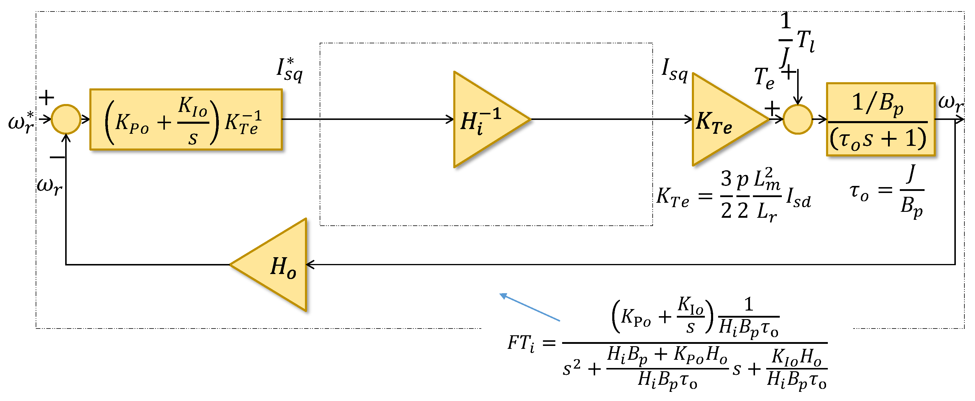
This simplified d-q model considers as an electromagnetic torque-producing current and as a rotor-flux-producing current. Then, is controlled to achieve constant rotor flux control, and is used to control the electromagnetic torque for the load demands at different rotor speeds. This way, torque and flux can be controlled independently, similar to DC machines that are separately excited, which is the aim of the IFOC (3). Figure 1 depicts the IFOC block diagram.
Remark 2.
The simplified d-q model (3) has the nonlinear terms , , and . Moreover, the load torque term is often considered as a disturbance.
The following section describes the adjustment of the basic PIC considered for rotor angular speed and stator current vector of the IFOC for IMs. This controller assumes the operation at a fixed angular rotor speed. Thus, and are constant, and model (3) behaves as an LDS. Furthermore, the outer loop PIC neglects the disturbance and expects robustness in front of its variations.
2.2. PIC Adjustment
Appendix B describes the PIC adjustment theory in detail. As a summary, the inner current controllers’ parameters are computed as follows (based on [9]):
Here, and are the direct and quadrature stator voltage references, and are the PICs inner proportional and integral parameters, and are the direct and quadrature stator current errors, is the electrical time-constant, is the inverter gain, and is the current sensor gain.
As design criteria, a root locus method is often applied. The inner damping coefficient value is chosen between and , with the most common value for this application considering . The inner natural frequency equals [51], which in this AC drive case should be higher than the switching frequency of the inverter´s IGBTs, having a value between 1.7 kHz and 16 kHz for powers between 1500 kW and 37 kW, respectively [52].
Moreover, the outer angular speed controllers’ parameters are computed as follows (based on [9]):
where is the quadrature stator current set point, and are the PICs outer proportional and integral parameters, is the rotor angular speed error, is the mechanical time-constant, and is the speed sensor gain. Here, the squared outer natural frequency is , which is used to obtain the fixed-gain parameter of the controller after considering [51,53]. The term depending on the outer natural frequency and the outer damping coefficient is , and it is used to compute the fixed-gain parameter of the controller.
Remark 3.
Please observe that PIC adjustment depends on the knowledge of the plant parameter values. Here, the resistances vary with the motor temperature, for instance. Therefore, using an adaptive controller would assure robustness regarding parameter variations.
The following section describes the CMRAC basis this manuscript considers when proposing CAPBC.
2.3. CMRAC Basis to Be Expanded for CAPBC
The CMRAC applies to scalar LDS, with relative degree 1 of the following form:
Here, the plant parameters a and b are constant and unknown, with known . The LDS´s input and output are and , respectively.
Here, the variable is the reference model output and is the identification model output. The bounded reference trajectory is . Furthermore, and are the control and identification errors. The adaptive parameters for control are , and for identification, . The designer chooses the model parameters , and , and , are the control and identification vector information. The estimated controller parameter , and the estimated plant parameter . Finally, the ideal controller parameters fulfill the following condition:
Once this CMRAC is applied to system (6) and it is assumed that , the obtained closed-loop autonomous system ensures that , , , and tend asymptotically to zero.
Figure 2 shows the CMRAC control diagram for LDS dynamical systems.
Remark 4.
The C approach enhances the D and I approaches by taking into account the closed-loop estimation error. However, it does not apply to NLDS with disturbances and unmodeled dynamics. Furthermore, CMRAC has had tuning issues for Kc and Ki, which have recently been resolved [27].
Based on the previous background and as a solution to the described issues, the following section proposes a robust CAPBC for MIMO NLDS.
3. Proposed CAPBC
This section outlines the proposed CAPBC, which combines the D and I approaches, considering the closed-loop estimation error of the adaptive parameters based on the CMRAC ideas [41,42,43] described in Section 2.3. Additionally, the proposal is adaptive and does not rely on explicit knowledge of the plant parameters, as in the case of PIC described in Section 2.2. However, this CAPBC has specific tuning formulas similar to the PIC, but depending on the known plant operational expansion the DAPBC [27], and applies to both LDS and NLDS with disturbances and unmodeled dynamics. Consequently, the proposal solves the issues described in Remark 4 of CMRAC.
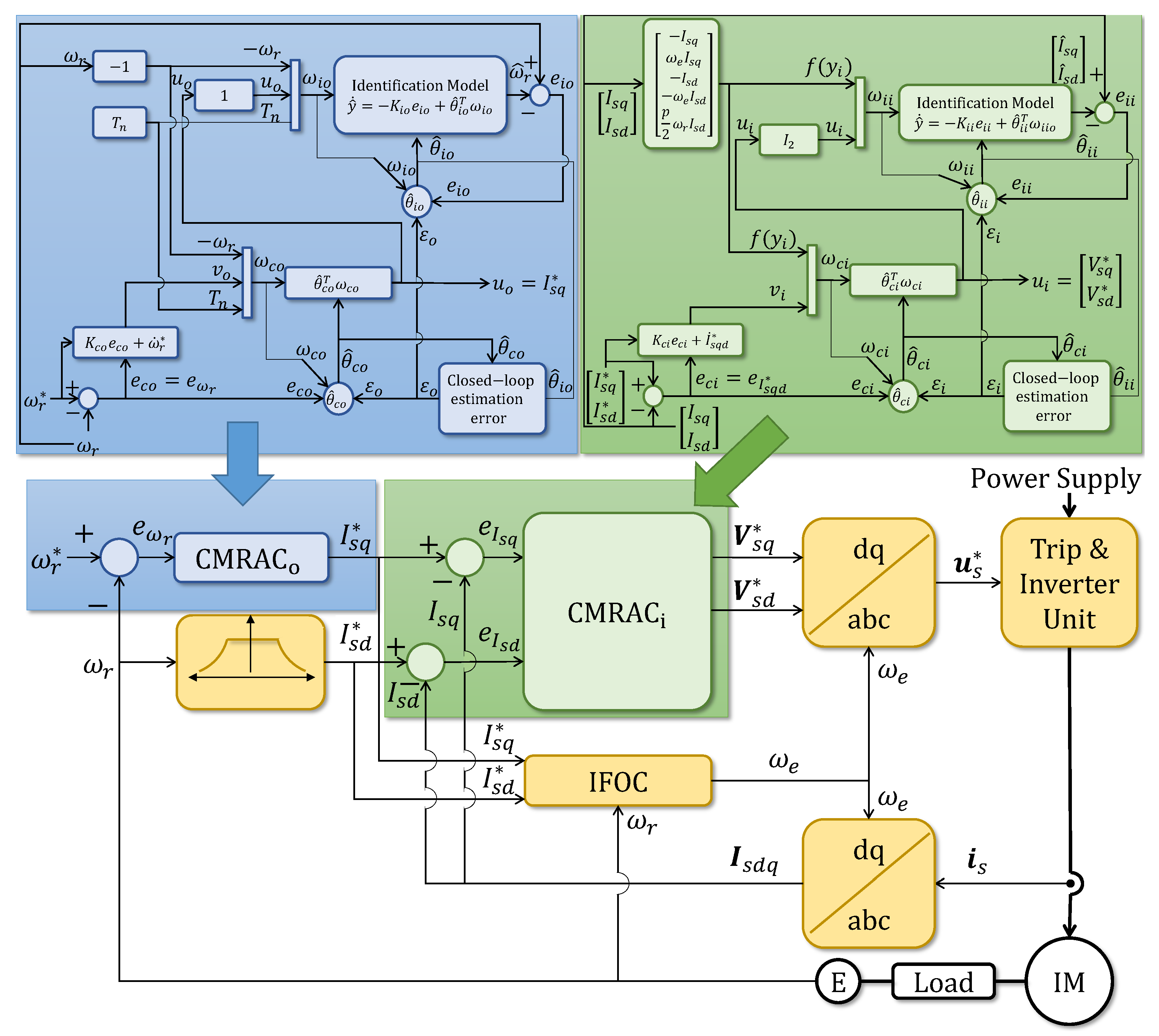
Figure 3 illustrates the proposed CAPBC diagram, which is then applied to the inner and outer control loops of the IFOC diagram described in Section 2.1 for IMs.
The proposed CAPBC shown in Figure 3 lacks of a reference model [41] and applies to MIMO dynamical systems of the following form:
Here, the output and the input are accessible. The functions , and are known, like the disturbance portion . The unmodeled dynamics are unknown, as well as the plant parameters , .
The following theorem details the proposal for the class of NLDS (14):
Theorem 1.
Here, and are the gradients of the design Lyapunov-type energy functions and . The control and identification errors are and , with . The adaptive controller and identification parameters are and , depending on the control and identification adaptive law modifications and , which are positive-definite. The information vectors for control and identification are and , where and . The auxiliary known parameters and , where and are identity matrices of order m and n, respectively. Moreover, and are null matrices of order n and m, respectively. The estimated plant parameter (19) finds , , and . The estimated controller parameter (17), computes , , and . Later, these results allow implementing the closed-loop estimation error (18).
The designer adjusts the control and identification gains , , and , where , , where and are the vectors containing the upper operational range of each element of and . Also, it adjusts the forgetting factors and [54]—(Section 4.3.6) and (Remark 4.3.7). Furthermore, the designer adjusts controller parameters and . The ideal control and identification parameters are and , which are defined as follows:
The error of the parameters are and .
Appendix C describes the CAPBC stability proof. ⋄
The proposed CAPBC is utilized in an IFOC scheme for IMs, as depicted in Figure 4.
The design considers the simplified IM d-q model (3) and divides it into the electrical and mechanical subsystems to be controlled in cascade. The first two equations of (3) represent the inner-loop electrical subsystem, with an inner output of the form and an inner control input of the form . On the other hand, the last equation of (3) represents the outer-loop mechanical subsystem, with an outer output of the form and an outer control input of the form .
The design of the outer loop controller considers the known disturbance portion to be equal to the nominal torque , and there is no disturbance for the inner loop. The function is equal to 1, and is equal to . Moreover. the design of the inner controller assumes there is no disturbance and that there are unmodelled dynamics of the inverter. The function is equal to the identity matrix of order two , and is equal to .
The design Lyapunov-type energy functions are and for the outer loop, and and for the inner loop. Therefore, their respective gradients are , , , and .
The following section discusses the obtained comparative experimental results.
4. Experimental Results
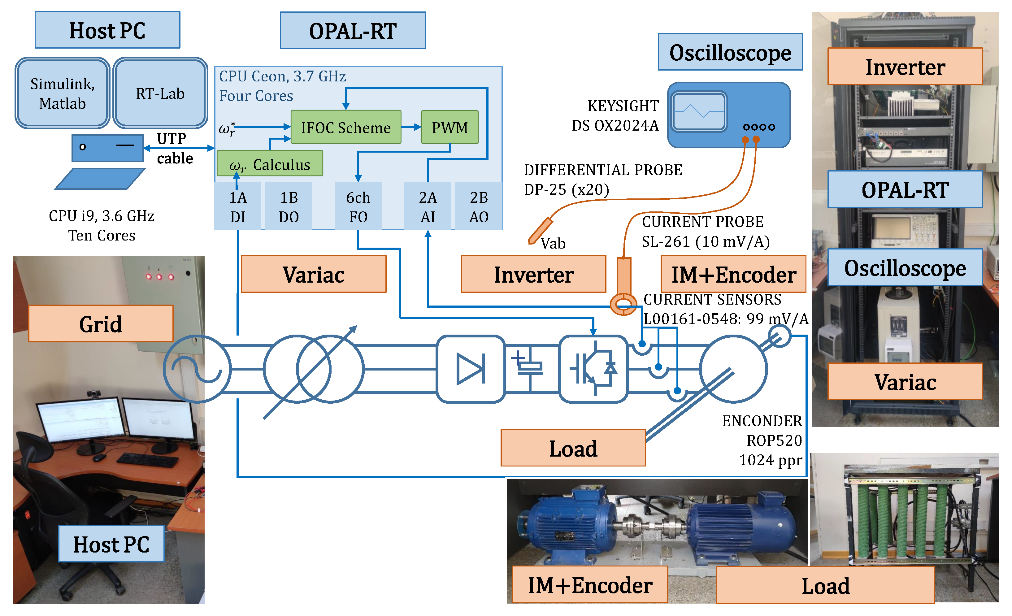
Figure 5 shows the pictures of the test bench used to validate the proposal, joined with its control diagram.
It has a real-time simulator controller OPAL-RT 4510 v2 from OPAL-RT Technologies, Montréal, QC, Canada that inherently uses a bipolar pulse width modulation (PWM), switching at 8 kHz. It commands a two-level voltage source inverter that feeds an IM-load assembly, sending the trip pulses via fiber optic (FO) cables. Simulink version 10.4 of Matlab R2021b (9.11.0.1769968) for Win64 running on a Host PC allows building the IFOC scheme of Figure 1 using PIC, DAPBC, and the proposed CAPBC and downloading them to the control platform using the software RT-LAB v2020.2.2.82. The motor data plate has 7500 kW, 380 V, 50 Hz, 1455 rpm, , and two pairs of poles . A rotor time constant of was used to implement FOC (2), which is taken from previous measurements ([16], Tables IV, Motor II).
The following controllers were programmed into the IFOC scheme:
- PIC (4) and (5). These controllers were adjusted as described in Section 2.2 and using the motor load parameter values from [16] (Tables III, IM 2) that followed the IEEE standard 112A, including DC injection, locked rotor, and free load [13] (Section 5.9).
- Proposed CAPBC from Theorem 1. It also uses both a SISO controller and a MIMO controller , as in Figure 4.
The same 10 s duration test applies to the PIC, DAPBC, and proposed CAPBC strategies. It considers that the IM starts with a torque load and applies a step speed command of 25 rad/s, 60 rad/s, 85 rad/s, 120, and rad/s, at times 2 s, s, 3 s, s, and 4 s, respectively. Later, the load decreases to at 5 s and increases again to at 6 s. Finally, the field disorientation is considered by adjusting the value of from IFOC (2) to at s and increases again to at 9 s, simulating step changes for the rotor time constant.
Figure 6 exhibits the controller’s comparative rotor angular speed response. It can be seen that adaptive controllers are more robust against different variations, including load torque and IFOC-impacting parameter variations. All controllers track the reference speed. However, adaptive controllers exhibit lower maximum overshoot (MO) and faster response than PIC in all scenarios. Here, the proposed CAPBC has the lowest MO and the fastest response. The effectiveness of the proposed CAPBC is superior for the different step changes in the reference speed occurring every s until 4 s, as well as for the torque and IFOC variations. The CAPBC enhanced the transient response of the PIC and the DAPBC, as expected.
The CMRAC exhibits the best performance in all scenarios despite having similar steady-state errors () across the different controllers. The proposal demonstrates the lowest control effort (please see the ISI index) and better transient behavior with the lowest MO and IAE indexes. The performance of the PIC deteriorates significantly when field disorientation occurs at seven and nine seconds with equal to and , respectively. The proposed CAPBC and DAPBC for the inner loop ensure robustness under this situation due to their MIMO, adaptive natures, and NLDS designs.
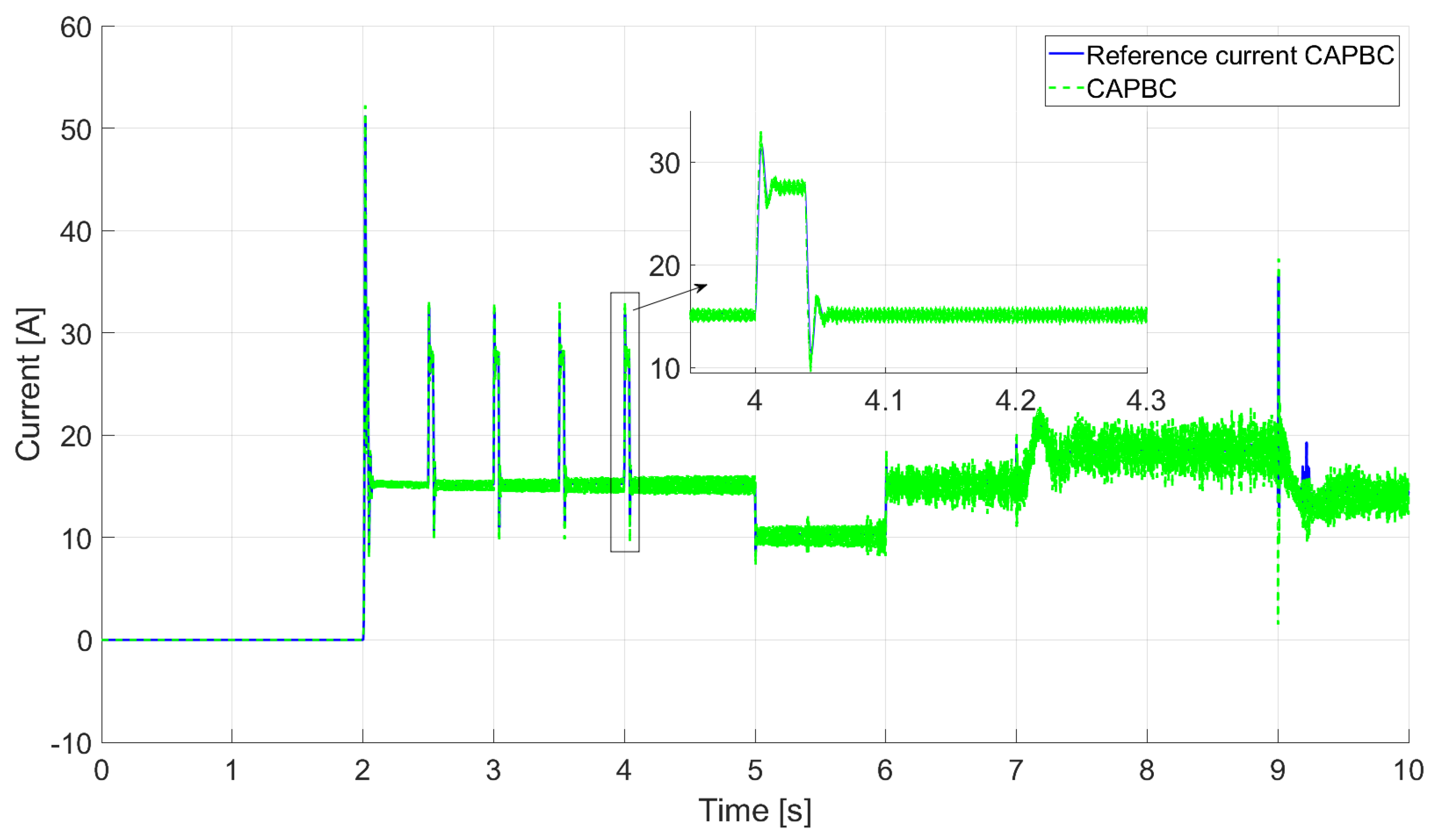
Figure 7, Figure 8 and Figure 9 show the consumed and reference q-axis current for torque production for the PIC, DPABC, and CAPBC, respectively. All controllers track the reference current that produces torque, with CMRAC and DAPBC having a faster response than PIC. The PIC has difficulties tracking the reference after nine seconds when field disorientation occurs, as seen in the center-right side of Figure 7. This provokes the tracking difficulties shown in the upper-right side of Figure 6 for the slower speed control outer loop.
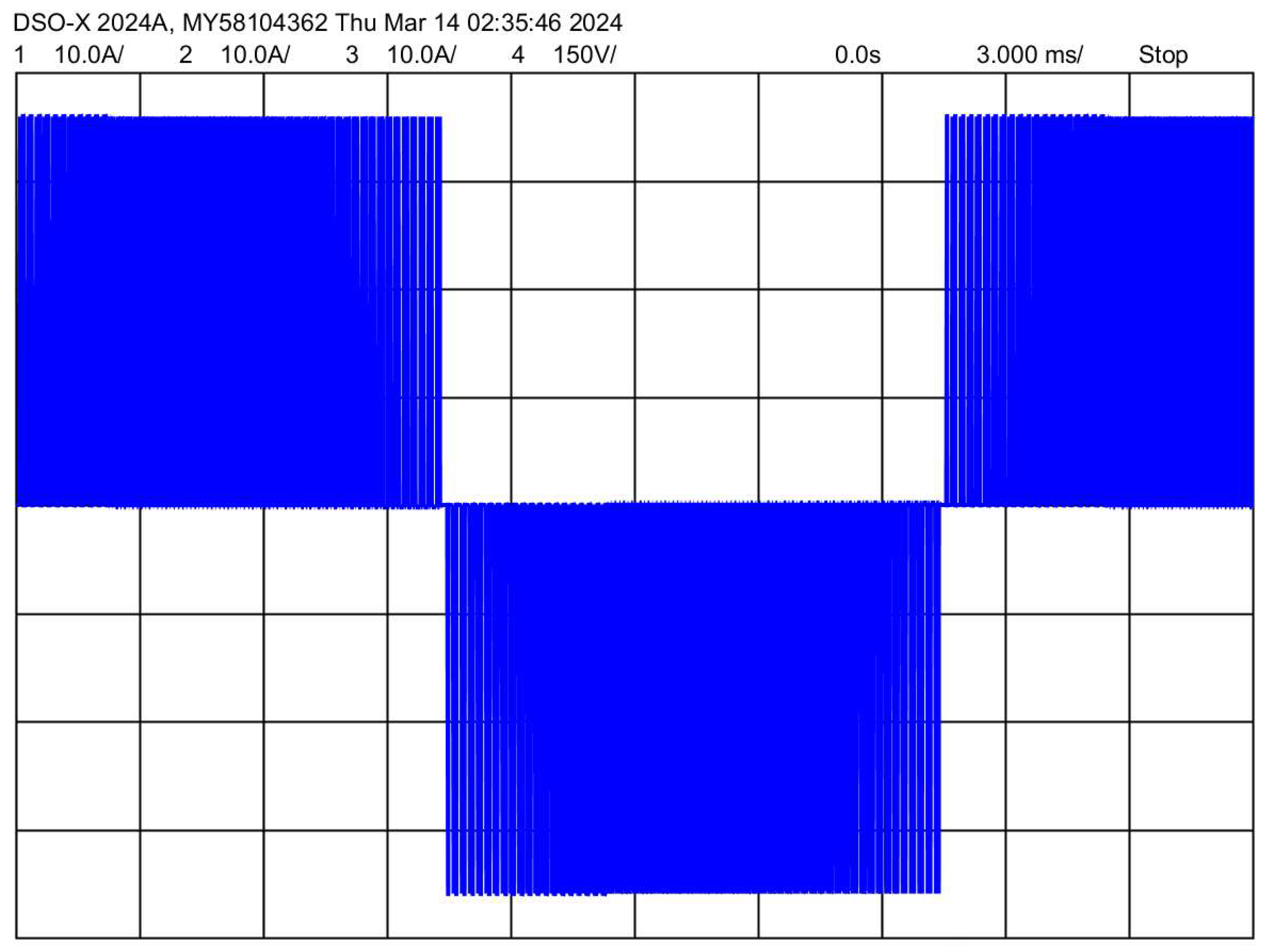
It can be seen in Figure 7, Figure 8 and Figure 9 that the faster speed responses of adaptive controllers are achieved with a higher reference and consumed q-axis current torque producing, as expected. Moreover, the line voltages have the typical PWM wayform, with the 50 Hz frequency corresponding to the nominal rotor angular speed, as can be seen in Figure 10, Figure 11 and Figure 12.
5. Conclusions
This paper introduced a novel CAPBC tailored for a class of nonlinear systems encompassing the IMs under an IFOC scheme, including perturbances and unmodeled dynamics. It expands the DAPBC technique [27] based on the combined approach previously proposed for MRAC [41,42,43]. The theoretical underpinnings of the proposed CAPBC are detailed in Theorem 1, and the stability proof is exhibited in Appendix C.
Later, the proposal implemented a SISO CAPBC angular speed control for the outer loop of an IFOC for IMs in cascade with the inner-loop MIMO CAPBC d-q axis current control. This paper presents comparative experimental results between the proposed CAPBC, the DAPBC, and PIC techniques in an IFOC scheme for an IM of 7.5 kW. The results demonstrate that the proposed technique is effective and outperforms DAPBC and PIC techniques. Unlike traditional PICs, the CAPBC does not need knowledge of the motor load parameters.
Author Contributions
Conceptualization, methodology, writing—original draft preparation, and visualization, J.C.T.-T.; investigation, formal analysis, supervision, project administration, data curation, and resources and funding acquisition, J.C.T.-T., A.J.R.-M. and N.A.-C.; validation, software, and writing—review and editing; A.J.R.-M. and N.A.-C. All authors have read and agreed to the published version of the manuscript.
Funding
This research was funded by ANID Chile, grant IT23I0117; FONDECYT Chile, grant 1220168; This work was funded by the National Agency for Research and Development (ANID)/Scholarship Program/DOCTORADO BECAS CHILE/2023-21230599.
Data Availability Statement
Data are contained within the article.
Conflicts of Interest
The authors declare no conflicts of interest.
Abbreviations
The following abbreviations are used in this manuscript:
| IMs | Induction motors |
| DC | Direct current |
| AC | Alternating current |
| D | Direct approach |
| I | Indirect approach |
| C | Combined approach |
| VSDs | Variable speed drives |
| FOC | Field-oriented control |
| VSDs | Variable speed drives |
| DTC | Direct torque control |
| IFOC | Indirect field-oriented control |
| LDS | Linear dynamical systems |
| NLDS | Nonlinear dynamical systems |
| PIC | Proportional and integral controller |
| MRAC | Model reference adaptive control |
| DMRAC | Direct model reference adaptive control |
| CMRAC | Combined model reference adaptive control |
| APBC | Adaptive passivity-based control |
| DAPBC | Direct adaptive passivity-based control |
| SMC | Sliding mode control |
| ANN | Artificial neural network |
| PSO | Particle swarm optimization technique |
| SISO | Single-input and single-output |
| MIMO | Multiple-input and multiple-output |
| KCD | Known control direction |
| PWM | Pulse width modulation |
| Ess [%] | Steady-state error computed as at the response ending |
| MO [%] | Maximum overshoot calculated as at the response starting |
| IAE [cm.s] | Integral absolute value Error of the output |
| ISI [] | Integral squared output |
| Mathematical Operators | |
| Continuous first-time derivative of x. | |
| Estimated variable or parameter x. | |
| Set-point or required output variable y. | |
| e,m | Referred to electrical e and mechanical m. |
| i,o | Inner and outer variable. |
| Transpose vector variable y. | |
| , and | Functions of the variable y. |
| Main Notation | |
| The following main notations are used in this manuscript: | |
| , | Rotor and electrical angular speed |
| Rotor position | |
| Stator voltage | |
| Stator current | |
| , , and | Electromagnetic, load, and nominal torque. |
| p | Number of poles |
| and | Stator and rotor resistance |
| and | Stator and rotor leakage inductance |
| , , and | Stator, rotor, and magnetizing inductance |
| Leakage or coupling coefficient, given by | |
| Stator transient resistance, with | |
| Stator transient time constant. Given by | |
| Rotor time constant | |
| , and | Electrical and mechanical time constant |
| Mechanical friction factor | |
| J | Moment of inertia |
| , and | Direct and quadrature stator current amplitudes |
| , and | Direct and quadrature stator voltage amplitudes |
| , and | Direct and quadrature stator current errors |
| Rotor angular speed error | |
| , and | Direct and quadrature rotor flux amplitudes |
| Constant | |
| and | PICs proportional and integral parameters |
| , and | Inverter and speed sensor gain |
| Damping coefficient | |
| Natural frequency | |
| y, and | Plant and reference model output |
| a, b, A, B, and | Plant parameters |
| , , , , and | Model parameters |
| , and | Control and identification errors |
| , and | Adaptive parameters for control and for identification |
| , and | Control and identification vector information |
| , and | Vectors containing the upper operational range of each element of and |
| Closed-loop estimation error | |
| Disturbance portion | |
| Unmodeled dynamics | |
| , and | Gradients of the design Lyapunov-type energy functions |
| , and | Positive-definite constants |
| , and | Auxiliary known parameters |
| , and | Identity matrix of order m and n |
| , and | Null matrix of order m and n |
| , and | Control, identification, and closed-loop estimation error gains |
| , and | Forgetting factors |
Appendix A. IFOC Method Basis
The basic IFOC method [55] imposes an electrical angular frequency equal to
Here, substituting (A1) into the first derivatives of the direct and quadrature rotor flux and of Equation (1), these rotor fluxes dynamical equations from (1) take the form
Then, if the term in this last equation with accurate estimations, the dynamical equation of the quadrature rotor flux component has an exponential behavior tending to zero over time , reaching over the 99% of this final value after five times the rotor-time constant [9]. Later, and the electromagnetic torque , obtaining the simplified model (3).
However, using Equation (A1) to achieve IFOC needs a flux estimator to obtain , which is the reason why it is not used in this paper. Therefore, the alternative and more practical method using the electrical angular frequency of Equation (2) is performed in this paper [49,56].
The authors have not found explicit proof of this method in the literature. Thus, we describe it herein. After considering the definition of the rotor time constant and substituting Equation (2) into the third and fourth equations of (1), the rotor flux dynamical equations from (1) take the form
After applying the Laplace transform [56] to this last equation, considering constant and the initial condition , we obtain
Applying the final value theorem [56], where , we have . As a result, . Then, . Here, if , we obtain , achieving field orientation. This could be obtained under the presence of accurate parameters estimation, similar to the basic IFOC method, thus ; and even if and , but , which is a valid case not considered in [56].
Appendix B. PIC Adjustment
The adjustment of the PI controllers starts from the simplified IM d-q model (3) and the IFOC block diagram of Figure 1. These are re-expressed as the transfer function block diagram [53] of Figure A1 in Laplace domain after considering all the motor load parameters and the operating point constant is known.
The inner loop is first adjusted after neglecting the nonlinear terms and . Moreover, it considers the closed-loop transfer functions property of with and [53], obtaining the transfer function shown in Figure A1, of the form . Here, the squared inner natural frequency is used to obtain the fixed-gain parameter of the controller. The term depending on the inner natural frequency and the inner damping coefficient is ; and it is used to compute the fixed-gain parameter of the controller. The inner PICs adjustment results in Equation (4).
Later, it is assumed that the inner loop is stabilized. Therefore, applying the final value theorem [56], where , we have that and the block diagram of Figure A1 is achieved.
In a similar way to the inner loop, after considering the load torque term as a disturbance that is neglected, and considering the closed-loop transfer functions property, the transfer function is obtained [51,53]. Here, the squared outer natural frequency is , and it is used to obtain the fixed-gain parameter of the controller. The term , depending on the outer natural frequency and the outer damping coefficient, is used to compute the fixed-gain parameter of the controller. Finally, the outer PIC is adjusted as in Equation (5).
Figure A1.
Transfer function block diagram of Basic IFOC for IM.
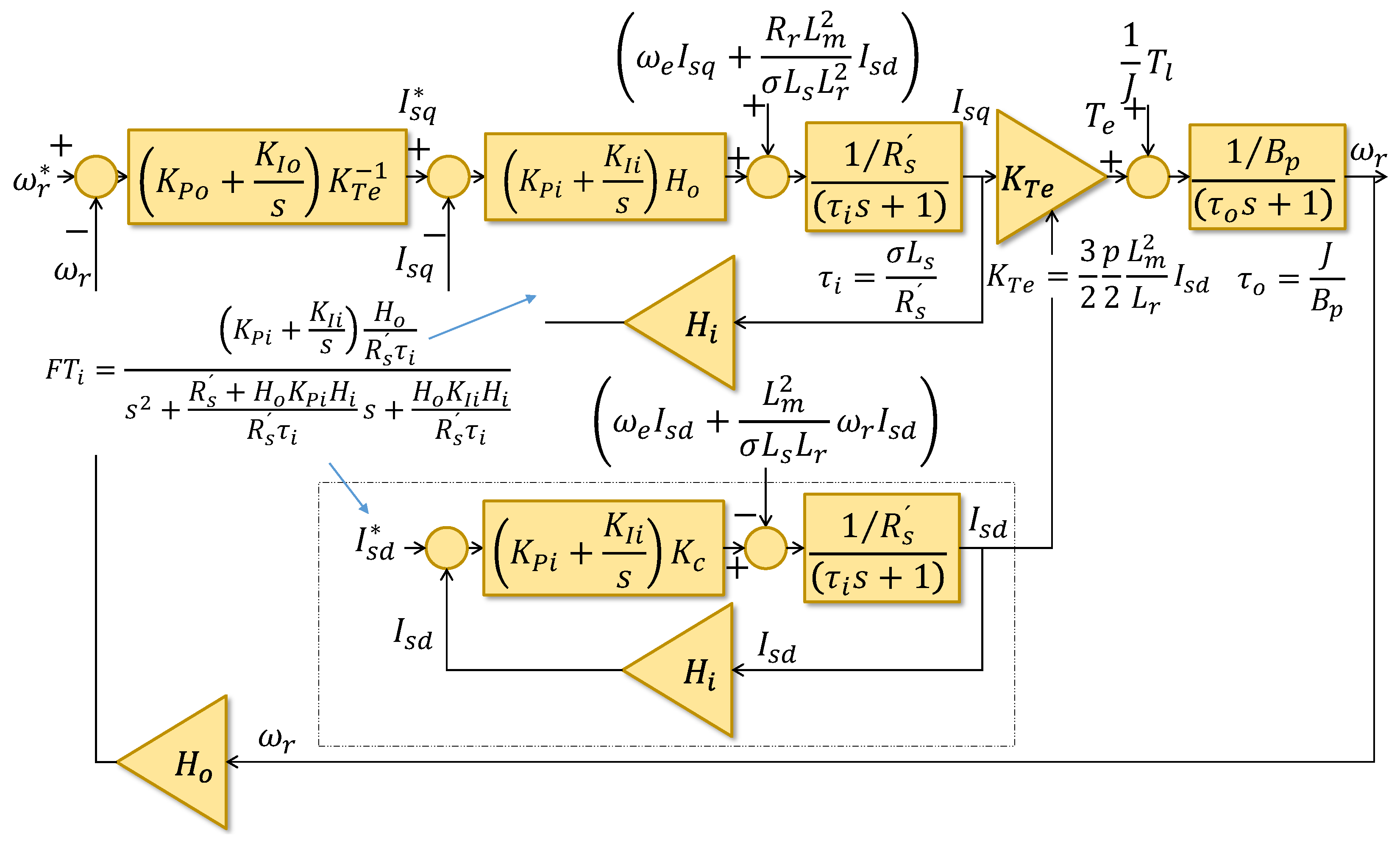
Figure A2.
Transfer function block diagram of basic IFOC for IM once the inner loop is stabilized.
Appendix C. CAPBC Stability Proof
Obtaining the Error Dynamical Equations
Subtracting Equations (14) from (15) and regrouping terms, the following identification error is obtained:
It considers the previously given definitions of , , . Moreover, the identification parameter error is defined as .
Multiplying both sides of the model plant (14) by , adding and subtracting the term , regrouping and considering previous definitions of , , , the control error is
where .
In contrast to D and I approaches, the C technique considers , and , obtaining the closed-loop estimation error (18).
Subtracting (18) from (21) (since (21) being equal to zero does not change the equation), to the right side, respectively, and regrouping terms, we obtain
.
This result equals
Finally, as and , and the identification and control ideal parameters and are constant, we have that and . Therefore, from (17) and (19), we have
Stability Proof of the Error Dynamical Equations
The system composed by the errors dynamical Equations (A5), (A6), (A8) and (A9) has an associated Lyapunov function, which is positive and depends on the design energy function .
The first time derivative of (A10) gives
Regrouping terms, it gives:
Now, considering , and , and regrouping terms, it follows that
Moreover, the authors consider the two vectors’ properties, where , to write the terms and into the trace as follows:
Simplifying the last equation, after canceling identical terms with opposite signs and regrouping the terms with conveniently to obtain Equation (A7), gives
In this scenario, we assume that all parameters involved, , , , , , and , are strictly positive. Additionally, we know that the parameters characterizing the plant, along with their first derivatives with respect to time, remain within certain bounds.
However, upon inspection of Equation (A12), it becomes evident that while the first terms indicate negativity, the signs of the subsequent four terms are not immediately discernible. To address this ambiguity, we aim to reformulate Equation (A12) using modulus and norm properties, as demonstrated in [38].
Using properties of the Frobenius norm and the Cauchy–Schwarz inequality where , the terms become , , and . Using the property , we have , , and .
Therefore, only outside the region , which is the following instability hyperelliptic paraboloid that is compact, closed, and includes the following origin:
Hence, using Lyapunov’s second method, it can be concluded that the variables of the closed-loop dynamical Equations (A5), (A6), (A8) and (A9) are bounded outside . In case the errors take small enough values that result in (inside the instability compact and closed region , including the origin); these will be pushed back to a stable boundary. In practice, the values of , , , , and are chosen so that the permanent errors are as a small as possible, as can be seen in the following section.
Thus, , , , and are bounded outside , i.e., , , , and outside . Since and are bounded, it implies that y, and are bounded as is a bounded reference. As and are bounded, and we have bounded plant parameters, then the adaptive parameters and are bounded, since and . Having all these bounded signals outside , and that V, , , and , from (A5), (A6), (A8) and (A9), we have that , , and .
Integrating both sides of in the interval gives
as V is bounded outside , from the right-hand side of this last equation, we have and outside .
Furthermore, as , and , and , and , all outside , using Barbalat´s Lemma [30] (Section 4.5.2) we have that and , both tend asymptotically to zero outside . Hence, and outside . We do not ensure parameter convergence. This concludes the proof. ⋄
References
- Ivanov-Smolenskij, A.; Kuznecov, B. Electrical Machines: Vol. 1; Mir: Moscow, Russia, 1983. [Google Scholar]
- Hannan, M.; Ali, J.A.; Mohamed, A.; Hussain, A. Optimization techniques to enhance the performance of induction motor drives: A review. Renew. Sustain. Energy Rev. 2018, 81, 1611–1626. [Google Scholar] [CrossRef]
- Travieso-Torres, J.C.; Contreras-Jara, C.; Diaz, M.; Aguila-Camacho, N.; Duarte-Mermoud, M.A. New Adaptive Starting Scalar Control Scheme for Induction Motor Variable Speed Drives. IEEE Trans. Energy Convers. 2021, 37, 729–736. [Google Scholar] [CrossRef]
- Depenbrock, M. Direkte selbstregelung (DSR) für hochdynamische drehfeldantriebe mit stromrichterspeisung. etz-Archiv 1985, 7, 211–218. [Google Scholar]
- Vas, P. Sensorless Vector and Direct Torque Control. Oxf. Univ. Press Google Sch. 1998, 2, 265–273. [Google Scholar]
- Hasse, K. Zur Dynamic Drehzahlgeregelter Antriebe mit Stromaschinen. Ph.D. Thesis, Technische Hochschule Darmstadt, Darmstadt, Germany, 1969. [Google Scholar]
- Blaschke, F. The principle of field orientation as applied to the new transvector closed-loop control system for rotating-field machine. Siemens Rev. 1772, 34, 217–220. [Google Scholar]
- Desoer, C.; Lin, C.A. Tracking and disturbance rejection of MIMO nonlinear systems with PI controller. IEEE Trans. Autom. Control 1985, 30, 861–867. [Google Scholar] [CrossRef]
- Ogata, K. Ingeniería de Control Moderna; Pearson Educación: London, UK, 2003. [Google Scholar]
- Sengamalai, U.; Anbazhagan, G.; Thamizh Thentral, T.; Vishnuram, P.; Khurshaid, T.; Kamel, S. Three phase induction motor drive: A systematic review on dynamic modeling, parameter estimation, and control schemes. Energies 2022, 15, 8260. [Google Scholar] [CrossRef]
- Amaral, G.F.V.; Baccarini, J.M.R.; Coelho, F.C.R.; Rabelo, L.M. A high precision method for induction machine parameters estimation from manufacturer data. IEEE Trans. Energy Convers. 2020, 36, 1226–1233. [Google Scholar] [CrossRef]
- Perin, M.; Pereira, L.A.; Silveira, G.B.; Haffner, S. Estimation of the parameters for multi-cage models of induction motors using manufacturer data and PSO. In Electrical Engineering; Springer: Berlin/Heidelberg, Germany, 2023; pp. 1–19. [Google Scholar]
- Engineers, E.; Board, I. 112-2017—IEEE Standard Test Procedure for Polyphase Induction Motors and Generators; IEEE: Piscataway, NJ, USA, 2018; pp. 1–115. [Google Scholar] [CrossRef]
- Yoo, J.; Lee, J.H.; Sul, S.K. FEA-Assisted Experimental Parameter Map Identification of Induction Motor for Wide-Range Field-Oriented Control. IEEE Trans. Power Electron. 2023, 39, 1353–1363. [Google Scholar] [CrossRef]
- Véliz-Tejo, A.; Travieso-Torres, J.C.; Peters, A.A.; Mora, A.; Leiva-Silva, F. Normalized-Model Reference System for Parameter Estimation of Induction Motors. Energies 2022, 15, 4542. [Google Scholar] [CrossRef]
- Travieso-Torres, J.C.; Lee, S.S.; Veliz-Tejo, A.; Leiva-Silva, F.; Ricaldi-Morales, A. Self-Commissioning Parameter Estimation Algorithm for Loaded Induction Motors. IEEE Trans. Ind. Electron. 2024, 1–11. [Google Scholar] [CrossRef]
- Travieso-Torres, J.C.; Duarte-Mermoud, M.A. Two simple and novel SISO controllers for induction motors based on adaptive passivity. ISA Trans. 2008, 47, 60–79. [Google Scholar] [CrossRef] [PubMed]
- Talla, J.; Leu, V.Q.; Šmídl, V.; Peroutka, Z. Adaptive speed control of induction motor drive with inaccurate model. IEEE Trans. Ind. Electron. 2018, 65, 8532–8542. [Google Scholar] [CrossRef]
- Kilic, E.; Ozcalik, H.R.; Yilmaz, S. Efficient speed control of induction motor using RBF based model reference adaptive control method. Autom. Časopis Za Autom. Mjer. Elektron. Računarstvo I Komun. 2016, 57, 714–723. [Google Scholar] [CrossRef]
- Zellouma, D.; Bekakra, Y.; Benbouhenni, H. Field-oriented control based on parallel proportional–integral controllers of induction motor drive. Energy Rep. 2023, 9, 4846–4860. [Google Scholar] [CrossRef]
- Sudheer, A.; Aware, M.V. Improved fractional order speed controller with non-linear vsi-im model to enhance the load disturbance capability. ISA Trans. 2023, 142, 538–549. [Google Scholar] [CrossRef] [PubMed]
- Aziz, A.G.M.A.; Abdelaziz, A.Y.; Ali, Z.M.; Diab, A.A.Z. A comprehensive examination of vector-controlled induction motor drive techniques. Energies 2023, 16, 2854. [Google Scholar] [CrossRef]
- Adigintla, S.; Aware, M.V. Robust fractional order speed controllers for induction motor under parameter variations and low speed operating regions. IEEE Trans. Circuits Syst. II Express Briefs 2022, 70, 1119–1123. [Google Scholar] [CrossRef]
- Zellouma, D.; Bekakra, Y.; Benbouhenni, H. Robust synergetic-sliding mode-based-backstepping control of induction motor with MRAS technique. Energy Rep. 2023, 10, 3665–3680. [Google Scholar] [CrossRef]
- Ali, S.; Prado, A.; Pervaiz, M. Hybrid backstepping-super twisting algorithm for robust speed control of a three-phase induction motor. Electronics 2023, 12, 681. [Google Scholar] [CrossRef]
- Yang, G.; Yao, J. Multilayer neurocontrol of high-order uncertain nonlinear systems with active disturbance rejection. Int. J. Robust Nonlinear Control 2024, 34, 2972–2987. [Google Scholar] [CrossRef]
- Travieso-Torres, J.C.; Duarte-Mermoud, M.A.; Díaz, M.; Contreras-Jara, C.; Hernández, F. Closed-Loop Adaptive High-Starting Torque Scalar Control Scheme for induction Motor Variable Speed Drives. Energies 2022, 15, 3489. [Google Scholar] [CrossRef]
- Ioannou, P.A.; Sun, J. Robust Adaptive Control; PTR Prentice-Hall: Upper Saddle River, NJ, USA, 1996; Volume 1. [Google Scholar]
- Åström, K.J.; Wittenmark, B. Adaptive Control; Courier Corporation: North Chelmsford, MA, USA, 2008. [Google Scholar]
- Narendra, K.; Annaswamy, A. Stable Adaptive Systems; Dover Books on Electrical Engineering; Dover Publications: Mineola, NY, USA, 2012. [Google Scholar]
- Tiwari, M.; Prazenica, R.; Henderson, T. Direct adaptive control of spacecraft near asteroids. Acta Astronaut. 2023, 202, 197–213. [Google Scholar] [CrossRef]
- Artuc, M.B.; Bayezit, I. Robust adaptive quadrotor position tracking control for uncertain and fault conditions. Proc. Inst. Mech. Eng. Part G J. Aerosp. Eng. 2023, 237, 3172–3184. [Google Scholar] [CrossRef]
- Wang, Y.; Shen, C.; Huang, J.; Chen, H. Model-free adaptive control for unmanned surface vessels: A literature review. Syst. Sci. Control Eng. 2024, 12, 2316170. [Google Scholar] [CrossRef]
- Liu, Z.; Zhao, Y.; Zhang, O.; Chen, W.; Wang, J.; Gao, Y.; Liu, J. A Novel Faster Fixed-Time Adaptive Control for Robotic Systems With Input Saturation. IEEE Trans. Ind. Electron. 2023, 71, 5215–5223. [Google Scholar] [CrossRef]
- Burghi, T.; Iossaqui, J.; Camino, J. A general update rule for Lyapunov-based adaptive control of mobile robots with wheel slip. Int. J. Adapt. Control Signal Process. 2024, 38, 1172–1198. [Google Scholar] [CrossRef]
- Mirzaee, M.; Kazemi, R. Direct adaptive fractional-order non-singular terminal sliding mode control strategy using extreme learning machine for position control of 5-DOF upper-limb exoskeleton robot systems. Trans. Inst. Meas. Control 2024, 01423312231225605. [Google Scholar] [CrossRef]
- Abubakr, H.; Vasquez, J.C.; Mohamed, T.H.; Guerrero, J.M. The concept of direct adaptive control for improving voltage and frequency regulation loops in several power system applications. Int. J. Electr. Power Energy Syst. 2022, 140, 108068. [Google Scholar] [CrossRef]
- Travieso-Torres, J.C.; Ricaldi-Morales, A.; Véliz-Tejo, A.; Leiva-Silva, F. Robust Cascade MRAC for a Hybrid Grid-Connected Renewable Energy System. Processes 2023, 11, 1774. [Google Scholar] [CrossRef]
- Karami-Mollaee, A.; Barambones, O. Higher Order Sliding Mode Control of MIMO Induction Motors: A New Adaptive Approach. Mathematics 2023, 11, 4558. [Google Scholar] [CrossRef]
- Çavuş, B.; Aktaş, M. A New Adaptive Terminal Sliding Mode Speed Control in Flux Weakening Region for DTC Controlled Induction Motor Drive. IEEE Trans. Power Electron. 2023, 39, 449–458. [Google Scholar] [CrossRef]
- Duarte, M.A.; Narendra, K.S. Combined direct and indirect approach to adaptive control. IEEE Trans. Autom. Control 1989, 34, 1071–1075. [Google Scholar] [CrossRef]
- Duarte-Mermoud, M.A.; Rojo, F.A.; Pérez, R. Experimental evaluation of combined model reference adaptive controller in a pH regulation process. Int. J. Adapt. Control Signal Process. 2002, 16, 85–106. [Google Scholar] [CrossRef]
- Duarte-Mermoud, M.A.; Rioseco, J.S.; González, R.I. Control of longitudinal movement of a plane using combined model reference adaptive control. Aircr. Eng. Aerosp. Technol. 2005, 77, 199–213. [Google Scholar] [CrossRef]
- Lavretsky, E. Combined/composite model reference adaptive control. IEEE Trans. Autom. Control 2009, 54, 2692–2697. [Google Scholar] [CrossRef]
- Xie, J.; Yan, H.; Li, S.; Yang, D. Almost output regulation model reference adaptive control for switched systems: Combined adaptive strategy. Int. J. Syst. Sci. 2020, 51, 556–569. [Google Scholar] [CrossRef]
- Roy, S.B.; Bhasin, S.; Kar, I.N. Combined MRAC for unknown MIMO LTI systems with parameter convergence. IEEE Trans. Autom. Control 2017, 63, 283–290. [Google Scholar] [CrossRef]
- Makavita, C.D.; Nguyen, H.D.; Ranmuthugala, D.; Jayasinghe, S.G. Composite model reference adaptive control for an unmanned underwater vehicle. Underw. Technol. 2015, 33, 81–93. [Google Scholar] [CrossRef]
- Abdul Ghaffar, A.F.; Richardson, T.; Greatwood, C. A combined model reference adaptive control law for multirotor UAVs. IET Control Theory Appl. 2021, 15, 1474–1487. [Google Scholar] [CrossRef]
- Vas, P. Electrical Machines and Drives: A Space-Vector Theory Approach; Clarendon Press Oxford: Oxford, UK, 1992; Volume 1. [Google Scholar]
- Park, R.H. Two-reaction theory of synchronous machines generalized method of analysis-part I. Trans. Am. Inst. Electr. Eng. 1929, 48, 716–727. [Google Scholar] [CrossRef]
- Dorf, R.C.; Bishop, R.H. Modern Control Systems; Pearson Education, Inc.: Upper Saddle River, NJ, USA, 2011. [Google Scholar]
- Siemens. Vector Control Simovert Masterdrives VC, Single-Motor and Multi-Motor Drives 0.55 kW to 2300 kW, Catalog DA 65.10 • 2003/2004; Siemens AG: Berlin/Heidelberg, Germany, 2003. [Google Scholar]
- Schiff, J.L. The Laplace Transform: Theory and Applications; Springer Science & Business Media: Berlin/Heidelberg, Germany, 1999. [Google Scholar]
- Travieso-Torres, J.C.; Contreras, C.; Hernández, F.; Duarte-Mermoud, M.A.; Aguila-Camacho, N.; Orchard, M.E. Adaptive passivity-based control extended for unknown control direction. ISA Trans. 2022, 122, 398–408. [Google Scholar] [CrossRef] [PubMed]
- Feraga, C.E.; Sedraoui, M.; Bachir Bouiadjra, R. Enhanced Indirect Field-Oriented Control of Single-Phase Induction Motor Drive Using H∞ Current Controller. Arab. J. Sci. Eng. 2019, 44, 7187–7202. [Google Scholar] [CrossRef]
- Cao, P.; Zhang, X.; Yang, S. A unified-model-based analysis of MRAS for online rotor time constant estimation in an induction motor drive. IEEE Trans. Ind. Electron. 2017, 64, 4361–4371. [Google Scholar] [CrossRef]
Figure 1.
IFOC diagram for IMs based on [5] (Section 4.1).
Figure 1.
IFOC diagram for IMs based on [5] (Section 4.1).
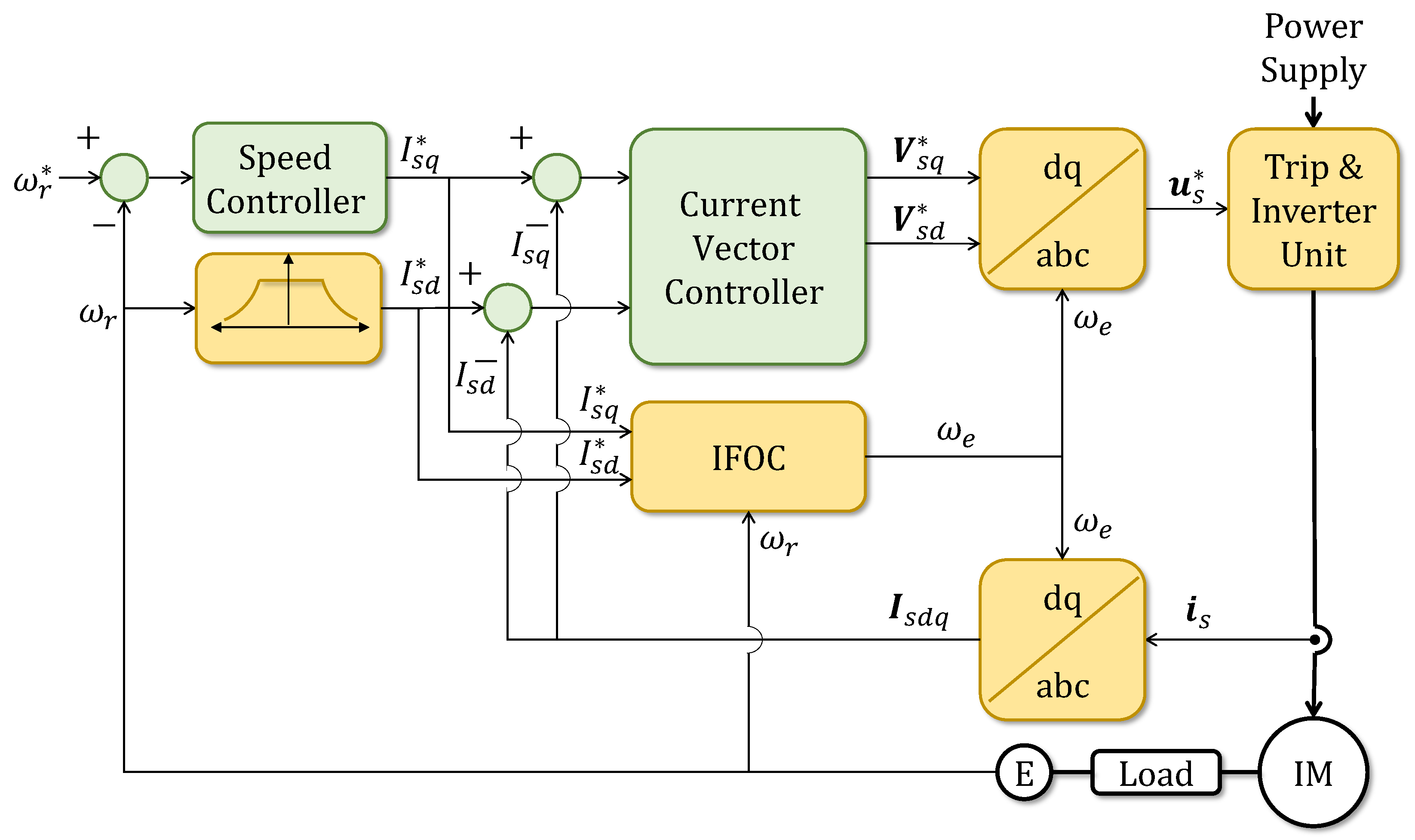
Figure 2.
CMRAC diagram based on [41].
Figure 2.
CMRAC diagram based on [41].
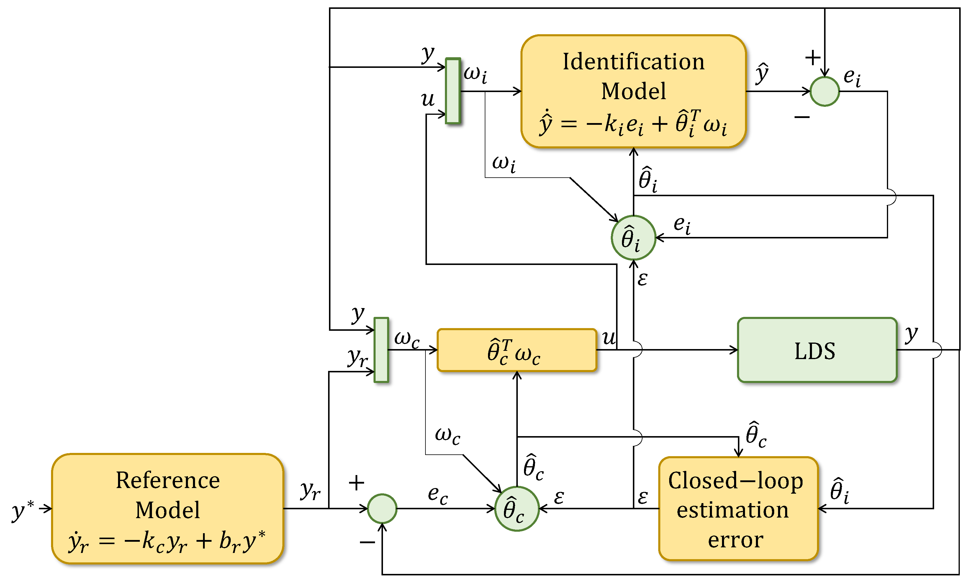
Figure 3.
Proposed CAPBC diagram for MIMO NLDS; the differences are marked in red.
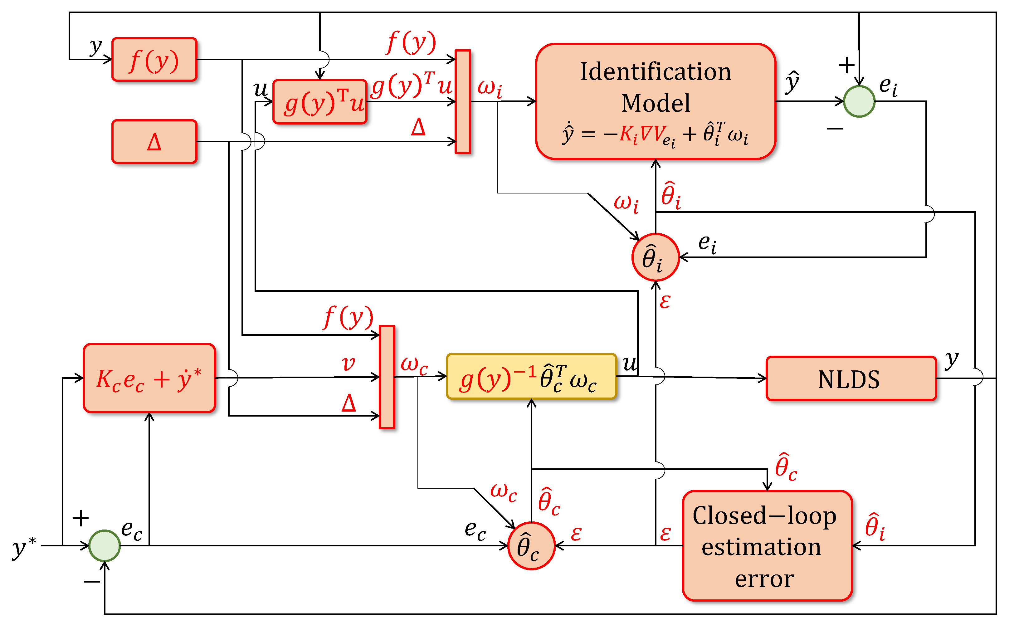
Figure 4.
IFOC diagram for IMs with the proposed CAPBCs.

Figure 5.
Test bench pictures and control diagram.

Figure 6.
Comparative rotor angular speed.

Figure 7.
Consumed and reference q-axis current torque producing for PIC.
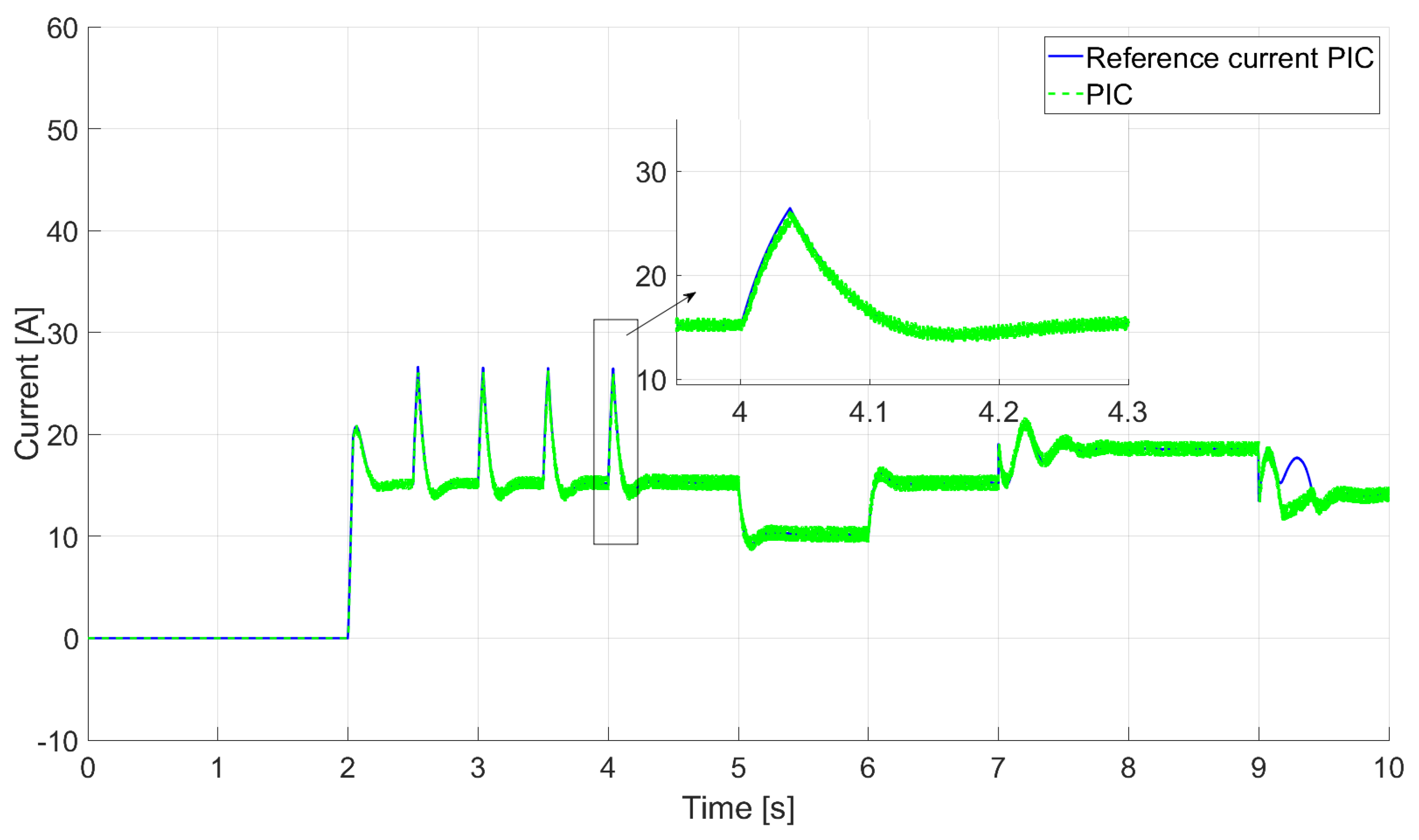
Figure 8.
Consumed and reference q-axis current torque producing for DAPBC.
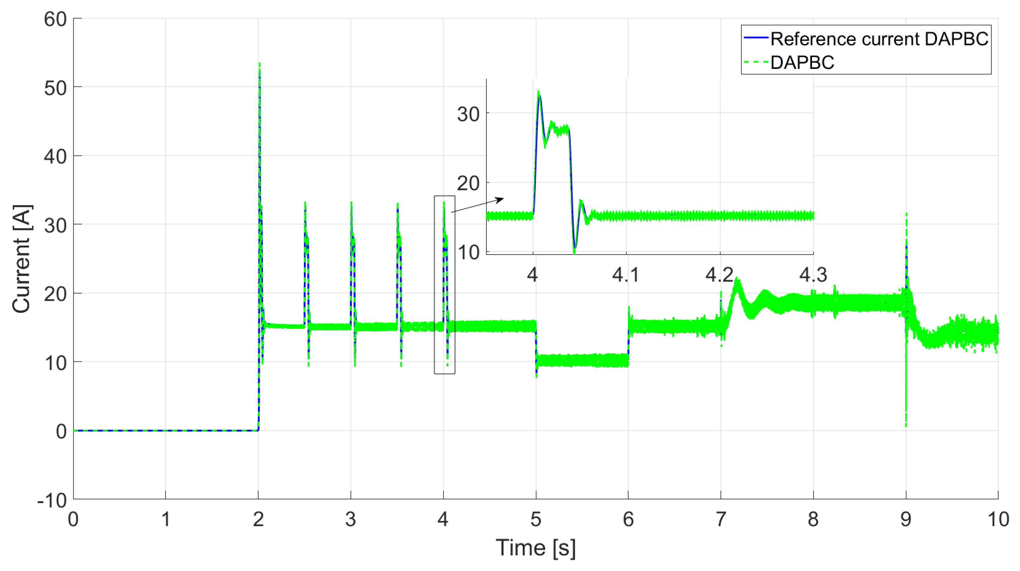
Figure 9.
Consumed and reference q-axis current torque producing for the proposed CAPBC.

Figure 10.
Line voltage a-b around second 6.5 for PIC.

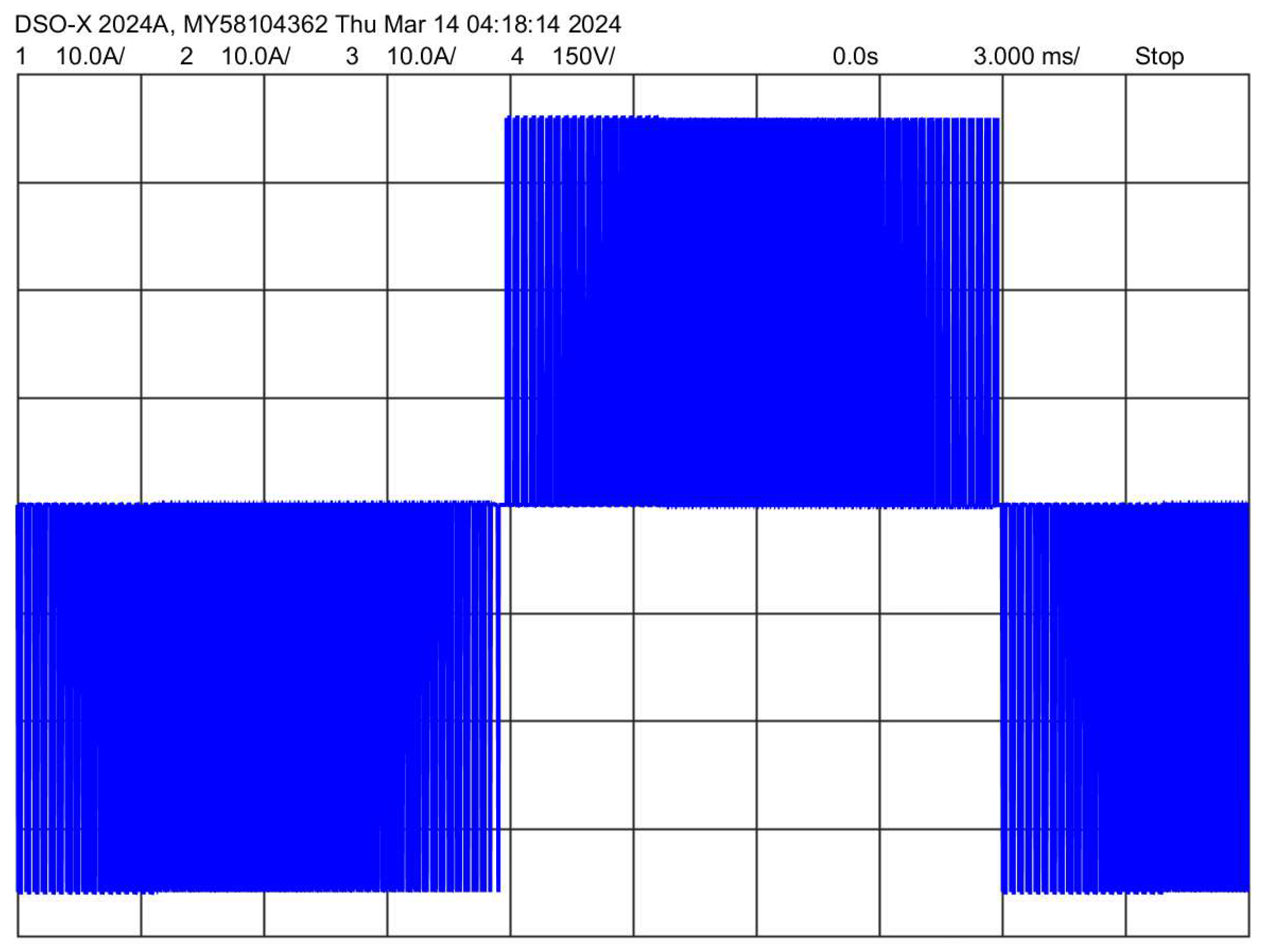
Figure 11.
Line voltage a-b around second 6.5 for DAPBC.
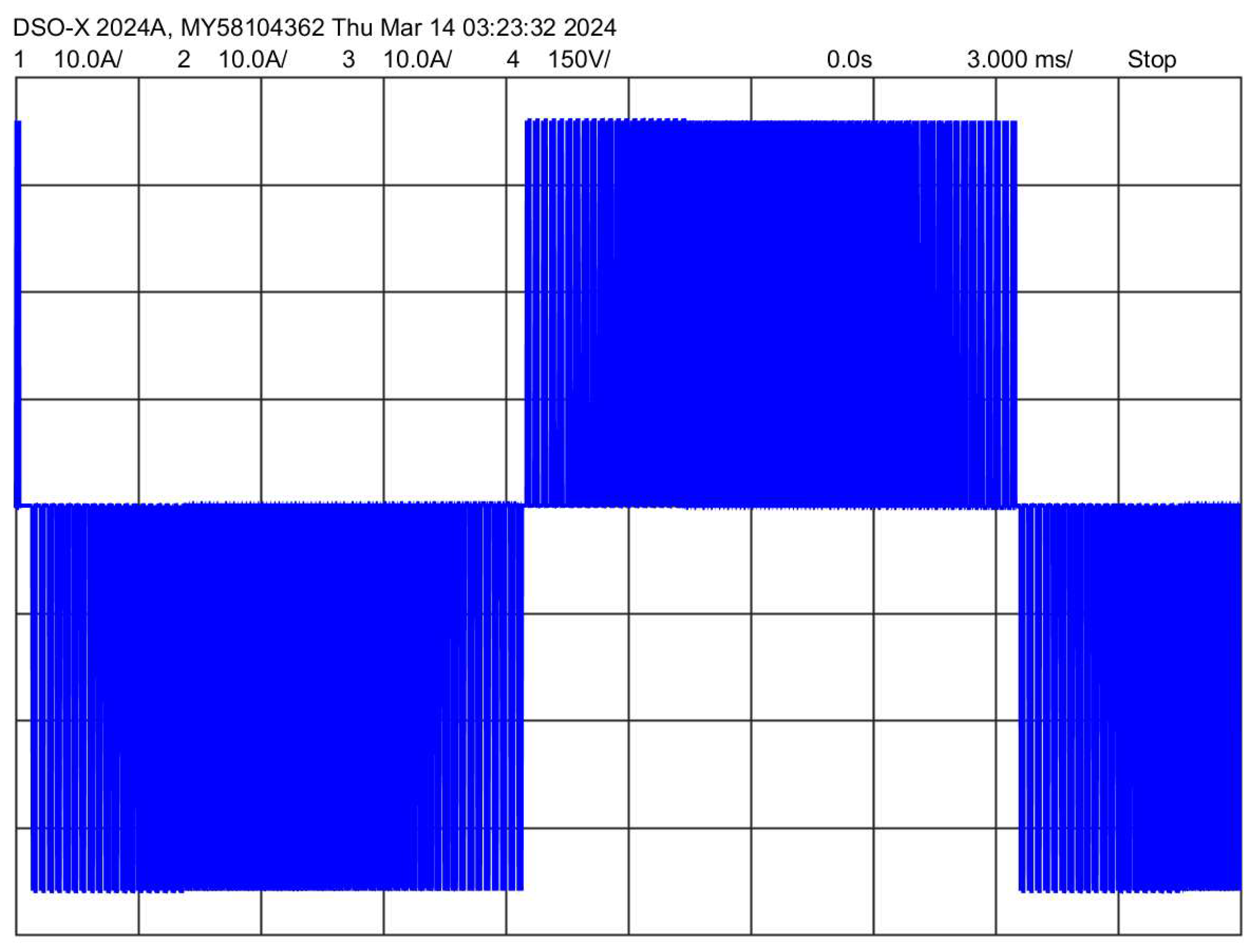
Figure 12.
Line voltage a-b around second 6.5 for the proposed CAPBC.


Table 1.
Comparative performance indexes for the rotor speed controllers.
| Tests | ||||||||||
|---|---|---|---|---|---|---|---|---|---|---|
| Performance Index | Time [s] | 2.0 | 2.5 | 3.0 | 3.5 | 4.0 | 5.0 | 6.0 | 7.0 | 9.0 |
| 1.00 | 1.00 | 1.00 | 1.00 | 1.00 | 1.00 | 1.00 | 0.80 | 1.10 | ||
| [% ] | 66.0 | 66.0 | 66.0 | 66.0 | 66.0 | 40.0 | 66.0 | 66.0 | 66.0 | |
| Speed [rad/s] | 25.0 | 60.0 | 85.0 | 120 | 152.36 | 150 | 152.36 | 152.36 | 152.36 | |
| Ess [%] (Ending) | PI | 0.1299 | 0.1212 | 0.1237 | 0.1189 | 0.0180 | 0.0307 | 0.0254 | 0.0243 | 0.0851 |
| DAPBC | 0.0850 | 0.0302 | 0.0804 | 0.0100 | 0.0063 | 0.0079 | 0.0195 | 0.0227 | 0.0468 | |
| CAPBC | 0.0512 | 0.0269 | 0.0659 | 0.0066 | 0.0029 | 0.0068 | 0.0190 | 0.0139 | 0.0171 | |
| MO [%] (Starting) | PI | 5.5983 | 10.6929 | 7.1124 | 5.3479 | 4.3302 | 4.1276 | 0.2338 | 2.7979 | 3.5007 |
| DAPBC | 3.5168 | 1.7019 | 1.1308 | 0.8651 | 0.7095 | 0.3595 | 0.2139 | 0.1751 | 0.3143 | |
| CAPBC | 3.4904 | 1.4038 | 0.8367 | 0.5941 | 0.4640 | 0.2938 | 0.1923 | 0.1663 | 0.1667 | |
| IAE [cm.s] | PI | 0.6491 | 0.6494 | 0.6501 | 0.6519 | 0.6541 | 0.6544 | 1.043 | 1.52 | 2.2654 |
| DAPBC | 0.0152 | 0.0198 | 0.0359 | 0.0368 | 0.0378 | 0.0529 | 0.0663 | 0.0694 | 0.1507 | |
| CAPBC | 0.0099 | 0.0059 | 0.0072 | 0.0102 | 0.0223 | 0.0356 | 0.0437 | 0.0452 | 0.1425 | |
| ISI [] | PI | 0.2785 | 0.2649 | 0.2656 | 0.2664 | 0.2672 | 0.3915 | 0.8797 | 1.1001 | 3.3045 |
| DAPBC | 0.2616 | 0.2619 | 0.2623 | 0.2625 | 0.2632 | 0.3907 | 0.8752 | 0.9837 | 3.3018 | |
| CAPBC | 0.2592 | 0.2594 | 0.2610 | 0.2624 | 0.2634 | 0.3900 | 0.8689 | 0.9729 | 3.3016 | |
Disclaimer/Publisher’s Note: The statements, opinions and data contained in all publications are solely those of the individual author(s) and contributor(s) and not of MDPI and/or the editor(s). MDPI and/or the editor(s) disclaim responsibility for any injury to people or property resulting from any ideas, methods, instructions or products referred to in the content. |
© 2024 by the authors. Licensee MDPI, Basel, Switzerland. This article is an open access article distributed under the terms and conditions of the Creative Commons Attribution (CC BY) license (https://creativecommons.org/licenses/by/4.0/).
Share and Cite
MDPI and ACS Style
Travieso-Torres, J.C.; Ricaldi-Morales, A.J.; Aguila-Camacho, N. Robust Combined Adaptive Passivity-Based Control for Induction Motors. Machines 2024, 12, 272. https://doi.org/10.3390/machines12040272
AMA Style
Travieso-Torres JC, Ricaldi-Morales AJ, Aguila-Camacho N. Robust Combined Adaptive Passivity-Based Control for Induction Motors. Machines. 2024; 12(4):272. https://doi.org/10.3390/machines12040272
Chicago/Turabian StyleTravieso-Torres, Juan Carlos, Abdiel Josadac Ricaldi-Morales, and Norelys Aguila-Camacho. 2024. "Robust Combined Adaptive Passivity-Based Control for Induction Motors" Machines 12, no. 4: 272. https://doi.org/10.3390/machines12040272
Note that from the first issue of 2016, this journal uses article numbers instead of page numbers. See further details here.