RBF-Based Fractional-Order SMC Fault-Tolerant Controller for a Nonlinear Active Suspension

Abstract

Active suspension control technologies have become increasingly significant in improving suspension performance for driving stability and comfort. An RBF-based fractional-order SMC fault-tolerant controller is developed in this research to guarantee ride comfort and handling stability when faced with the partial loss of actuator effectiveness due to failure. To obtain better control performance, fractional-order theory and the RBF algorithm are discussed to solve the jitter vibration problem in SMC, and the RBF is exploited to obtain a more appropriate switching gain. First, a half-nonlinear active suspension model and a fault car model are presented. Then, the design process of the RBF-based fractional-order SMC fault-tolerant controller is described. Next, a simulation is presented to demonstrate the effectiveness of the proposed strategy. According to the simulation, the proposed method can improve performance in the case of a healthy suspension, and the fault-tolerant controller can guarantee the capabilities when actuators go wrong.

1. Introduction

Suspension systems are significant elements in modern cars [1]. Suspension systems can be categorized into three groups according to the mold of the dampers [2]: passive, semi-active, and active suspension systems. Unlike the passive and semi-active forms, there are active actuators that generate active force, which can elevate their properties to a great extent [3].

With constant technological improvement, on the one hand, a wide variety of sensors are used in suspension systems to monitor the conditions of roads and the movement of vehicles. On the other hand, plentiful control solutions have been applied in control mechanisms. Based on the aforementioned circumstances, a car can maintain optimal balance and control due to active control technology, which lessens shocks and vibrations and enhances ride stability and comfort for the occupants.

Therefore, the control strategy for active suspension has become a hot research topic. Today, active suspension systems are widely used in automobiles. In [4], an MPC control technology was used in air suspension systems equipped with a multi-mode switching damper. The authors of [5] presented the $H_{\infty }$ control method under constrained conditions. The authors of [6] presented a hybrid $H_2$ and $H_{\infty }$ control algorithm for active suspension. In [7], a multi-complex model based on predictive control was presented. Ref. [8] presented a multi-agent approach for active steering and active suspension. For time-varying parameter uncertainty, a robust infinity control method is discussed [9].

The linear suspension system is the main topic of traditional studies. However, springs and dampers in suspension systems display some nonlinear characteristics, and their precise manifestations are unexpected. As a result, suspension systems are typical nonlinear systems. When the initial nonlinearity of suspension systems is ignored, this can bring about a worse impact on the control effect and significantly reduce the model’s accuracy [10]. Therefore, nonlinear models serve as the foundation for research with significant practical value.

It is worth noting that the majority of the studies mentioned above were based on the assumption that a suspension system can work at its best; therefore, all of the results stated above are consistent with the premise that every system’s control component is running at its best.

However, vehicle suspension systems are intricate and made up of mechanical, electronic, and other components. As the amount of time spent working rises, certain other unsetting elements can lead to the failure of suspension systems and actuators. In addition, system procedures are highly difficult due to the inherent uncertainties of active suspension systems. Common failures that happen to the actuator consist of gain variation, constant deviation, and seizure failure [11,12].

When a common failure of an actuator occurs, traditional controllers cannot perform better. Active suspension systems are sensitive and prone to faults due to their sophisticated design and demanding operating circumstances, which could result in the system performing poorly or failing. To guarantee the control effect when actuator failure occurs, fault-tolerant controllers have been designed. Fault tolerance can ensure the stability of a suspension. Fault-tolerant control techniques that can make up for a failure and keep a closed-loop system operating at a satisfactory rate have been the focus of numerous studies in recent years due to their theoretical and practical significance.

The difficulties rest with reliable fault-tolerant control. Therefore, the design of reliable fault-tolerant controllers has been a topic of extensive study. For example, in [13], a sliding-mode control method was presented for a linear active suspension with sensor and actuator faults. A reliable fuzzy-based robust feedback strategy was discussed for a vehicle suspension with actuator faults [14]. The authors of [15] discussed a robust fault-tolerant controller for active suspension systems with finite frequency constraints. A fuzzy-based fault-tolerant controller was discussed for an electromagnetic system [16]. In [17], a feedback-observer-based fault-tolerant controller was presented for active suspension systems.

Sliding-mode control (SMC) is a unique form of nonlinear control that is extremely resilient to uncertain models and disturbances. In addition, SMC is a specific type of nonlinear control method and is extremely resilient to parameter uncertainty and perturbations outside the model [18]. Numerous studies have used sliding-mode control in active controlling problems. In [19], a PID-based SMC controller was designed. In [20], an SMC fault-tolerant controller was used to ensure the suspension performance with actuator failure.

In real systems, sliding-mode control generates high-frequency vibration, and this jittering vibration can affect the accuracy of the system or even destroy it, which affects the control effectiveness of the system. Therefore, scholars have focused their attention on solving the jittering vibration problem of SMC.

However, it is not influenced by changes in control object parameters and the interference of external conditions, and it has very good robustness. Therefore, the jitter vibration problem of sliding-mode control cannot be eliminated but only attenuated. Currently, the commonly used methods are the boundary layer method [21,22], the adjustment of the convergence law [23], and intelligent technology methods.

For example, the authors of [24] designed a hybrid controller by combining fuzzy control and a sliding-mode approach. For better robustness, global optimality, feasibility, and high efficiency in solving nonlinear problems with high optimization performance, genetic algorithms (GAs) are used in SMC [25]. Particle swarm optimization (PSO) is also used in SMC to enhance the control effect [26]. In addition, there are sector characterization approaches, filtering approaches, observer approaches, and so on [27]. The existing research results show that the use of the fractional-order control strategy is better than the integer-order control strategy [28]. Based on fractional-order theory, the fractional order is used in SMC to reduce the jitter vibration problem.

In addition, the switching gain in SMC also affects the control effect and can cause a jitter vibration problem.

RBF neural networks have a strong self-learning function and a strong ability to transfer to nonlinear systems. It is possible to approximate the model information of a controlled object and the imposed disturbance using the neural network’s universal approximation property, and with the help of the neural network’s adaptive weight adjustments, it is possible to achieve adaptive neural fully naked sliding-mode control without the use of model information.

Consequently, in this study, an RBF-based fractional-order SMC fault-tolerant controller was developed to improve ride comfort and handling stability under the partial loss of actuator effectiveness due to a fault. Fractional-order theory and the RBF method are used to reduce the jitter vibration. The RBF neural network is also used to obtain a more appropriate switching gain for SMC.

The main contributions of this study are summarized as follows: Section 2 gives the road profile model, nonlinear half-car vehicle model, and fault system model. In Section 3, an RBF-based fractional-order SMC fault-tolerant controller is presented (FRSMC and FRFTC). Section 4 provides the simulation results. To better illustrate the validity of the methodology proposed in this study, it is compared with the genetic algorithm-based SMC method (GASMC) in the case of no actuator failure. A particle-swarm-optimization-based SMC fault-tolerant controller (PSFTC) is compared with the proposed algorithm in the case of actuator failure. Section 5 concludes the paper.

2. Problem Formulation

2.1. Road Disturbance

When referring to the study of suspension control, the road input should be considered first. When traveling through rough terrain, a car will generate vibration. Studies have commonly adopted two input forms: the random and impact versions. In this study, the most prevalent random road profile is applied. ISO/TC108/SC2N67 [29] recommends using the power spectral density function to simulate pavement unevenness. In this study, a random road input model is represented by the integration of white noise signals. The random road input model is expressed as follows:

$${\dot{x}}_g\left(t\right)=2\pi f_0{x}_g\left(t\right)+2\pi w\left(t\right)\sqrt{G_{0}v}$$

(1)

where

$q\left(t\right)$	road profile;
$w\left(t\right)$	random white noise signal;
$f_0=0.01$	low cut-off frequency;
$G_0=64\times {10}^{-6}$	road roughness;
v = 60 km/h	vehicle speed.

To make the model of the constructed pavement inputs more realistic, the inputs from the rear wheels can be viewed as a time delay of the input signals from the front wheels. The time delay can be expressed as

$$t=\frac{a+b}{v}$$

(2)

Here, a and b are the front and rear distances from the front and rear wheels to the center of the car body. Figure 1 and Figure 2 show random road disturbances.

2.2. Nonlinear Active Suspension System Model

To study the vertical vibration, pitching motion, and coupled vertical and pitching motion of a car, a half-vehicle model is usually utilized, and left–right symmetry is usually assumed to simplify the analysis. Therefore, in this study, a half-car suspension model is used. The half-car model has simplicity and the capacity to precisely describe the essential components. The nonlinear half-car model is shown in Figure 3.

The meanings of the variable parameters used in the model are as follows:

$m_s$	car body mass;
$m_1\&m_2$	unsprung mass of the front and rear;
I	pitch moment of inertia;
$\phi$	pitch angle;
$x_{s1}\&x_{s2}$	front and rear body displacement;
$x_{u1}\&x_{u2}$	front and rear unsprung mass displacement;
$x_{g1}\&x_{g2}$	front and rear road inputs;
$a\&b$	distance of suspension from the center mass of the vehicle body;
$F_{s1}\&F_{s2}$	front and rear nonlinear spring force;
$F_{d1}\&F_{d2}$	front and rear nonlinear damper force;
$u_1\&u_2$	front and rear active force;
$F_{t1}\&F_{t2}$	front and rear elastic force of the tire.

The parameters of the dampers, springs, and tires in an actual suspension are significantly nonlinear, but the linear model is usually used in research, resulting in some errors in the results, so this study adopts a nonlinear suspension.

The dynamic equations used to describe the half-car suspension model are established as follows:

$$\left\{\begin{array}{c}m{\ddot{x}}_s=F_{s1}+F_{s2}+F_{d1}+F_{d2}+u_1+u_2\hfill \\ I\ddot{\phi }=b\left(F_{s2}+F_{d2}+u_2\right)-a\left(F_{s1}+F_{d1}+u_1\right)\hfill \\ m_1{\ddot{x}}_{u1}=-F_{s1}-F_{d1}-u_1+F_{t1}\hfill \\ m_2{\ddot{x}}_{u2}=-F_{s2}-F_{d2}-u_2+F_{t2}\hfill \end{array}\right.$$

(3)

The dynamic functions of the nonlinear and linear springs and dampers are established as follows:

$$\left\{\begin{array}{c}{F}_{s1}=k_s(x_{s1}-x_{u1})+k_{sn}{(x_{s1}-x_{u1})}^3\hfill \\ F_{s2}=k_s(x_{s2}-x_{u2})+k_{sn}{(x_{s2}-x_{u2})}^3\hfill \\ F_{d1}=c_s({\dot{x}}_{s1}-{\dot{x}}_{u1})+c_{sn}{({\dot{x}}_{s1}-{\dot{x}}_{u1})}^2\hfill \\ F_{d2}=c_s({\dot{x}}_{s2}-{\dot{x}}_{u2})+c_{sn}{({\dot{x}}_{s2}-{\dot{x}}_{u2})}^2\hfill \\ F_{t1}=k_t(x_{u1}-x_{g1})\hfill \\ F_{t2}=k_t(x_{u2}-x_{g2})\hfill \end{array}\right.$$

(4)

where

$k_s\&k_{sn}$	linear and nonlinear spring stiffness;
$c_s\&c_{sn}$	linear and nonlinear damping coefficients;
$k_t\&c_t$	spring stiffness coefficient and damping coefficient of the tire.

Let

$$\left\{\begin{array}{c}{f}_1(x_s\left(t\right)-x_u\left(t\right))=[k_{sn}{(x_{s1}-x_{u1})}^3,k_{sn}{(x_{s2}-x_{u2})}^3]\hfill \\ f_2(x_s\left(t\right)-x_u\left(t\right))=[c_{sn}{({\dot{x}}_{s1}-{\dot{x}}_{u1})}^2,c_{sn}{({\dot{x}}_{s2}-{\dot{x}}_{u2})}^2]\hfill \end{array}\right.$$

(5)

$M_s=\left[\begin{array}{cc}{m}_s& 0\\ 0& I\end{array}\right]$; $M_u=\left[\begin{array}{cc}{m}_1& 0\\ 0& m_2\end{array}\right]$; $C_s=\left[\begin{array}{cc}{c}_s& 0\\ 0& c_s\end{array}\right]$; $K_s=\left[\begin{array}{cc}{k}_s& 0\\ 0& k_s\end{array}\right]$; $K_t=\left[\begin{array}{cc}{k}_t& 0\\ 0& k_t\end{array}\right]$;

$G=\left[\begin{array}{cc}1& 1\\ -a& b\end{array}\right]$; $f\left(t\right)=\left[\begin{array}{cc}{f}_1{(x_s\left(t\right)-x_u\left(t\right))}^T& f_2{({\dot{x}}_s\left(t\right)-{\dot{x}}_u\left(t\right))}^T\end{array}\right].$

Then, the suspension system’s dynamic function (3) can be rewritten as Equation (6):

$$\left\{\begin{array}{c}{M}_s\ddot{q}\left(t\right)=G{K}_s\left(x_s\left(t\right)-x_u\left(t\right)\right)+G{C}_s\left({\dot{x}}_s\left(t\right)-{\dot{x}}_u\left(t\right)\right)+Gf(x,t)+Gu\left(t\right)\hfill \\ M_u{\ddot{x}}_u\left(t\right)=-G{K}_s\left(x_s\left(t\right)-x_u\left(t\right)\right)-G{C}_s\left({\dot{x}}_s\left(t\right)-{\dot{x}}_u\left(t\right)\right)-Gf(x,t)-Gu\left(t\right)\hfill \\ +K_t\left(x_u\left(t\right)-x_g\left(t\right)\right)\hfill \end{array}\right.$$

(6)

where

$$\left\{\begin{array}{cc}\hfill q\left(t\right)& ={[x_s\left(t\right),\phi \left(t\right)]}^T;\hfill \\ \hfill x_s\left(t\right)& ={[x_{s1}\left(t\right),x_{s2}\left(t\right)]}^T\hfill \\ \hfill x_u\left(t\right)& ={[x_{u1}\left(t\right),x_{u2}\left(t\right)]}^T;\hfill \\ \hfill x_s\left(t\right)& ={[x_{s1}\left(t\right),x_{s2}\left(t\right)]}^T;\hfill \\ \hfill u\left(t\right)& ={[u_1\left(t\right),u_2\left(t\right)]}^T;\hfill \\ \hfill f(x,t)& =[k_{sn}{(x_s\left(t\right)-x_u\left(t\right))}^T,c_{sn}{({\dot{x}}_s\left(t\right)-{\dot{x}}_u\left(t\right))}^T].\hfill \end{array}\right.$$

(7)

The state variables are defined as follows:

$$x\left(t\right)={\left[\begin{array}{cccc}{(x_s\left(t\right)-x_u\left(t\right))}^T& {\dot{x}}_s\left(t\right)& {(x_u\left(t\right)-x_g\left(t\right))}^T& {\dot{x}}_u\left(t\right)\end{array}\right]}^T$$

(8)

The disturbance road input variables are defined as follows:

$$w\left(t\right)={\left[\begin{array}{cc}{x}_{g1}\left(t\right)\hfill & x_{g2}\left(t\right)\end{array}\right]}^T$$

(9)

The control input variables are defined as follows:

$$u\left(t\right)={\left[\begin{array}{cc}{u}_1\left(t\right)\hfill & u_2\left(t\right)\end{array}\right]}^T$$

(10)

The output variables are defined as follows:

$$y\left(t\right)={\left[\begin{array}{cccc}\ddot{q}\left(t\right)\hfill & {(x_s\left(t\right)-x_u\left(t\right))}^T& K_t\times {(x_u\left(t\right)-x_g\left(t\right))}^T& x_u\left(t\right)\end{array}\right]}^T$$

(11)

For easier calculations, we suppose the following:

• Wheels have ideal terrain signals;
• The pitch angle $\phi$ is small.

The front and rear suspension displacements can be rewritten as in Equation (12):

$$\left\{\begin{array}{c}{x}_{s1}\cong x_s-asin\phi \approx x_s-a\phi \hfill \\ x_{s2}\cong x_s+asin\phi \approx x_s+b\phi \hfill \end{array}\right.$$

(12)

Then, the state-space function of the half-car suspension system model is established in the form of Equation (13):

$$\left\{\begin{array}{c}\dot{x}\left(t\right)=Ax\left(t\right)+B_{1}w\left(t\right)+B_{2}u\left(t\right)+F_{1}f(x,t)\hfill \\ y\left(t\right)=Cx\left(t\right)+Du\left(t\right)+F_{2}f(x,t)\hfill \end{array}\right.$$

(13)

where

$\mathbf{A}=\left[\begin{array}{cccc}{\mathbf{0}}^{\mathbf{2}\times \mathbf{2}}& {\mathbf{I}}^{\mathbf{2}\times \mathbf{2}}& {\mathbf{0}}^{\mathbf{2}\times \mathbf{2}}& -{\mathbf{I}}^{\mathbf{2}\times \mathbf{2}}\\ {\mathbf{G}}^{\mathbf{T}}{{\mathbf{M}}_{\mathbf{s}}}^{-\mathbf{1}}\mathbf{G}{\mathbf{K}}_{\mathbf{s}}& {\mathbf{G}}^{\mathbf{T}}{{\mathbf{M}}_{\mathbf{s}}}^{-\mathbf{1}}\mathbf{G}{\mathbf{C}}_{\mathbf{s}}& {\mathbf{0}}^{\mathbf{2}\times \mathbf{2}}& {\mathbf{G}}^{\mathbf{T}}{{\mathbf{M}}_{\mathbf{s}}}^{-\mathbf{1}}\mathbf{G}{\mathbf{C}}_{\mathbf{s}}\\ {\mathbf{0}}^{\mathbf{2}\times \mathbf{2}}& {\mathbf{0}}^{\mathbf{2}\times \mathbf{2}}& {\mathbf{0}}^{\mathbf{2}\times \mathbf{2}}& {\mathbf{I}}^{\mathbf{2}\times \mathbf{2}}\\ -{{\mathbf{M}}_{\mathbf{u}}}^{-\mathbf{1}}{\mathbf{K}}_{\mathbf{s}}& -{{\mathbf{M}}_{\mathbf{u}}}^{-\mathbf{1}}{\mathbf{C}}_{\mathbf{s}}& {{\mathbf{M}}_{\mathbf{u}}}^{-\mathbf{1}}{\mathbf{K}}_{\mathbf{u}}& {{\mathbf{M}}_{\mathbf{u}}}^{-\mathbf{1}}{\mathbf{C}}_{\mathbf{s}}\end{array}\right];$

${\mathbf{B}}_{\mathbf{1}}=\left[\begin{array}{c}{\mathbf{0}}^{\mathbf{2}\times \mathbf{2}}\\ {\mathbf{0}}^{\mathbf{2}\times \mathbf{2}}\\ -{\mathbf{I}}^{\mathbf{2}\times \mathbf{2}}\\ {\mathbf{0}}^{\mathbf{2}\times \mathbf{2}}\end{array}\right];{\mathbf{B}}_{\mathbf{2}}=\left[\begin{array}{c}\mathbf{0}\\ {\mathbf{G}}^{\mathbf{T}}{{\mathbf{M}}_{\mathbf{s}}}^{-\mathbf{1}}\mathbf{G}\\ \mathbf{0}\\ -{{\mathbf{M}}_{\mathbf{u}}}^{-\mathbf{1}}\end{array}\right];{\mathbf{F}}_{\mathbf{1}}=\left[\begin{array}{c}{\mathbf{0}}^{\mathbf{2}\times \mathbf{2}}\\ {\mathbf{G}}^{\mathbf{T}}{{\mathbf{M}}_{\mathbf{s}}}^{-\mathbf{1}}\mathbf{G}\\ {\mathbf{0}}^{\mathbf{2}\times \mathbf{2}}\\ -{\mathbf{G}}^{\mathbf{T}}{{\mathbf{M}}_{\mathbf{s}}}^{-\mathbf{1}}\mathbf{G}\end{array}\right];$

$\mathbf{C}=\left[\begin{array}{cccc}{\mathbf{G}}^{\mathbf{T}}{{\mathbf{M}}_{\mathbf{s}}}^{-\mathbf{1}}\mathbf{G}{\mathbf{K}}_{\mathbf{s}}& {\mathbf{G}}^{\mathbf{T}}{{\mathbf{M}}_{\mathbf{s}}}^{-\mathbf{1}}\mathbf{G}{\mathbf{C}}_{\mathbf{s}}& {\mathbf{0}}^{\mathbf{2}\times \mathbf{2}}& -{\mathbf{G}}^{\mathbf{T}}{{\mathbf{M}}_{\mathbf{s}}}^{-\mathbf{1}}\mathbf{G}{\mathbf{C}}_{\mathbf{s}}\\ \mathbf{I}& {\mathbf{0}}^{\mathbf{2}\times \mathbf{2}}& {\mathbf{0}}^{\mathbf{2}\times \mathbf{2}}& {\mathbf{0}}^{\mathbf{2}\times \mathbf{2}}\\ {\mathbf{0}}^{\mathbf{2}\times \mathbf{2}}& {\mathbf{0}}^{\mathbf{2}\times \mathbf{2}}& {\mathbf{0}}^{\mathbf{2}\times \mathbf{2}}& {\mathbf{K}}_{\mathbf{t}}\end{array}\right];$

$\mathbf{D}=\left[\begin{array}{c}{{\mathbf{M}}_{\mathbf{s}}}^{-\mathbf{1}}\mathbf{G}\\ \mathbf{0}\\ \mathbf{0}\end{array}\right];{\mathbf{F}}_{\mathbf{2}}=\left[\begin{array}{c}{{\mathbf{M}}_{\mathbf{s}}}^{-\mathbf{1}}\mathbf{G}\\ \mathbf{0}\\ \mathbf{0}\end{array}\right].$

2.3. Nonlinear Active Suspension System Fault Model

We should note that the established dynamic equations are built on the ideal conditions, which means that all of the components can work normally. However, there are numerous electronic and mechanical elements. As the working time increases, some other disturbing factors may cause failures in suspension systems and actuators. In addition, active suspension systems’ inescapable uncertainties also make the system process extremely challenging. Common failures that happen to the actuator consist of gain variation, constant deviation, and seizure failure. When the suspension components fail to work normally, the actuator cannot produce the desired active force. The suspension cannot run as it is supposed to.

The common actuator faults, such as constant deviation or offset, were first investigated on the experiment bench before being modeled in the finite parameter family as a constraint gain or drift. Furthermore, continuous deviation can be seen as time-varying gain defects. Without sacrificing generality, the gain faults were employed to characterize the actuator fault model [30,31]. In this study, gain variation in the actuator is considered.

In the fault suspension model, the force $u{f}_j$ has the following presentation:

$$u{f}_j=\delta u_j$$

(14)

$u_f$	active force produced by the fault actuator;
j	the jth actuator;
$\delta$	the effectiveness factor;
$\delta =0$	the actuator cannot work anymore;
$\delta =1$	the actuator can work normally;
$0<\delta <1$	partial loss in the actuator.

Let

$$M=\left[\begin{array}{cc}{\delta }_1& 0\\ 0& {\delta }_2\end{array}\right]$$

(15)

$$u_f\left(t\right)=Mu\left(t\right)$$

(16)

Then, the state-space function of the suspension system fault model is established as follows:

$$\left\{\begin{array}{c}\dot{x}\left(t\right)=Ax\left(t\right)+B_{1}w\left(t\right)+B_{2}Mu\left(t\right)+F_{1}f(x,t)\hfill \\ y\left(t\right)=Cx\left(t\right)+DMu\left(t\right)+F_{2}f(x,t)\hfill \end{array}\right.$$

(17)

3. Fault-Tolerant Controller Design

An RBF-based fractional-order SMC fault-tolerant controller for a nonlinear active suspension is designed in this section.

3.1. Fractional-Order Sliding-Mode Control Method

There are three different definitions of fractional-order calculus: Granwald–Leikov (GL), Reimann–Liouville (RL), and Caputo [32]. The Caputo method is used in this research and is shown in the following equation:

$${}_a{}^{ }D_t^{\alpha }f\left(t\right)=\frac{1}{\Gamma (1-\gamma )}{\int }_a^t\frac{f^{(m+1)}\left(\tau \right)}{{(t-\tau )}^{\gamma }}d\tau$$

(18)

where $\alpha =m+\gamma$, m is an integer, $0<\gamma \le 1$, and $\Gamma$ is the Gamma function.

The Laplace transform of the Caputo expression can be written as

$$L\left\{{}_a{}^{C}D_t^{\alpha }f\left(t\right)\right\}=s^{\alpha }F\left(s\right)-\sum _{k=0}^{n-1}{s}^{(\alpha -k-1)}{f}^{\left(k\right)}\left(0\right)$$

(19)

When the initial condition is 0,

$$L\left\{\frac{d^{\alpha }f\left(t\right)}{d{t}^{\alpha }}\right\}=s^{\alpha }L\left\{f\left(t\right)\right\}$$

(20)

In this study, the error between the actual model and the reference model of the body mass velocity and displacement is selected as the sliding switch surface. The sliding switch surface is shown in Equation (21):

$$S\left(e\right)=\lambda e+D^{\alpha }\dot{e}$$

(21)

where $\lambda >0$ is the gain of the sliding switch surface and $D^{\alpha }$ is the fractional-order operator. $0<\alpha <1$ represents the $\alpha$-order integral.

The variables of the nonlinear suspension system error are chosen in the manner described below [33]:

$$\left\{\begin{array}{cc}\hfill e_1& =x_s-r_1\hfill \\ \hfill e_2& ={\dot{x}}_s-r_2\hfill \end{array}\right.$$

(22)

Here, $r_1$ is the ideal signal of $x_s$. $r_2$ is the ideal signal of ${\dot{x}}_s$. The goal of the control is for the system vibration signal to converge to zero. Hence, the ideal signal is zero.

We take the derivative of the error variables as follows:

$$\left\{\begin{array}{cc}\hfill {\dot{e}}_1& ={\dot{x}}_s-{\dot{r}}_1=e_2+r_2-{\dot{r}}_1\hfill \\ \hfill {\dot{e}}_2& ={\ddot{x}}_s-{\dot{r}}_2=\frac{1}{m_s}\left(F_{s1}+F_{s2}+F_{d1}+F_{d2}\right)+\frac{1}{m_s}\left(u_1+u_2\right)-{\dot{r}}_2=f\left(x\right)+\frac{1}{m_s}u-{\dot{r}}_2\hfill \end{array}\right.$$

(23)

The sliding-mode surface is derived as follows:

$$\begin{array}{cc}\hfill \dot{S}\left(e\right)& =\lambda {\dot{e}}_1+D^{\alpha }{\ddot{e}}_1\hfill \\ \hfill & =\lambda (e_2+r_2-{\dot{r}}_1)+D^{\alpha }\left[f\left(x\right)+\frac{1}{m_s}u-{\ddot{r}}_1\right]\hfill \end{array}$$

(24)

The equivalent control law is defined as follows:

$$u_{eq}=m_s\left[-\lambda D^{-\alpha }(e_2+r_2-{\dot{r}}_1)-f\left(x\right)+{\ddot{r}}_1\right]$$

(25)

The convergence law is defined as follows:

$$\dot{S}\left(e\right)=-\epsilon S-K_0\mathrm{sgn}\left(\mathrm{s}\right)$$

(26)

where $\epsilon >0$, $K_0>0$. $\mathrm{sgn}\left(\mathrm{s}\right)$ is the symbol function, and $\mathrm{sgn}\left(\mathrm{s}\right)$ is shown in the following equation:

$$\mathrm{sgn}\left(\mathrm{s}\right)=\left\{\begin{array}{cc}1& \mathrm{s}>0\\ 0& \mathrm{s}=0\\ -1& \mathrm{s}<0\end{array}\right.$$

(27)

Then, the fault-tolerant controller is expressed in Equation (28):

$$u=m_s\left[D^{-\alpha }\left[-\lambda ({\dot{x}}_s-{\dot{r}}_1)\right]-f\left(x\right)+{\ddot{r}}_1\right]-\epsilon S-K_0\mathrm{sgn}\left(\mathrm{s}\right)$$

(28)

To decrease the jitter, the saturation function $sat(s/\Phi )$ is used to replace the symbol function $\mathrm{sgn}\left(\mathrm{s}\right)$:

$$u=m_s\left[D^{-\alpha }\left[-\lambda ({\dot{x}}_s-{\dot{r}}_1)\right]-f\left(x\right)+{\ddot{r}}_1\right]-\epsilon S-K_{0}sat(s/\Phi )$$

(29)

where $sat(s/\Phi )=\left\{\begin{array}{cc}\mathrm{sgn}(s/\Phi )& |s/\Phi |\ge 1\\ s/\Phi & |s/\Phi |<1\end{array}\right.$, $\Phi >0$ is the critical width, and $K_0$ is the switching gain.

Equation (29) can be rewritten as Equation (30):

$$\left[\begin{array}{cc}1& 1\end{array}\right]\left[\begin{array}{c}{u}_1\\ u_2\end{array}\right]=\left[\begin{array}{cc}1& 1\end{array}\right]\left[\begin{array}{c}\frac{b}{a+b}\times m_s\left[D^{-\alpha }\left[-\lambda ({\dot{x}}_s-{\dot{r}}_1)\right]-f\left(x\right)+{\ddot{r}}_1\right]-\epsilon S-k_{1}sat(s/\Phi )\\ \frac{a}{a+b}\times m_s\left[D^{-\alpha }\left[-\lambda ({\dot{x}}_s-{\dot{r}}_1)\right]-f\left(x\right)+{\ddot{r}}_1\right]-\epsilon S-k_{2}sat(s/\Phi )\end{array}\right]$$

(30)

Let

$$\left\{\begin{array}{cc}\hfill u_1& =\frac{b}{a+b}\times m_s\left[D^{-\alpha }\left[-\lambda ({\dot{x}}_s-{\dot{r}}_1)\right]-f\left(x\right)+{\ddot{r}}_1)\right]-\epsilon S-k_{1}sat(s/\Phi )\hfill \\ \hfill u_2& =\frac{a}{a+b}\times m_s\left[D^{-\alpha }\left[-\lambda ({\dot{x}}_s-{\dot{r}}_1)\right]-f\left(x\right)+{\ddot{r}}_1\right]-\epsilon S-k_{2}sat(s/\Phi )\hfill \end{array}\right.$$

(31)

$$K=\left[\begin{array}{c}{k}_1\\ k_2\end{array}\right],K_0=k_1+k_2$$

(32)

3.2. RBF-Based Fractional-Order SMC Fault-Tolerant Controller

RBF is a type of intelligence method, and many researchers have used it in control engineering. The structure of RBF is usually made up of input, hidden, and output layers.

An RBF neural network simulates the human brain’s ability to respond locally and interweave with other overlays. It can optimally approximate arbitrary continuous functions at a very fast learning rate. It has a simple structure and is capable of local approximation without local minima.

RBF is used to reduce the jitter vibration and obtain the optimal switching gain. Generally speaking, the optimization of SMC using RBF is divided into two forms:

• Optimizing the equivalent control of SMC;
• Optimizing the toggle switch of SMC.

The method used in this study is the optimization of the toggle switch of sliding-mode control. According to the real-time dynamic state, the toggle switch is adjusted. The RBF is employed to obtain the optimal switching gain K. According to the theory, the output of the RBF neural network is the switching gain K. The logic structure of RBF is presented in Figure 4.

$x={[x_1,x_2]}^T={[s,\dot{s}]}^T$ is the input of RBF. The output y can be obtained with Equation (33):

$$y\left(t\right)=w\times h=\left|\sum _{j=1}^3{w}_j\times h_j\right|=k$$

(33)

where $w={\left[w_1,w_2,w_3\right]}^T$ is the weight vector of the RBF neural network and $h=\left[h_1,h_2,h_3\right]$ is the output of the hidden layer.

In the hidden layer, for the RBF, the Gaussian function is selected. The RBF-based strategy is displayed in the following:

$$h_j=exp\left(-\frac{{∥x-c_j∥}^2}{b_j^2}\right)$$

(34)

where $c_j=\left[c_1,c_2,c_3\right]$ is the neural network center vector. $b_j=\left[b_1,b_2,b_3\right]$ is the basis width vector.

According to the SMC theory and neural network approximation properties, as the system approaches convergence, the control goal is $s\dot{s}\to 0$. Therefore, let $E=s\left(t\right)\dot{s}\left(t\right)$; then, the weighting parameters can be expressed in the form of Equation (35):

$$d{w}_j=-\eta \frac{\partial E}{\partial w_j\left(t\right)}=-\eta \frac{\partial s\left(t\right)\partial \dot{s}\left(t\right)}{\partial w_j\left(t\right)}=-\eta \frac{\partial s\left(t\right)\partial \dot{s}\left(t\right)}{\partial k}\frac{\partial k}{\partial w_j\left(t\right)}$$

(35)

where $\eta >0$ for

$$\frac{\partial s\left(t\right)\partial \dot{s}\left(t\right)}{\partial w_j\left(t\right)}=s\left(t\right)\frac{\partial \dot{s}\left(t\right)}{\partial k}=-bs\left(t\right)$$

(36)

Then,

$$\frac{\partial k}{\partial w_j\left(t\right)}=exp\left(-\frac{{∥x-c_j∥}^2}{2{b_j}^2}\right)$$

(37)

By substituting Equations (35) and (36) into Equation (37), Equation (38) can be obtained:

$$d{w}_j=\eta ·b·s\left(t\right)·exp\left(-\frac{{∥x-c_j∥}^2}{2{b_j}^2}\right)=\eta ·b·s\left(t\right)·h_j$$

(38)

The Gaussian function of the basis width can be expressed in the form of Equation (39):

$$d{b}_j=-\eta \frac{\partial E}{\partial b_j}=\eta bs\left(t\right)\frac{{∥x-c_j∥}^2}{2{b_j}^3}$$

(39)

The parameters of the central node in the hidden layer are shown in (40):

$$d{c}_j=-\eta \frac{\partial E}{\partial c_j}=\eta bs\left(t\right)w_j{h}_j\frac{x-c_j}{{b_j}^2}$$

(40)

Therefore, the neural network weights are updated as described by Equation (41):

$$\left\{\begin{array}{cc}\hfill w_j\left(t\right)& =w_j(t-1)+d{w}_j\left(t\right)+\eta \left(w_j(t-1)-w_j(t-2)\right)\hfill \\ \hfill b_j\left(t\right)& =b_j(t-1)+d{b}_j\left(t\right)+\eta \left(b_j(t-1)-b_j(t-2)\right)\hfill \\ \hfill c_j\left(t\right)& =c_j(t-1)+d{c}_j\left(t\right)+\eta \left(c_j(t-1)-c_j(t-2)\right)\hfill \end{array}\right.$$

(41)

Finally, the controller structure is presented in Figure 5.

Here, $E_0=\frac{1}{2}\sqrt{{e_1}^2+{e_2}^2}$, $E_n$ is the given precision. When $E_0<E_n$, the optimal switching gain can be obtained.

The detailed steps are as follows:

• Step 1 Calculating the sliding switch surface: Equation (21);
• Step 2 Obtaining the switching gain: Equations (33)–(41);
• Step 3 Obtaining the active force expression: Equation (31);
• Step 4 Simulation: Equation (17);
• Step 5 Calculating $E_0$: If $E_0<E_n$, then output; if $E_0\ge E_n$, then return to step 1.

3.3. Stability of the Control System

The Lyapunov function [34] is chosen as described by Equation (42):

$$V=\frac{1}{2}{s}^2$$

(42)

By taking the derivative, we can obtain Equation (43):

$$\begin{array}{cc}\hfill \dot{V}& =s\dot{s}\hfill \\ \hfill & =s\left(-\epsilon s-K_{0}sat(s/\Phi )\right)\hfill \\ \hfill & =-\epsilon s^2-s{K}_{0}sat(s/\Phi )\le 0\hfill \end{array}$$

(43)

According to the Lyapunov stability theorem, the control system is progressively stable. Based on the above process, the RBF-based fractional-order SMC controller can be designed. In addition, according to the Lyapunov stability theory, control systems are also progressively stable.

4. Simulation Results and Analysis

This section considers the simulation results, which allowed us to determine the feasibility of the discussed strategy. The parameters of the nonlinear half-suspension model are the design request parameters of a testing half-car model and are displayed in

Table 1. Model parameters.

Symbol	Meaning	Value
m	car body mass	600 Kg
$m_{u1}=m_{u2}$	unsprung mass of front and rear	50 Kg
I	pitch moment	1700 Kg·m2
$a=b$	distance of axles to the center mass	1.2 m
$k_{s1}=k_{s2}$	linear spring stiffness	22.5 kN·m−1
$k_{sn1}=k_{sn2}$	nonlinear spring stiffness	150 kN·m−1
$c_{s1}=c_{s2}$	linear damping coefficients	1200 N·s·m−1
$c_{sn1}=c_{sn2}$	nonlinear damping coefficients	520 N·s·m−1
$k_{t1}=k_{t2}$	spring stiffness coefficient of the tire	440,000 N·m−1
$c_{t1}=c_{t2}$	damping coefficient of the tire	190 N·s·m−1

.

The relevant mass acceleration, deflection, and dynamic load are chosen as the evaluation metrics to verify the effectiveness of the proposed controller. When evaluating the suspension performance, the car body acceleration and pitch angle acceleration are usually related to the ride comfort, and the suspension deflection and tire dynamic load are usually related to the driving stability.

To better illustrate the validity of the methodology proposed in this study, it is compared with the GASMC in the case of no actuator failure. The PSFTC is compared with the proposed algorithm in the case of actuator failure.

The simulation results are quantified using RMS. The RMS for a collection of n values $\left\{x_1,x_2,\dots ,x_n\right\}$ is shown in the following equation:

$$x_{rms}=\sqrt{\frac{1}{n}\sum _{i=1}^n{x_i}^2}=\sqrt{\frac{{x_1}^2+{x_2}^2+\cdots +{x_n}^2}{n}}$$

(44)

4.1. The Case of No Actuator Fault

In the case of no actuator fault, which means that all actuators work normally, the matrix is $M=\left[\begin{array}{cc}{\delta }_1& 0\\ 0& {\delta }_2\end{array}\right]=\left[\begin{array}{cc}1& 0\\ 0& 1\end{array}\right]$.

The simulation results are exploited to check the availability of the proposed control method. A comparison with the SMC and GASMC methods for an active suspension is discussed.

The simulation results in the case of no actuator fault are shown in Figure 6, Figure 7, Figure 8, Figure 9, Figure 10 and Figure 11. Figure 12 presents the degree of improvement compared with the SMC. The RMS values of the evaluation indicators in the case of no actuator failure are shown in

Table 2. RMS values of the evaluation indicators.

Index	SMC	GASMC	FRSMC
Car body acceleration	0.1856	0.1464	0.1318
Pitch angle acceleration	0.3207	0.3031	0.2678
Front suspension deflection	0.0134	0.0125	0.0109
Rear suspension deflection	0.0127	0.0117	0.0099
Front-tire dynamic load	329.5	314.9	279.1
Rear-tire dynamic load	320.1	303.4	266.94

. In Figure 6, Figure 7, Figure 8, Figure 9, Figure 10, Figure 11 and Figure 12 and

Table 3. RMS values of the evaluation indicators.

Index	NF(SMC)	Fault	PSFTC	FRFTC
Car body acceleration	0.1856	0.5041	0.1595	0.1514
Pitch angle acceleration	0.3207	0.3653	0.3272	0.3195
Front suspension deflection	0.0134	0.0256	0.0142	0.0129
Rear suspension deflection	0.0127	0.2461	0.0133	0.0116
Front-tire dynamic load	329.5	676.7	344.4	320.1
Rear-tire dynamic load	320.1	642.1	332.5	316.5

, “$\mathbf{SMC}$” represents the active suspension with the SMC controller, “$\mathbf{GASMC}$” represents the active suspension with the genetic-algorithm-based SMC controller, and “$\mathbf{FRSMC}$” represents the RBF-based fractional-order SMC controller.

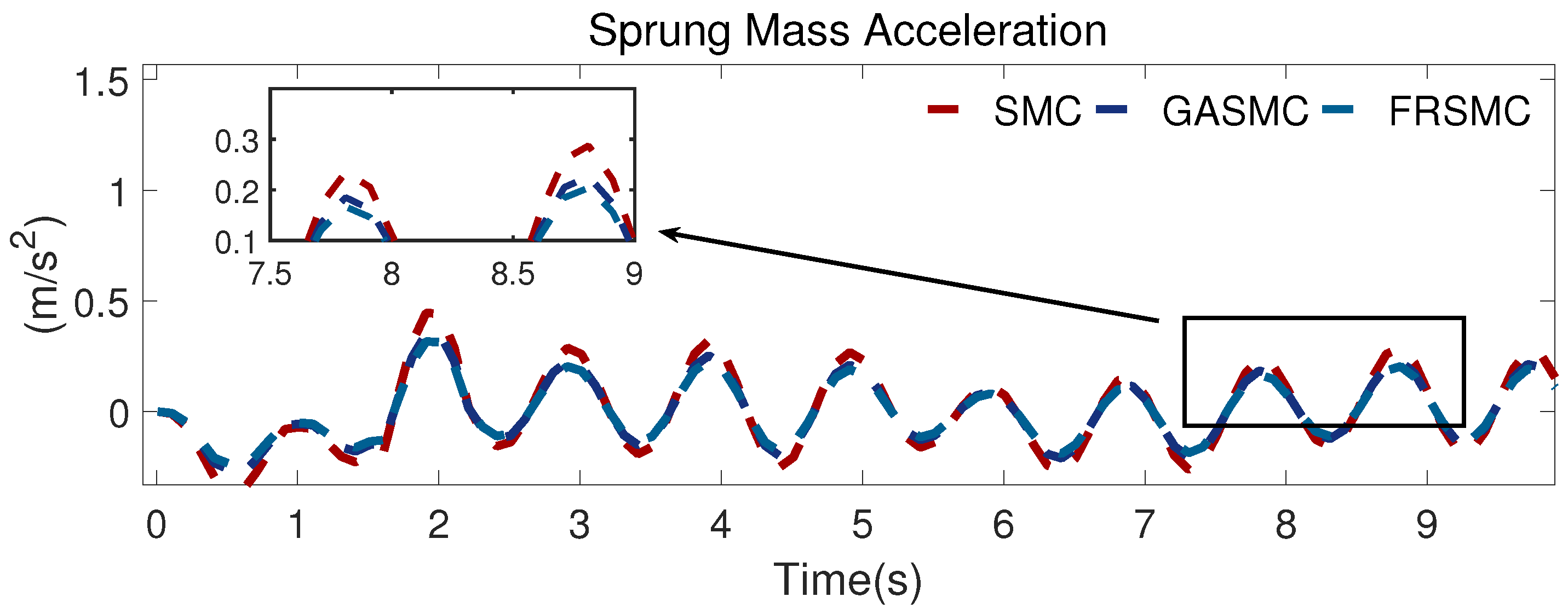
Figure 6 demonstrates the car body mass acceleration for a nonlinear suspension with the SMC, GASMC, and FRSMC control strategies. We find that the proposed controller leads to a smaller car body acceleration than that of the SMC and GASMC strategies, which means that the vertical motion performance is better for ride comfort with the RBF-based fractional-order SMC controller.

Figure 7 displays the pitch angle acceleration obtained when using the SMC, GASMC, and proposed control strategies. We can see in Figure 7 that the pitch angle acceleration can be suppressed to a smaller amplitude with the proposed FRSMC method than it can with the other two control methods; thus, it is implied that the performance of the proposed controller in terms of ride comfort is more superior to that of the SMC and GASMC methods for suspension control.

Figure 8 and Figure 9 show the simulation outcomes for the front and rear suspension deflection. The suspension deflection curves are close to one another in Figure 8 and Figure 9. However, we also find that the suspension deflection curves obtained with the FRSMC are smaller than those of the SMC and GASMC methods. These results show that the driving stability performance with the proposed controller is better than that obtained with the others.

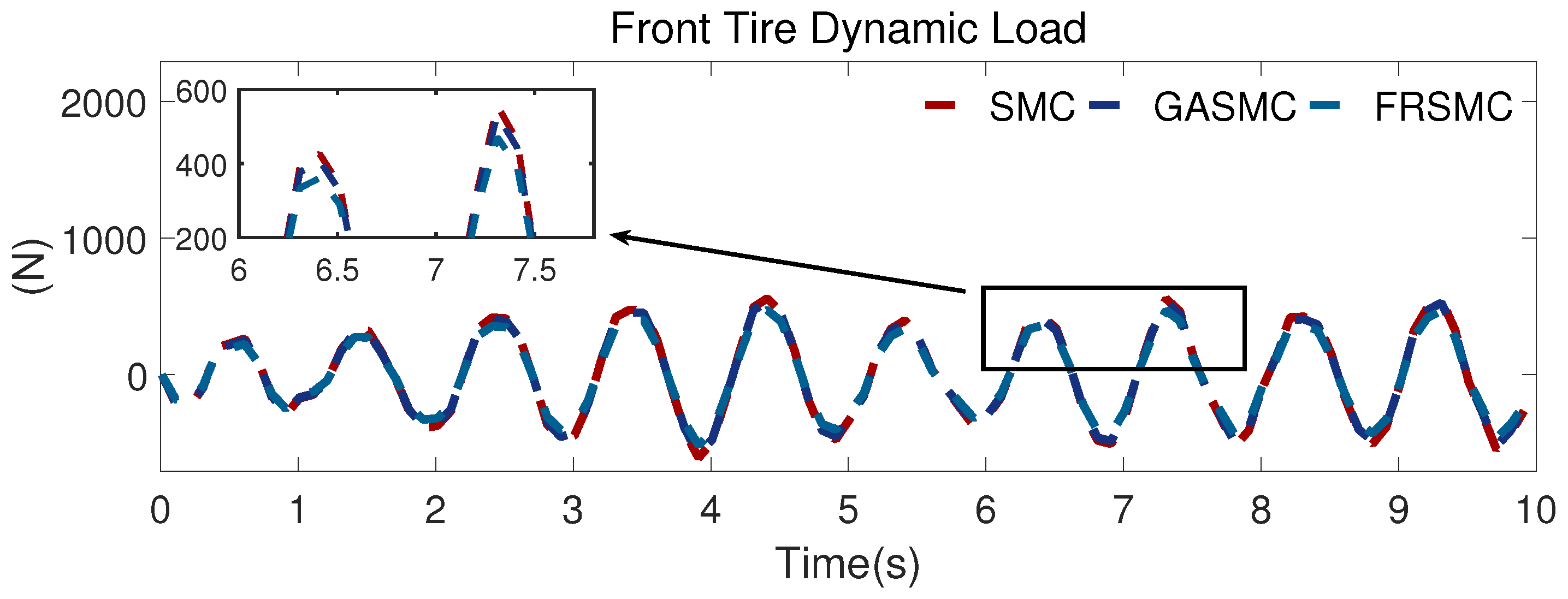
The results for the front- and rear-tire dynamic load are presented in Figure 10 and Figure 11. It is clear that, compared with that obtained with SMC and GASMC, the tire dynamic load curve is smoother with FRSMC. These simulation results also provide evidence that the control performance with the proposed controller is more remarkable.

Table 1 shows the simulation results in terms of the RMS values and depicts a comparison among SMC, GASMC, and FRSMC. We also calculated the percentage by which the performance in terms of ride comfort and handling stability increased in comparison with the single sliding-mode control and genetic algorithm control methods. Figure 12 shows the degree of improvement. As can be seen in Table 1 and Figure 12, compared with that of SMC, the RMS value decreased by 21.12% and 28.99% with GASMC and FRSMC. For the pitch angle acceleration, the RMS value decreased by 5.49% and 16.5% with GASMC and FRSMC in comparison with SMC. With the proposed controller, the front and rear suspension deflection improved by 18.66% and 22.05%, respectively, which is better than the control effect obtained with GASMC. For the tire dynamic load, we also find that the RMS value declines by 15.3% and 16.61%, respectively, in comparison with that of the SMC.

According to the RMS values of the performance indicators, the suspension with the proposed FRSMC provides an obvious improvement, which implies that the suspension capabilities are ameliorated to some extent. The above simulation results show that the proposed RBF-based fractional-order SMC controller performs better than the single SMC and GASMC in the case of no actuator fault.

4.2. Case of Actuator Fault

In the case of actuator fault, which means that actuators cannot work normally, the matrix is $M=\left[\begin{array}{cc}{\delta }_1& 0\\ 0& {\delta }_2\end{array}\right]=\left[\begin{array}{cc}0.5& 0\\ 0& 0.5\end{array}\right]$.

In this section, an extensive simulation is used to demonstrate the effectiveness of the proposed controller. An active suspension with the particle-swarm-optimization-based SMC fault-tolerant control method (PSFTC) and RBF-based fractional-order SMC fault-tolerant control (FRFTC) in the case of actuator fault are used for comparison.

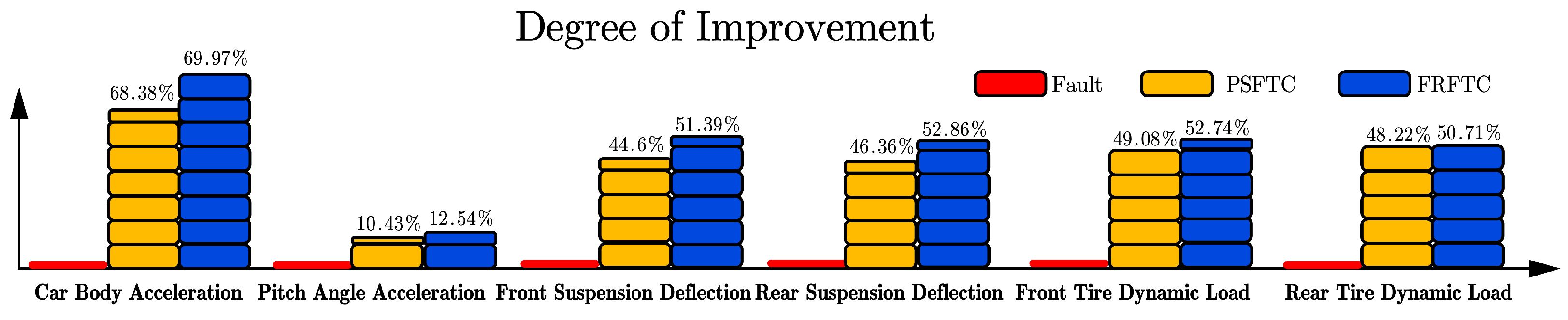
The simulation results in the case of actuator fault are shown in Figure 13, Figure 14, Figure 15, Figure 16, Figure 17 and Figure 18. Figure 19 presents the degree of improvement compared with the fault. The RMS values of the evaluation indicators in the case of no actuator fault are shown in Table 2. In Figure 13, Figure 14, Figure 15, Figure 16, Figure 17, Figure 18 and Figure 19 and Table 2, “$\mathbf{Fault}$” represents the actuator fault in an active suspension, “$\mathbf{PSFTC}$” represents the active suspension with the particle-swarm-optimization-based SMC fault-tolerant controller, and “$\mathbf{FRFTC}$” represents the active suspension with the proposed fault-tolerant controller; that is, the RBF-based fractional-order SMC fault-tolerant controller.

Compared with the actuator fault and fault-tolerant control, it is obvious that the car body acceleration, pitch angle acceleration, suspension deflection, and tire dynamic load fluctuate greatly. It is also obvious that the vibration produced by the road input is much more attenuated when using the fault-tolerant FRFTC.

Figure 13 demonstrates the car body mass acceleration with a nonlinear suspension in the environment of actuator faults with fault-tolerant PSFTC and the designed fault-tolerant controller. It can be seen in Figure 13 that the proposed FRFTC leads to a smaller car body acceleration than that obtained under the fault conditions and with the PSFTC strategy, which means that the vertical motion of the car body provides better ride comfort when using the fault-tolerant FRFTC.

Figure 14 indicates the pitch angle acceleration in the case of actuator fault and with the PSFTC and FRFTC. We can see in Figure 14 that the pitch angle acceleration can be suppressed to a smaller amplitude with the proposed FRFTC method than with the actuator fault; thus, it is implied that the driving stability of the proposed fault-tolerant controller is superior when maintaining the suspension performance when an actuator failure occurs.

Figure 15 and Figure 16 show the front and rear suspension deflection in the simulation outcomes. It can be seen in Figure 15 and Figure 16 that the suspension deflection curves with the FRFTC are smaller than those in the fault case and the PSFTC method. These results show that the driving stability performance with the proposed controller is better than that with the PSFTC, and the controller is able to bring the fault suspension close to the regular state.

The results of the front- and rear-tire dynamic load are shown in Figure 17 and Figure 18. It is clear that, compared with the fault case, both the PSFTC and FRFTC can improve the suspension performance. However, the control effect of the FRFTC is better. These simulation results also provide evidence that the control performance of the proposed fault-tolerant controller is more remarkable.

Table 3 shows the simulation results in terms of the RMS values in a comparison among faults, the PSFTC, and the FRFTC. Figure 19 shows the degree of improvement. As can be seen in Table 3 and Figure 19, it is easily noted that, compared with the actuator fault case, the RMS values decreased by 68.38% and 69.97% with the GASMC and FRSMC. For the pitch angle acceleration, the RMS values decreased by 10.43% and 12.54% with the PSFTC and FRFTC in comparison with the fault case. With the proposed controller, the front and rear suspension deflection improved by 51.39% and 52.86%, respectively, which is better than the control effect with the PSFTC. For the tire dynamic load, we also find that the RMS values declined by 52.74% and 50.71%, respectively, compared with those in the fault case.

5. Discussion and Conclusions

The problem of the fault-tolerant control of actuators was addressed by using a half-car model. An RBF-based fractional-order SMC controller (FRSMC controller) was proposed to enhance vehicles’ dynamic performance in the presence of faults. The proposed hybrid control strategy was exploited to improve the control by accounting for actuator failure. The proposed control law was designed to ensure comfort and stability in suspension system performance on the road.

To overcome the jitter vibration problem in SMC, fractional-order theory and RBF neural networks were used in the proposed controller, and an RBF neural network was also used to obtain the optimal switching gain.

To verify the effectiveness of the proposed control method, two cases consisting of no actuator fault and actuator fault were presented. In the case of no actuator fault, a genetic-algorithm-based sliding-mode controller was compared with the proposed control method. In the case of actuator fault, a particle-swarm-optimization-based sliding-mode control was applied to make a comparison with the proposed method.

According to the simulation results, it was confirmed that the RBF-neural-network-based fractional-order sliding-mode controller had good convergence and control effects. In the case of no actuator fault, the SMC method and genetic-algorithm-based SMC were compared with the proposed control method in healthy cases. Ultimately, addressing these comparisons, it is clear that the controller discussed in this study has better control effects. This confirms the performance of the proposed control algorithm. In the case of actuator fault, the actuator fault problem was considered. A PSO-based SMC fault-tolerant controller and the proposed controller under fault conditions were compared. As shown by the comparison, the fault control method proposed in this study performed better than the other method under the conditions of suspension fault. Therefore, in the case of failure, with the controller proposed in this study, the state of the suspension is essentially the same as that of a healthy suspension. According to the simulation results, this dependable controller can guarantee improved suspension performance in the presence of no actuator faults and the case of such faults.

However, suspension systems are large and complex, and the fault models examined in this study are assumed. This type of failure does not exist in practice. Actual faults come in many forms, and they do not include only gain faults. Faults are also randomized, as is the size of the gain.

Our future research will focus on the following main areas: the suggested control strategy will be implemented in a vehicle system, the nonlinear model will be made more accurate, and a full-automobile dynamic model will be created by using the FRFTC in a real car.

References

- Jin, P.; Xue, W.; Li, K. Actuator Fault Estimation for Vehicle Active Suspensions Based on Adaptive Observer and Genetic Algorithm. Shock Vib. 2019, 3, 1783850. [Google Scholar] [CrossRef]
- Du, H.; Yim, S.K.; Lam, J. Semi-active H∞ control of vehicle suspension with magneto-rheological dampers. J. Sound Vib. 2005, 283, 981–996. [Google Scholar] [CrossRef]
- Shao, X.; Naghdy, F.; Du, H. Reliable fuzzy H-infinity control for active suspension of in-wheel motor driven electric vehicles with dynamic damping. Mech. Syst. Signal Process. 2017, 87, 365–383. [Google Scholar] [CrossRef]
- Chen, L.; Wang, S.; Sun, X.; Yuan, C.; Cai, Y. Model predictive control of an air suspension system with a damping multi-mode switching damper based on a hybrid model. Mech. Syst. Signal Process. 2017, 94, 94–110. [Google Scholar]
- Chen, H.; Guo, K.H. Constrained H∞ control of active suspensions: An LMI approach. IEEE Trans. Control. Syst. Technol. 2005, 13, 412–421. [Google Scholar] [CrossRef]
- Zhang, L.P.; Gong, D.L. Passive fault-tolerant control for vehicle active suspension system based on H2/H∞ approach. J. Vibroeng. 2018, 20, 1828–1849. [Google Scholar] [CrossRef]
- Hu, Y.; Hou, Z. Multiplexed model predictive control for active vehicle suspensions. Int. J. Control 2014, 88, 347–363. [Google Scholar] [CrossRef]
- Liang, J.; Lu, Y.; Pi, D. A decentralized cooperative control framework for active steering and active suspension: Multi-agent approach. IEEE Trans. Transp. Electrif. 2022, 8, 1414–1429. [Google Scholar] [CrossRef]
- Wang, Z.; Unbehauen, H. Robust Hinfinity Control for Systems with Time-Varying Parameter Uncertainty and Variance Constraints. Cybern. Syst. 2000, 31, 175–191. [Google Scholar]
- Kim, C.; Ro, P.I. A sliding mode controller for vehicle active suspension systems with non-linearities. Proc. Inst. Mech. Eng. Part D J. Automob. Eng. 2016, 212, 79–92. [Google Scholar] [CrossRef]
- Yang, G.; Zhang, S. Reliable Control Using Redundant Controllers. IEEE Trans. Autom. Control 1998, 43, 1588. [Google Scholar] [CrossRef]
- Peng, S.; El Kebir, B.; Sing, K.N.; Guo, X. Robust disturbance attenuation for discrete-time active fault tolerant control systems with uncertainties. Optim. Control. Appl. Methods 2003, 24, 85–101. [Google Scholar]
- Chamseddine, A.; Noura, H. Control and Sensor Fault Tolerance of Vehicle Active Suspension. IEEE Trans. Control. Syst. Technol. 2008, 16, 416–433. [Google Scholar] [CrossRef]
- Li, H.; Liu, H.; Gao, H.; Shi, P. Reliable Fuzzy Control for Active Suspension Systems With Actuator Delay and Fault. IEEE Trans. Fuzzy Syst. 2012, 20, 342–357. [Google Scholar] [CrossRef]
- Wang, R.; Jing, H.; Karimi, H.R.; Chen, N. Robust fault-tolerant H∞ control of active suspension systems with finite-frequency constraint-ScienceDirect. Mech. Syst. Signal Process. 2015, 62–63, 341–355. [Google Scholar] [CrossRef]
- Feng, C.; Hao, S.; Li, Y.; Tong, S. Fuzzy Adaptive Fault-Tolerant Control for a Class of Active Suspension Systems with Time Delay. Int. J. Fuzzy Syst. 2019, 21, 2054–2065. [Google Scholar]
- Soon, K.B.; Daejun, K.; Kyongsu, Y. Fault-tolerant control with state and disturbance observers for vehicle active suspension systems. Proc. Inst. Mech. Eng. Part D J. Automob. Eng. 2020, 234, 1912–1929. [Google Scholar]
- Utkin Vadim, I.; Chang, H.C. Sliding mode control on electro-mechanical systems. Math. Probl. Eng. 2002, 8, 451–473. [Google Scholar] [CrossRef]
- Morteza, M.; Afef, F. Adaptive PID-Sliding-Mode Fault-Tolerant Control Approach for Vehicle Suspension Systems Subject to Actuator Faults. IEEE Trans. Veh. Technol. 2014, 63, 1041–1054. [Google Scholar]
- Li, M.; Zhang, Y.; Geng, Y. Fault-tolerant sliding mode control for uncertain active suspension systems against simultaneous actuator and sensor faults via a novel sliding mode observer. Optim. Control. Appl. Methods 2018, 39, 1728–1749. [Google Scholar] [CrossRef]
- Slotine, J.J.E. Tracking Control of Nonlinear System Using Sliding Surface with Application to Robot Manipulator. Int. J. Control 1983, 38, 465–492. [Google Scholar] [CrossRef]
- Slotine, J.J.E. Sliding Controller Design for Non-linear Systems. Int. J. Control 1984, 40, 421–434. [Google Scholar] [CrossRef]
- Gao, W.; Hung, J.C. Variable Structure Control of Nonlinear Systems: A New Approach. IEEE Trans. Ind. Electron. 1993, 40, 45–55. [Google Scholar]
- Zou, X.; Ding, H.; Li, J. Sensorless Control Strategy of Permanent Magnet Synchronous Motor Based on Fuzzy Sliding Mode Controller and Fuzzy Sliding Mode Observer. J. Electr. Eng. Technol. 2023, 18, 2355–2369. [Google Scholar] [CrossRef]
- Ming, Y.; Cong, S.; Xu, J. Design of Nonlinear Motor Adaptive Fuzzy Sliding Mode Controller Based on GA. J. Syst. Simul. 2008, 20, 3141–3145. [Google Scholar]
- Zhang, Q.; Zhang, Q.; Jiang, C.; Huang, H.; Zhang, S. Research on SMC Control of Permanent Magnet Synchronous Motor System Based on Particle Swarm Optimization. Equip. Manuf. Technol. 2019, 4, 35–39. [Google Scholar]
- Guo, X.; Liu, X. Particle swarm optimization sliding mode control on interconnected power system. In Proceedings of the 33rd Chinese Control Conference, Nanjing, China, 28–30 July 2014. [Google Scholar]
- Saleh, T.M.; Mohammad, H. Synchronization of chaotic fractional-order systems via active sliding mode controller. Phys. Stat. Mech. Its Appl. 2008, 387, 57–70. [Google Scholar]
- Zhang, Y. Time domain model of road irregularities simulated using the harmony superposition method. Trans. Chin. Soc. Agric. Eng. 2003, 19, 32–35. [Google Scholar]
- Liu, X.; Pang, H.; Shang, Y. An Observer-Based Active Fault Tolerant Controller for Vehicle Suspension System. Appl. Sci. 2018, 8, 2568. [Google Scholar] [CrossRef]
- Chen, W.; Zhao, L. Intelligent Vehicle Fault Tolerant Control Technology and Application; Science Press: Beijing, China, 2021. [Google Scholar]
- Podlubny, I. Fractional Differential Equations. In Mathematics in Science and Engineering; Academic Press: San Diego, CA, USA, 1999. [Google Scholar]
- Li, H.; Yu, J.; Hilton, C. Adaptive Sliding-Mode Control for Nonlinear Active Suspension Vehicle Systems Using T–S Fuzzy Approach. IEEE Trans. Ind. Electron. 2013, 60, 3328–3338. [Google Scholar] [CrossRef]
- Duarte-Mermoud, M.; Aguila-Camacho, N. Using general quadratic Lyapunov functions to prove Lyapunov uniform stability for fractional order systems. Commun. Nonlinear Sci. Numer. Simul. 2015, 22, 650–659. [Google Scholar] [CrossRef]
Figure 1.
Front road input.
Figure 2.
Rear road input.
Figure 3.
Half-car suspension model.
Figure 4.
Schematic of the RBF structure.
Figure 5.
Schematic of the controller structure.
Figure 6.
Sprung mass acceleration.
Figure 7.
Pitch angle acceleration.
Figure 8.
Front suspension deflection.
Figure 9.
Rear suspension deflection.
Figure 10.
Front-tire dynamic deflection.
Figure 11.
Rear-tire dynamic deflection.
Figure 12.
Degree of improvement.
Figure 13.
Figure 14.
Figure 15.
Figure 16.
Figure 17.
Figure 18.
Figure 19.