
Study on the Kinematic Performances and Optimization for Three Types of Parallel Manipulators

Abstract
:1. Introduction
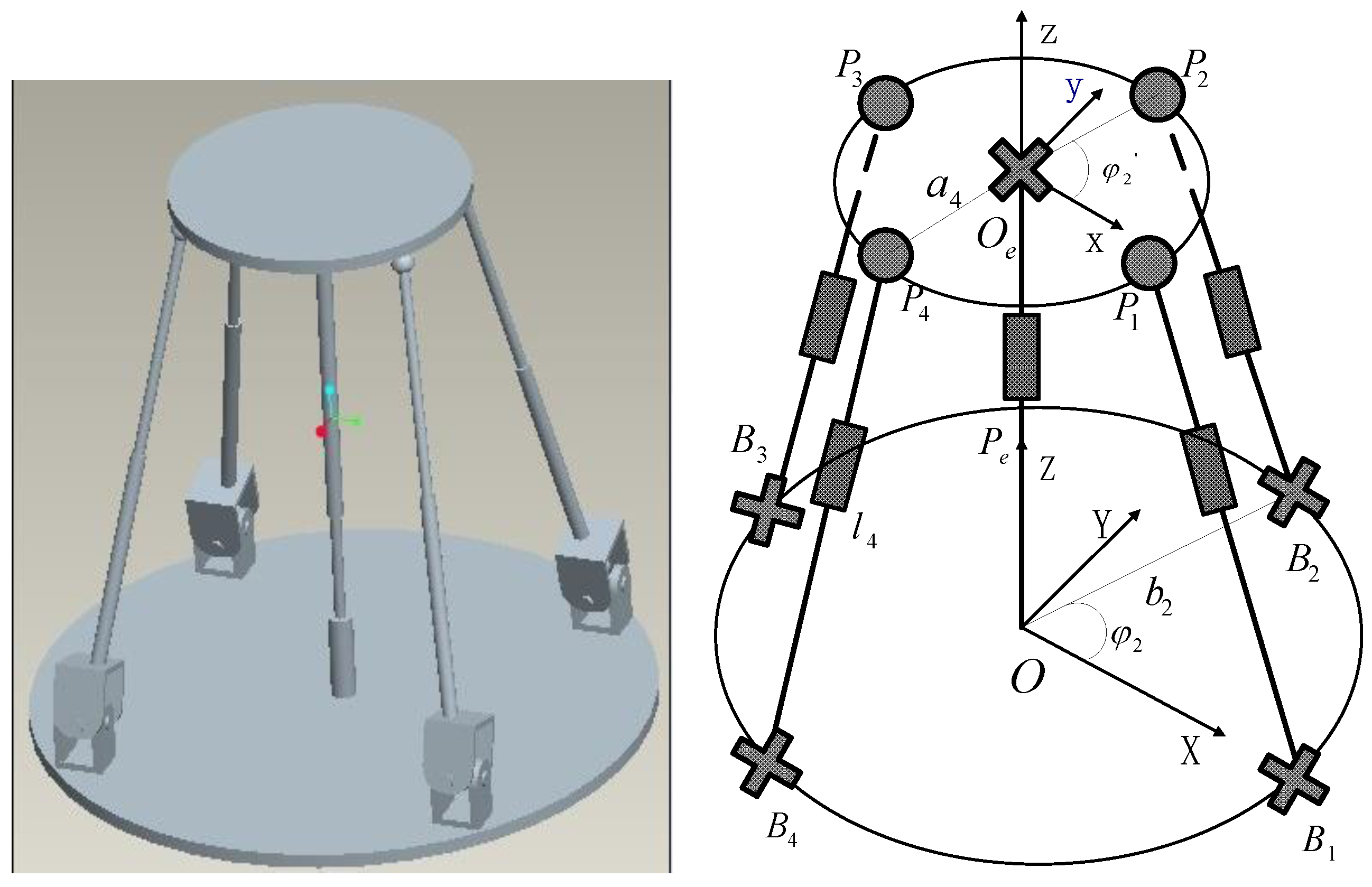
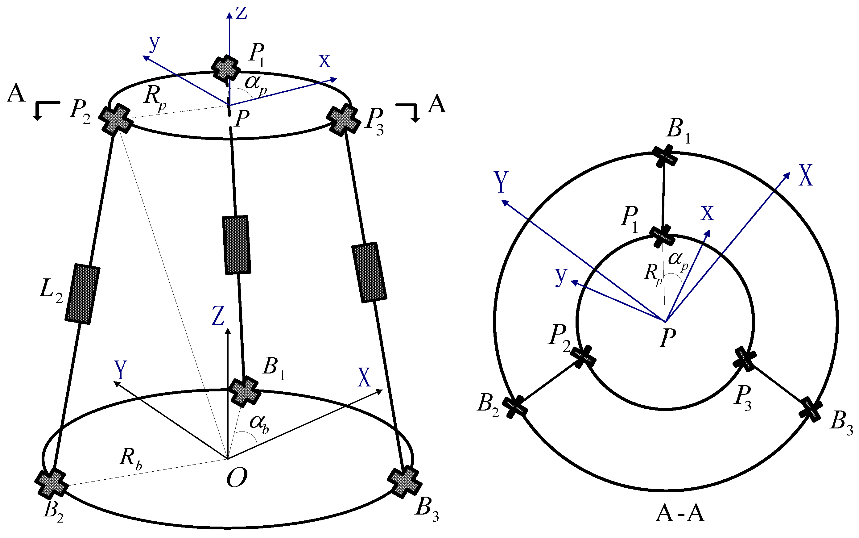
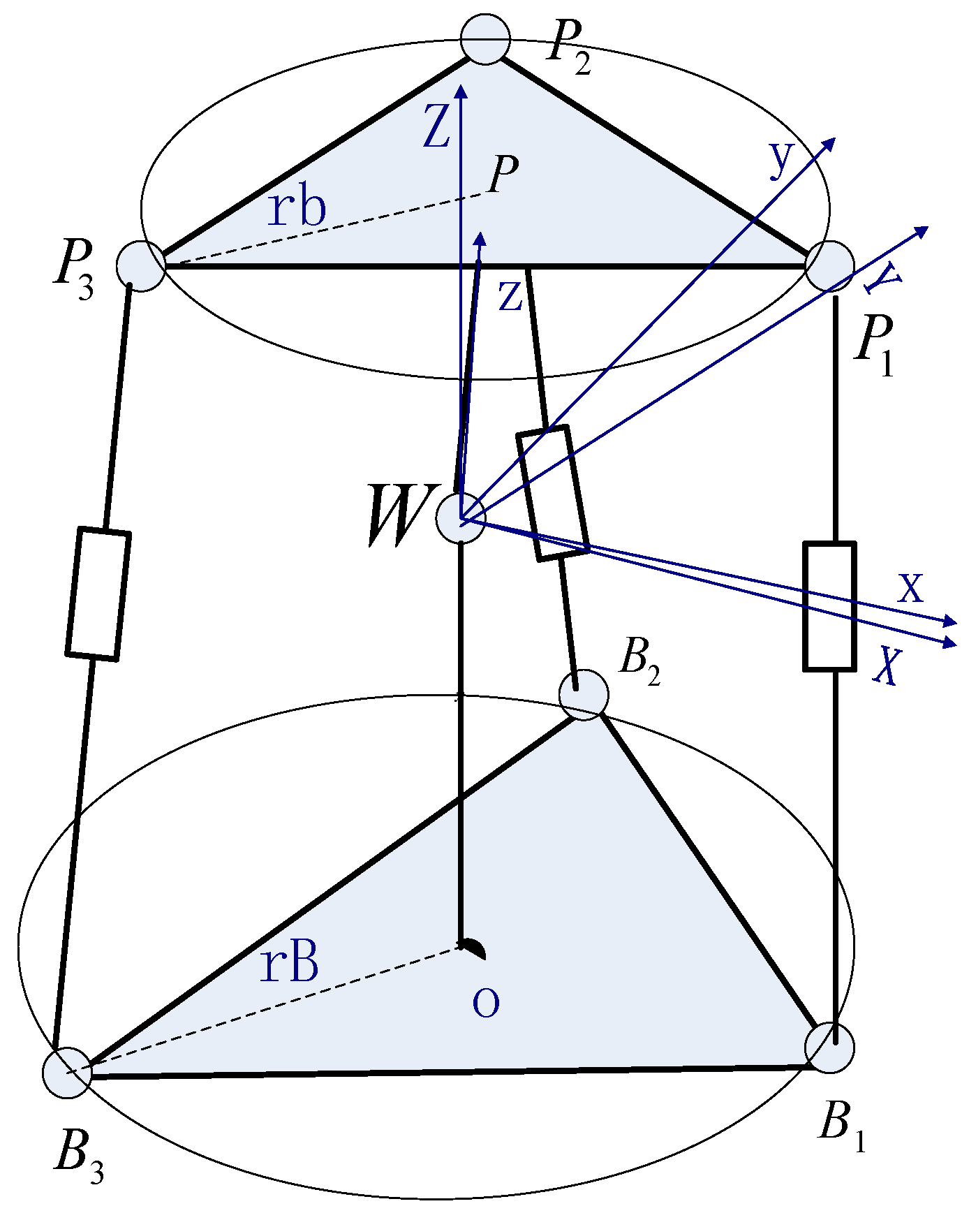
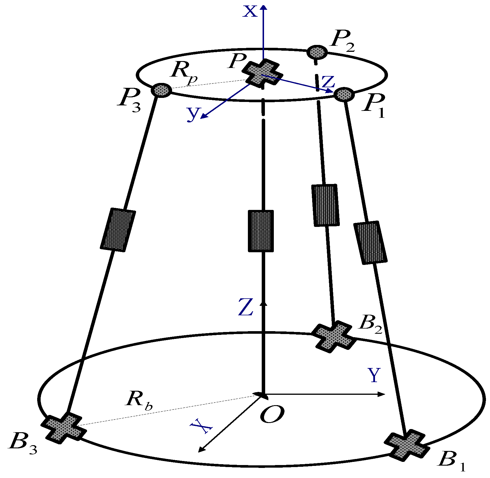
2. Kinematic Analysis and Modelling
2.1. Pure Translational Case
2.2. Pure Rotational Case
2.3. Mixed Motion Case
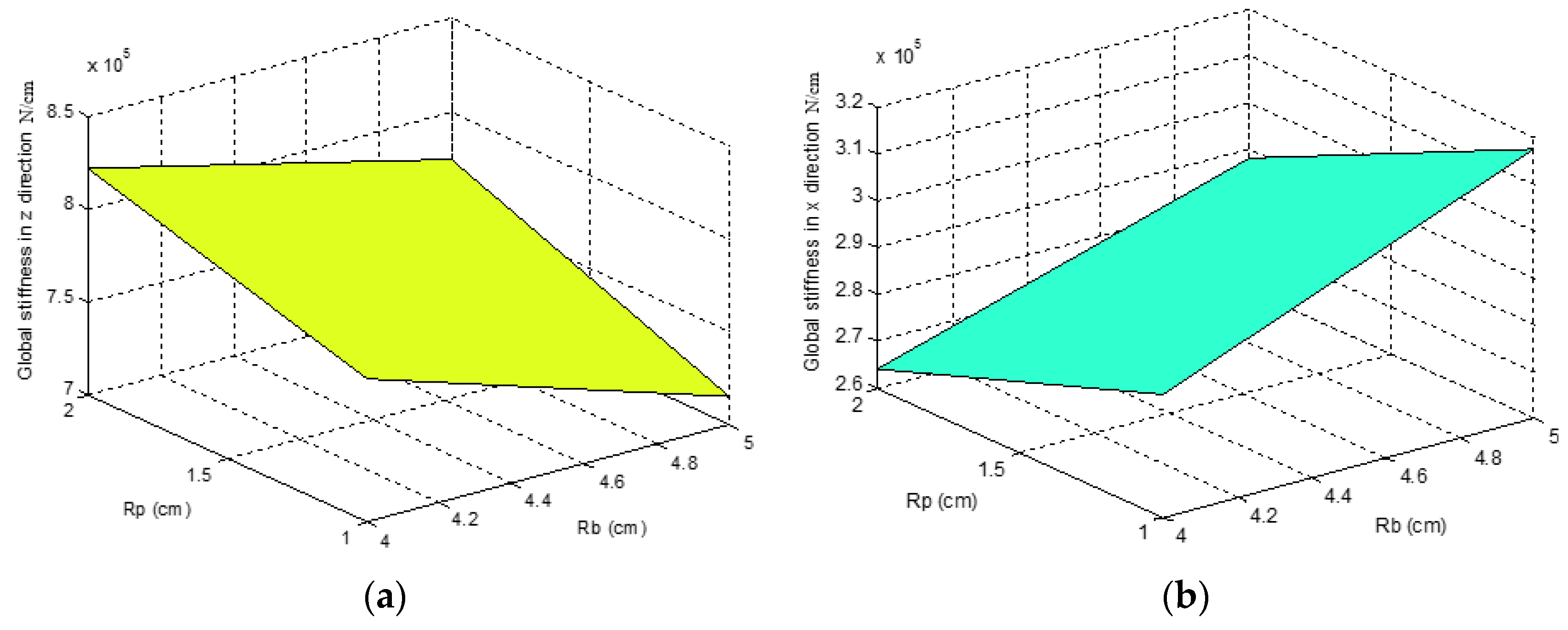
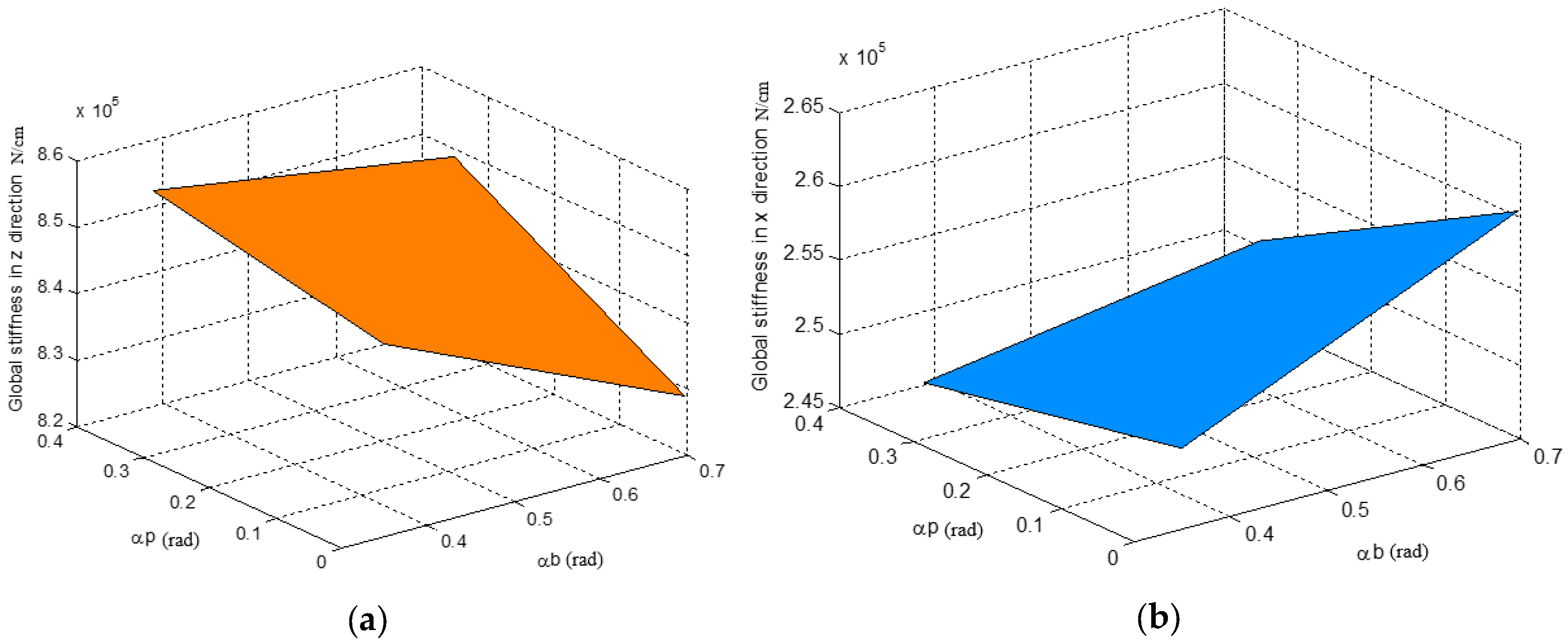
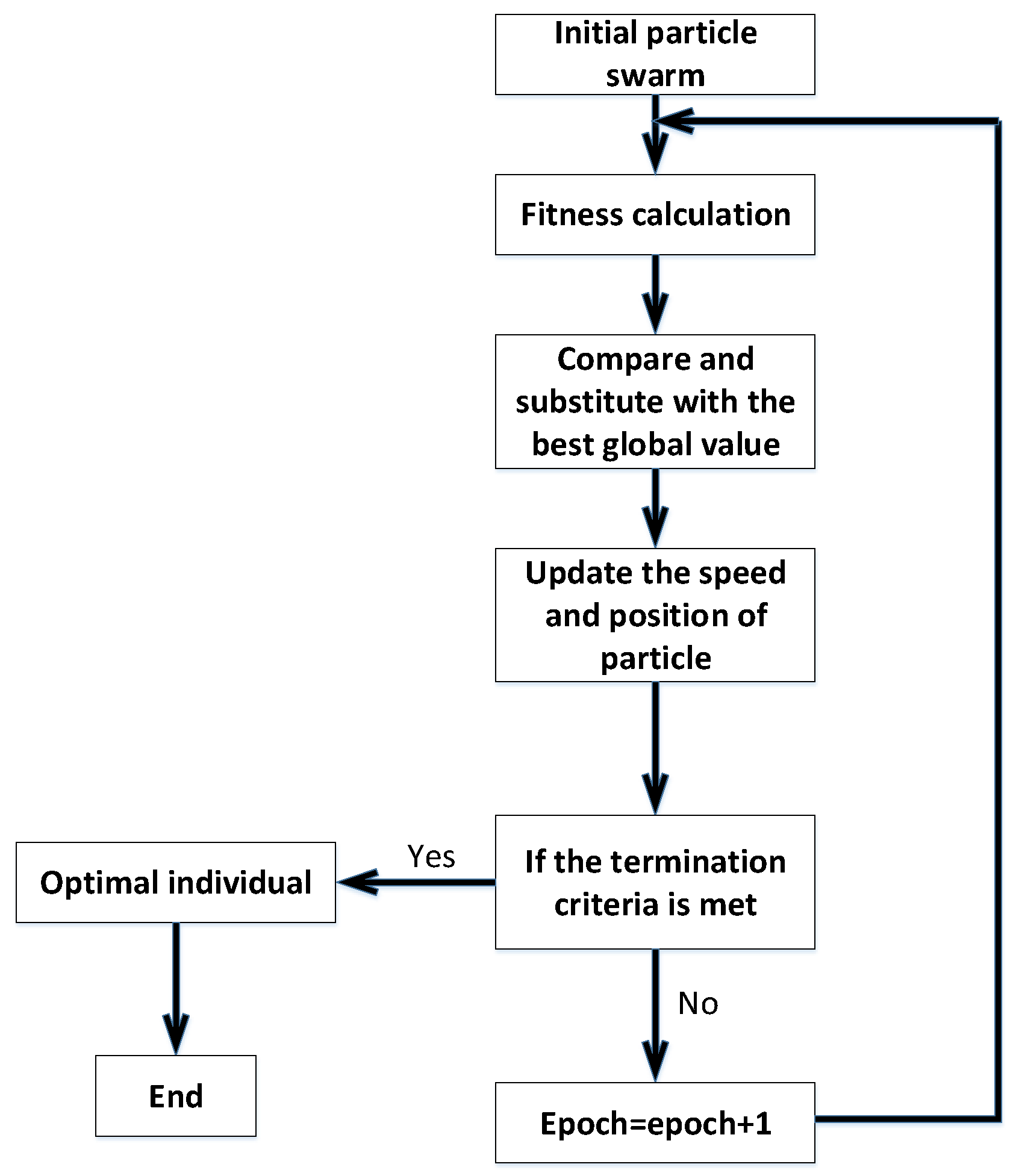
3. Optimization Discussion and Modelling
3.1. Pure Translational Case
3.2. Pure Rotational Case
3.3. Mixed Motion Case
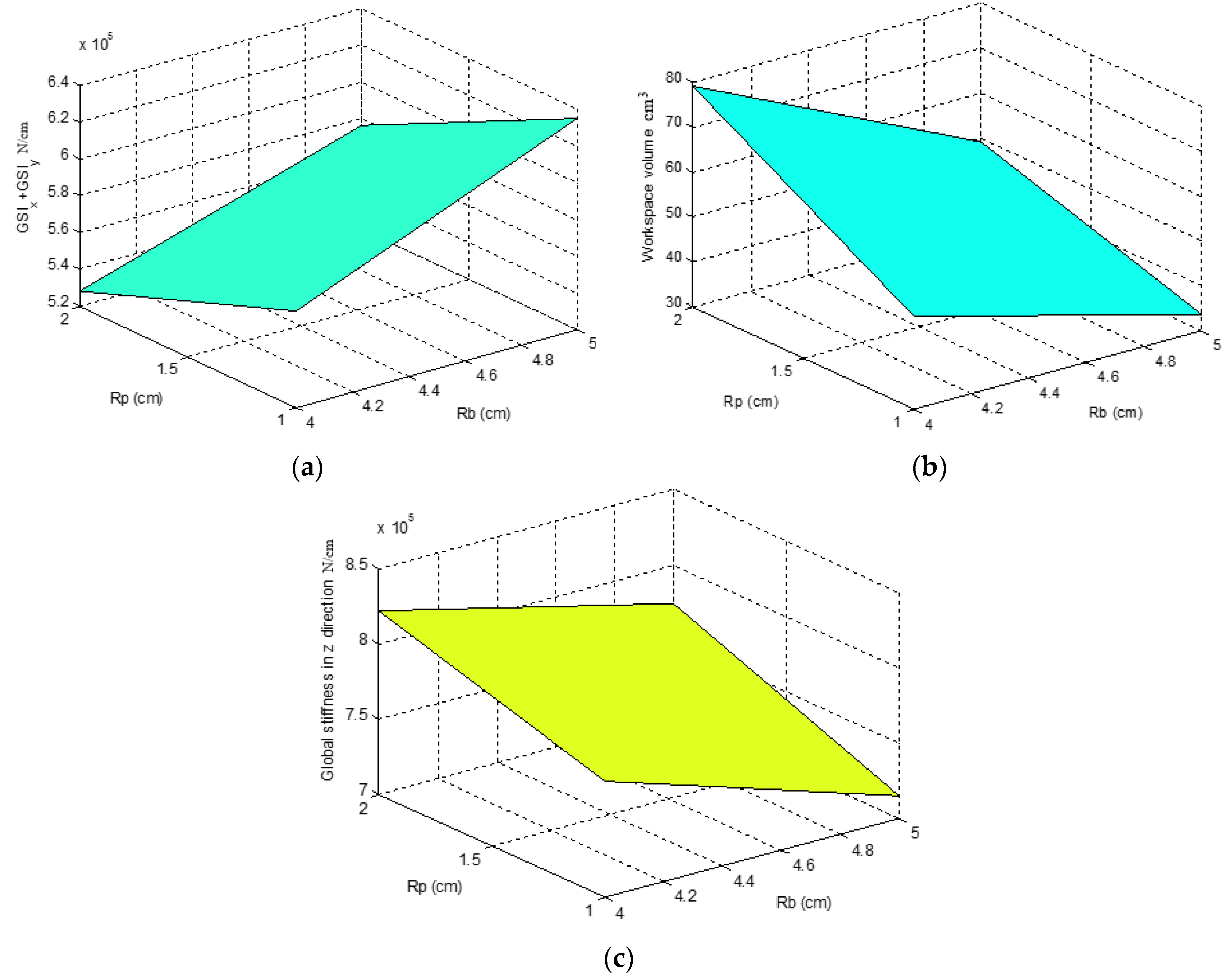
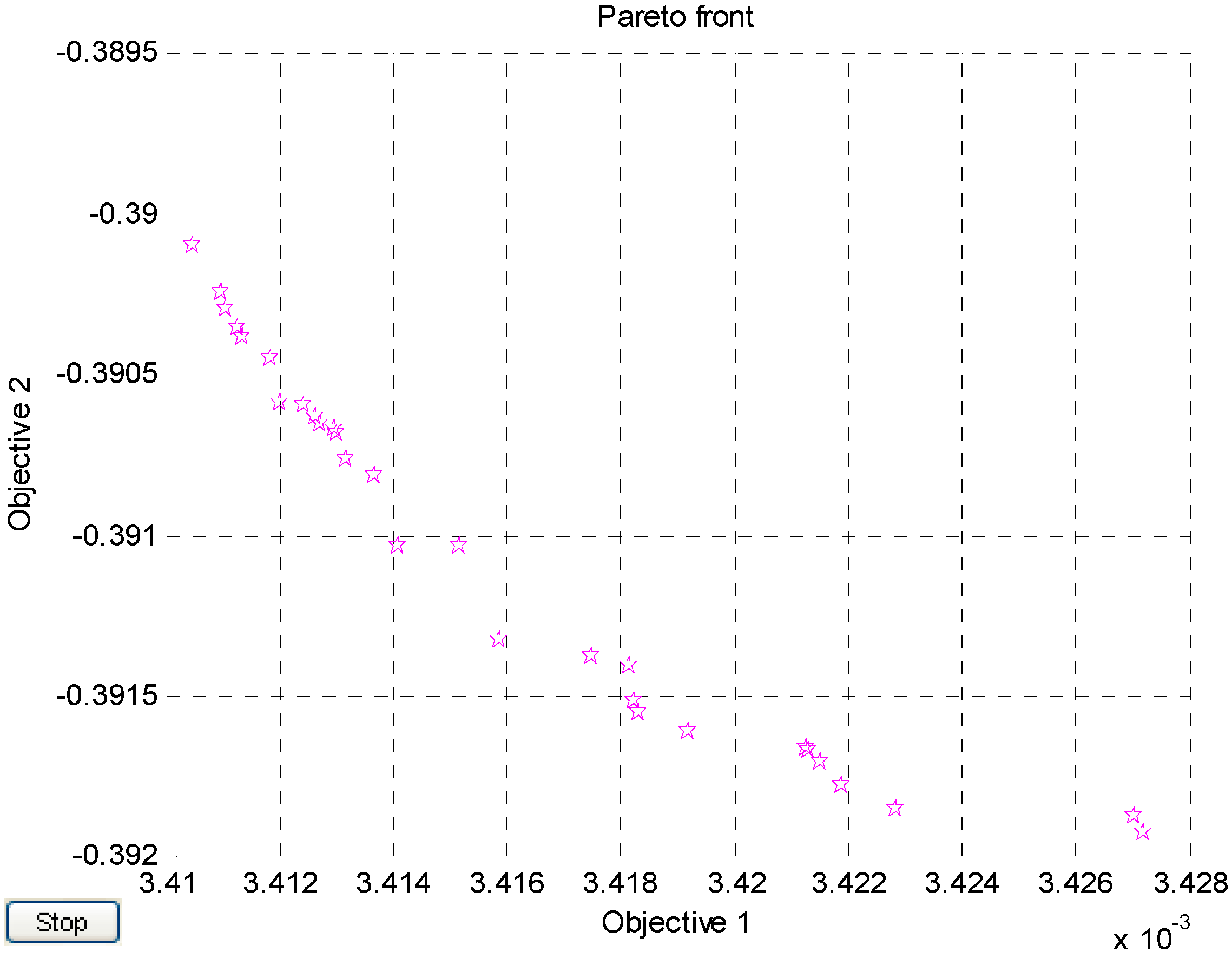
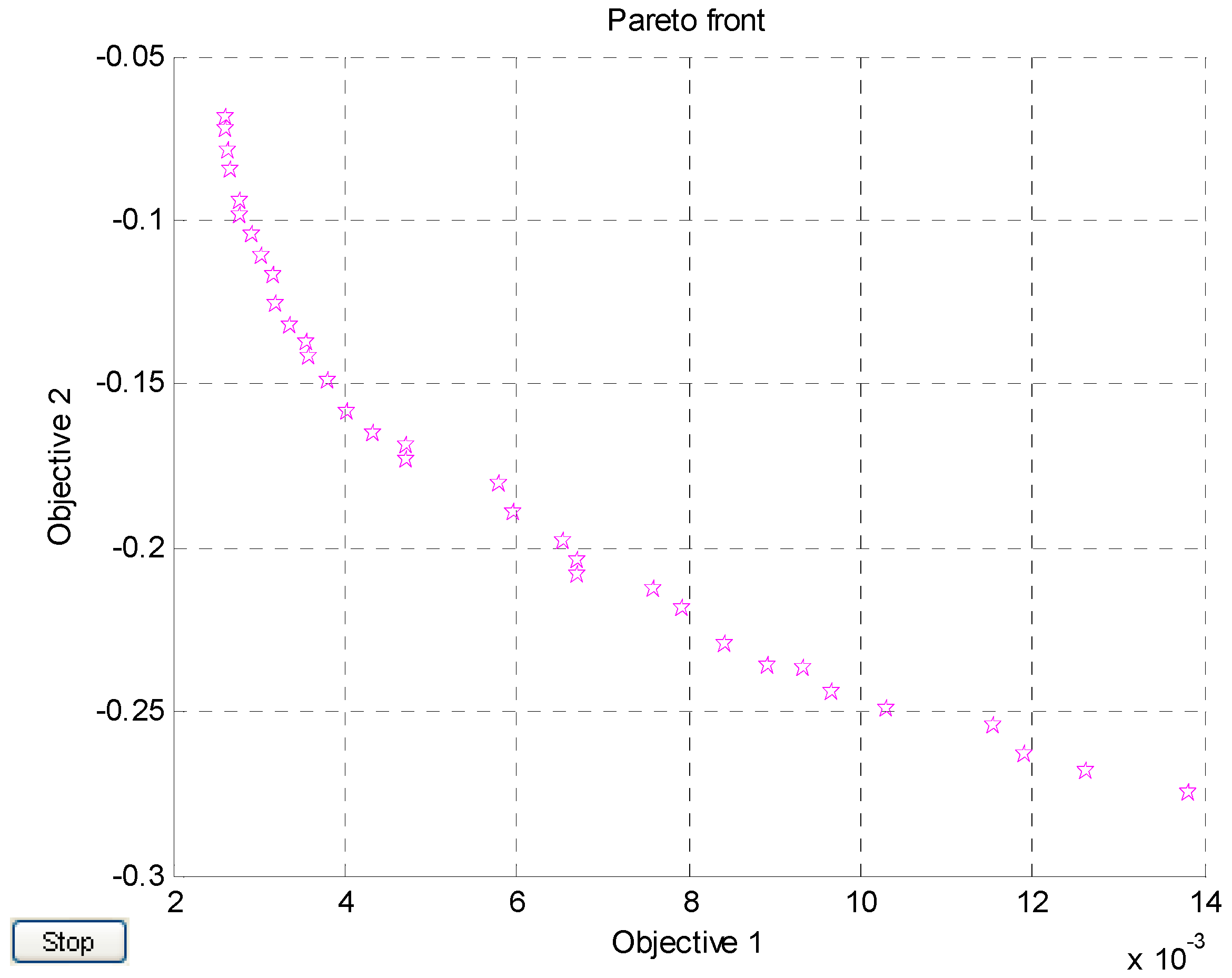
4. Optimization Results
4.1. Pure Translational Case
4.2. Pure Rotational Case
4.3. Mixed Motion Case
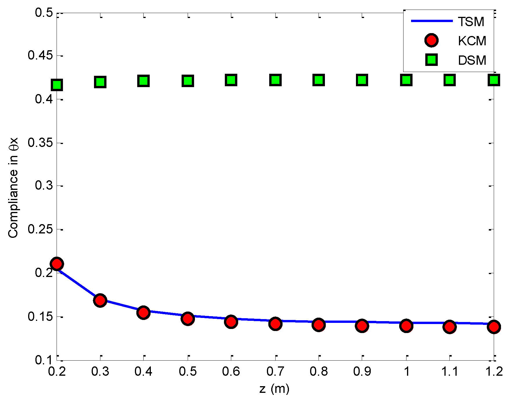
5. Stiffness Models
5.1. TSM Case
5.2. KCM Case
5.3 DSM Case
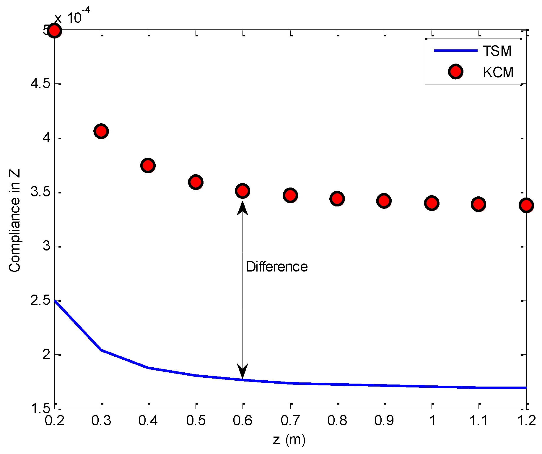
6. Comparisons
6.1. Three Cases
6.2. Comparison
7. Conclusions
Acknowledgments
Author Contributions
Conflicts of Interest
References
- Li, Y.; Xu, Q. Design and Development of a Medical Parallel Robot for Cardiopulmonary Resuscitation. IEEE/ASME Trans. Mechatron. 2007, 12, 265–273. [Google Scholar] [CrossRef]
- Sakai, S.; Lida, M.; Umeda, M. Heavy material handling manipulator for agricultural robot. In Proceedings of the IEEE International Conference on Robotics and Automation, Washington, DC, USA, 11–15 May 2002; pp. 1062–1068.
- Sakai, S.; Osuka, K.; Maekawa, T.; Umeda, M. Robust Control Systems of a Heavy Material Handling Agricultural Robot: A Case Study for Initial Cost Problem. IEEE Trans. Control Syst. Technol. 2007, 15, 1038–1048. [Google Scholar] [CrossRef]
- Zhang, D.; Wei, B. Design and analysis of a collision detector for hybrid robotic machine tools. Sens. Transducers J. 2015, 193, 67–73. [Google Scholar]
- Bohez, E. Five-axis milling machine tool kinematic chain design and analysis. Int. J. Mach. Tools Manuf. 2002, 42, 505–520. [Google Scholar] [CrossRef]
- Zhang, D.; Wei, B. Payload variation compensation for robotic arms through model reference control approach. Int. J. Robot. Autom. 2016. [Google Scholar] [CrossRef]
- Liang, Q.; Wu, W.; Zhang, D.; Wei, B. Design and analysis of a micromechanical three-component force sensor for characterizing and quantifying surface roughness. Meas. Sci. Rev. 2015, 15, 248–255. [Google Scholar] [CrossRef]
- Howe, R. Tactile Sensing and Control of Robotic Manipulation. J. Adv. Robot. 1994, 8, 245–261. [Google Scholar] [CrossRef]
- Gosselin, C.; Jorge, A. A Global Performance Index for the Kinematic Optimization of Robotic Manipulators. J. Mech. Des. 1991, 113, 220–226. [Google Scholar] [CrossRef]
- Li, B.; Zhi, W.; Ying, H. The Stiffness Calculation Model of the New Typed Parallel Machine Tool. Mach. Des. 1999, 3, 14–16. [Google Scholar]
- Merlet, J.P. Determination of the Orientation Workspace of Parallel Manipulators. J. Intell. Robot. Syst. 1995, 13, 143–160. [Google Scholar] [CrossRef]
- Stamper, R.E.; Tsai, L.; Walsh, G.C. Optimization of a Three DOF Translational Platform for Well-conditioned Workspace. In Proceedings of the IEEE International Conference on Robotics and Automation, Albuquerque, NM, USA, 25 April 1997; pp. 3250–3255.
- Caponetto, R.; Fortuna, L.; Fazzino, S.; Xibilia, M. Chaotic Sequences to Improve the Performance of Evolutionary Algorithms. IEEE Trans. Evolut. Comput. 2003, 7, 289–304. [Google Scholar] [CrossRef]
- Zhang, D. Parallel Robotic Machine Tools; Springer: New York, NY, USA, 2009. [Google Scholar]
- Zhang, D.; Gao, Z. Forward kinematics, performance analysis, and multi-objective optimization of a bio-inspired parallel manipulator. Robot. Comput.-Integr. Manuf. 2012, 28, 484–492. [Google Scholar] [CrossRef]


| Options | Parameters |
|---|---|
| The size of the population | 50 |
| Maximum of generations | 66 |
| Selection strategy | Tournament |
| The size of tournament | 2 |
| Crossover type | Intermediate |
| Crossover ratio | 1 |
| Pareto front population fraction | 0.7 |
| KCM | TSM | DSM | |
|---|---|---|---|
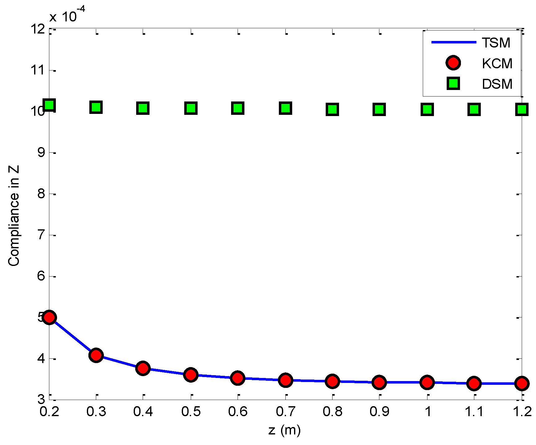
| Z Compliance | 0.0003 | 0.0003 | 0.0010 |
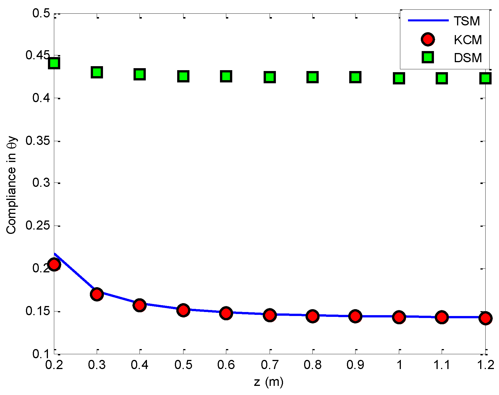
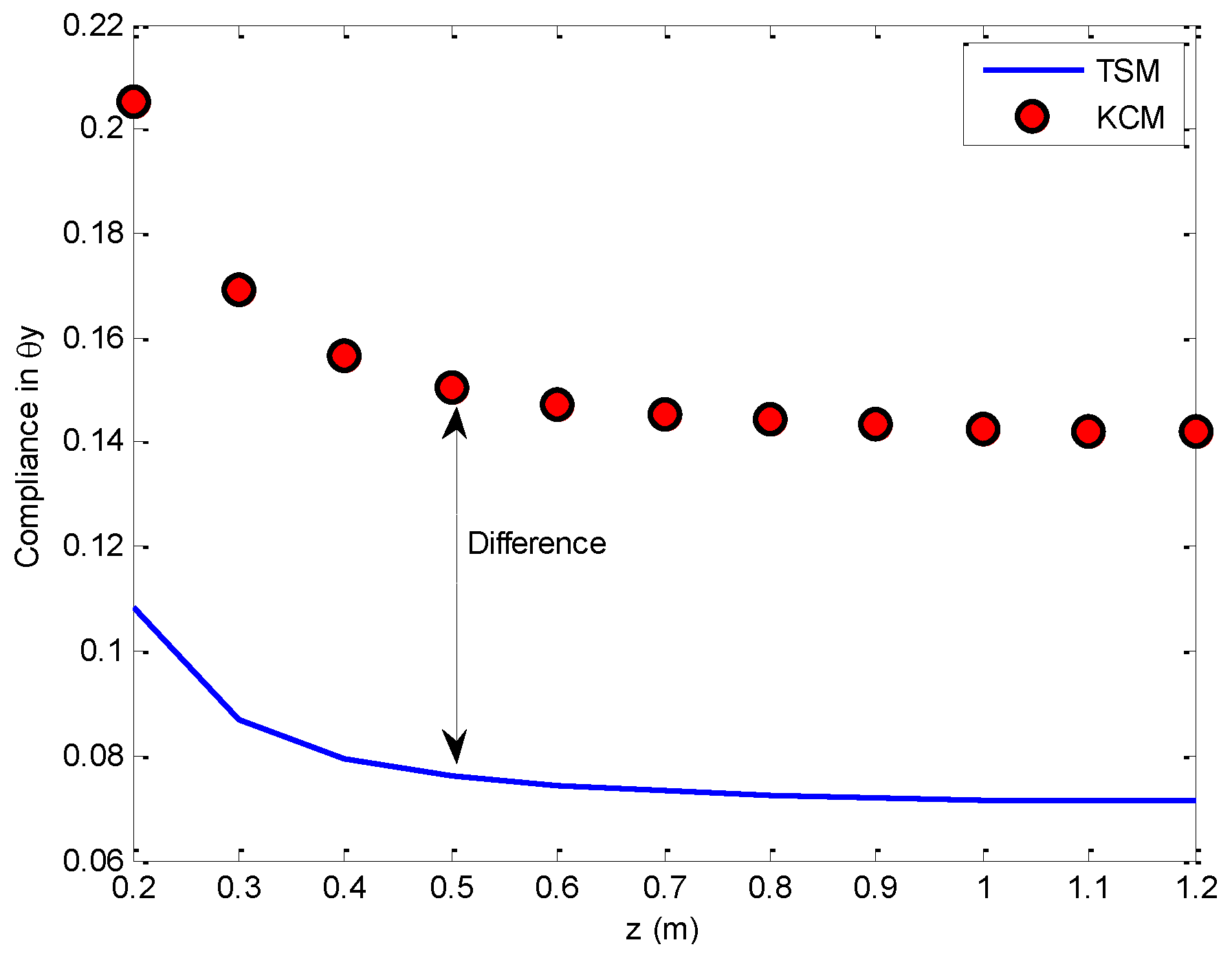
| Compliance | 0.1428 | 0.1461 | 0.4218 |
| Compliance | 0.1461 | 0.1472 | 0.4249 |
| Sum of compliances | 0.2936 | 0.2936 | 0.8477 |
© 2016 by the authors; licensee MDPI, Basel, Switzerland. This article is an open access article distributed under the terms and conditions of the Creative Commons Attribution (CC-BY) license (http://creativecommons.org/licenses/by/4.0/).
Share and Cite
Zhang, D.; Wei, B. Study on the Kinematic Performances and Optimization for Three Types of Parallel Manipulators. Machines 2016, 4, 24. https://doi.org/10.3390/machines4040024
Zhang D, Wei B. Study on the Kinematic Performances and Optimization for Three Types of Parallel Manipulators. Machines. 2016; 4(4):24. https://doi.org/10.3390/machines4040024
Chicago/Turabian StyleZhang, Dan, and Bin Wei. 2016. "Study on the Kinematic Performances and Optimization for Three Types of Parallel Manipulators" Machines 4, no. 4: 24. https://doi.org/10.3390/machines4040024