Experimental Evidence of the Speed Variation Effect on SVM Accuracy for Diagnostics of Ball Bearings


Department of Sciences and Methods of Engineering, University of Modena and Reggio Emilia, Via Amendola 2-Pad. Morselli, 42122 Reggio Emilia, Italy
*
Author to whom correspondence should be addressed.
Machines 2018, 6(4), 48; https://doi.org/10.3390/machines6040048
Submission received: 15 September 2018
/
Revised: 15 October 2018
/
Accepted: 17 October 2018
/
Published: 18 October 2018
(This article belongs to the Special Issue Fault Detection, Diagnosis, and Recovery: Concept, Modeling, and Optimization)
Abstract
:In recent years, we have witnessed a considerable increase in scientific papers concerning the condition monitoring of mechanical components by means of machine learning. These techniques are oriented towards the diagnostics of mechanical components. In the same years, the interest of the scientific community in machine diagnostics has moved to the condition monitoring of machinery in non-stationary conditions (i.e., machines working with variable speed profiles or variable loads). Non-stationarity implies more complex signal processing techniques, and a natural consequence is the use of machine learning techniques for data analysis in non-stationary applications. Several papers have studied the machine learning system, but they focus on specific machine learning systems and the selection of the best input array. No paper has considered the dynamics of the system, that is, the influence of how much the speed profile changes during the training and testing steps of a machine learning technique. The aim of this paper is to show the importance of considering the dynamic conditions, taking the condition monitoring of ball bearings in variable speed applications as an example. A commercial support vector machine tool is used, tuning it in constant speed applications and testing it in variable speed conditions. The results show critical issues of machine learning techniques in non-stationary conditions.
1. Introduction
The monitoring of rotating and translating machines [1] cannot be separated from the surveillance of the health from the supports. This is why rolling bearings have always been the primary object of study for the diagnosis of malfunctions in mechanical systems, with the aim of ensuring the best performance and avoiding breakages or expensive downtime [2]. Defects on the surface of a component are responsible for a change in the rigidity under load and morphology of the contact area. If the operation speed is constant, the presence of a defect induces the onset of intense and transient vibratory phenomena that are repeated with a periodicity related to the position and kinematics of the bearing [3]. The analysis of the demodulated vibratory signal in the frequency domain has historically represented the simplest and the most effective “model-based” method for rolling bearing monitoring [4]. The demodulation operation is strongly dependent on the selection of the filter band: spectral kurtosis represents an effective methodology [5,6] for extrapolating the frequency band with the highest level of impulsiveness. A valid alternative certainly resides in the application of wavelet transforms to the vibration signal [7,8]. The vibratory signal transmitted by a defective rolling bearing is not deterministic due to the slight slippage of the rolling elements in their non-ideal rolling on the races: it should be modeled as a random “jitter” around a mean period of appearance of the defect, not a truly cyclostationary phenomenon, defined “pseudo-cyclostationary” [9,10]. Under constant-speed operating conditions, the aforementioned characteristics of the vibration data make the signal itself separable from deterministic events, such as those that are synchronous with the linear or angular position of the suspended member (e.g., those induced by gears, misalignments, or imbalances) [11,12,13,14]. For variable-speed mechanisms, the application of the model-based approach becomes extremely complicated. In order to allow analyses in the frequency domain, the signal—acquired for constant times—should be re-sampled with respect to constant rotations of the bearing components, referring to the law of motion imposed [15,16]. Alternatively, a cross-correlation with expected fault signals can be performed in the time domain by adopting techniques for noise reduction [17] and the consequent detection of shocks. The application of expert systems avoids the complex modeling of the fault signal in non-stationary operating conditions: the choice of the learning features for the network [18,19,20,21] is certainly crucial, as well as the architecture of the system. Support vector machine (SVM) [22] has proved to be the most-used system among those tested by researchers in the last decade [23,24,25,26]. The objective of the proposed work is to evaluate the use of expert systems for the classification of possible malfunctions in the rolling bearings under extremely variable speed conditions with linear or polynomial profiles. In particular, an SVM powered by the root mean square (RMS) value and central moments of the third (skewness) and of the fourth (kurtosis) order of the acceleration signal is taken as reference. This paper does not propose a new classifier or a new feature array for the training, but implements a classifier at different speed regime conditions, as proposed and studied in the literature [27]. The aim of this paper is to investigate the extension of the adopted SVM in the case of extremely complex laws of motion. The effect of the speed profile on training and testing, and the discretization of speed on training and acquisition time on performances is analyzed. The paper is organized as follows: Section 2 reports the experimental set-up (i.e., the bearing test bench, the types of defects that were produced and analyzed, the speed profiles imposed during the tests) and the expert system chosen for training and verification. In Section 3, results relative to the evaluation of the effects of the dynamics on the performance of the SVM are presented, as the influence of: motion profile on the SVM output, discretization of the speed range, length of the signal and feature arrays in the training step, and different domain of the input features. Section 4 concludes.
2. Materials and Methods
This section describes the test setup, the experimental campaign and the chosen machine learning technique.
2.1. Experimental Setup
The experimental activity was carried out on a specific test rig made up of a Beckhoff servomotor AM8053-0K20-0000 with a standstill torque of 11.4 Nm, a rated torque of 8.35 Nm, a rated speed of 4000 rpm, a standstill current of 8.80 A, a torque constant of 1.29 Nm/A, and eight poles. A main shaft is supported by two tapered bearings (SKF 3200) and connected to the motor by means of an elastic coupling. A custom case is mounted on the free side of the main shaft by means of the bearing under test. A radial load is given to the case through a couple of parallel springs and measured by a dynamometer. The complete setup is shown in Figure 1.
The bearing under test was a SKF 6204, with an inner diameter of 24 mm and an outer diameter of 35 mm. Two bearings were artificially damaged by hand with a drill (Dremel 3000) and an engraving cutter (Dremel 106, 1.6 mm head): one on the outer race, the other on the inner race. A mono-axial accelerometer PCB 333B18 was mounted on the external surface of the custom case, measuring the vibrations in the radial direction of the bearing corresponding to the maximum load. The acquisition system was made up of a Beckhoff IPC CX2030 that records the actual position and the actual speed of the motor shaft through the feedback data of the motor multi-turn embedded encoder with an 18 bit resolution. The output signal of the accelerometer was measured by means of the Beckhoff IEPE module EL3632 2-channel analog input terminal.
The presence of a fault on the bearings was verified in a constant speed condition by means of a simple demodulation spectrum in the resonance band [1200–2400] Hz. Table 1 lists the dimensions of the bearings, the rotational frequency of the motor, and the characteristic fault frequencies.
Figure 2 shows the raw vibration data and the corresponding spectrum of the demodulated signal for the faulted and healthy bearings. The fault was very clear in the outer ring spectrum, and a fault component was even evident in the spectrum of the inner race faulted bearing, together with the harmonics at the rotational frequency of the shaft (55 Hz). The spectrum of the healthy bearing showed no high components, as expected. Comparing the raw data, the outer race faulted bearing was the noisiest, while there was a small-amplitude modulation in the data of the inner race faulted bearing. This modulation is visible as 4.7 Hz sidebands of the main peaks in Figure 2.
2.2. Experimental Campaign
The experimental campaign consisted of running the motor at different speeds between 600 rpm (10 Hz) and 3900 rpm (65 Hz) with different motion profiles. In particular, the motion profiles were the following:
- Constant speed motion. Tested speeds: 10, 20, 30, 40, 50, 55, 60, 65 Hz. All the tests lasted 15 s.
- Linear increasing speed motion. From 10 to 65 Hz in 15 s, corresponding to a constant acceleration of 1320 deg/s2 (3.667 Hz/s2);
- Fifth-grade polynomial motion profile. From 10 to 65 Hz in 15 s. The polynomial equation iswith , the coefficients are:for initial conditions of position 0 deg, velocity 0 deg/s, and an acceleration 0 deg/s2.
The fifth-grade polynomial was chosen because it does not produce a discontinuity point in either velocity or acceleration [28]. The constant speed motion profile was performed at different speeds to span the range, although in a discrete way. Figure 3 compares the motion profiles used. Each test was repeated twice in order to have a double of the data for the training and validation of the SVM prediction and in order to increase the repeatability of the tests. The data of the repeated tests were used to improve the number of inputs to be given to the SVM. No average of the data was performed.
Three bearings were tested: an outer-race faulted bearing, an inner-race faulted bearing, and a healthy one. The sampling frequency was 20 kHz for the vibration signal, and 4 kHz for the shaft encoder. Since the actuation is a servomotor, the control loop independently acquires the actual speed of the motor at a fixed frequency that is different from the one used for the accelerometer.
2.3. Machine Learning
As mentioned in the introduction, this paper focuses neither on a new machine learning method nor on a new feature array for diagnostic purposes. This paper focuses on how the dynamics of a mechanical system influences the accuracy of a specific machine learning diagnostic method, based on an experimental campaign. As a consequence, a commercial tool for pattern recognition was chosen: the Matlab© Statistics and Classification Learner Toolbox. This toolbox provides several machine learning techniques. It comprises an automatic training and testing of the input data and tries different combinations of settings (e.g., different kernels available) in order to find the optimal machine learning solution to the classification problem.
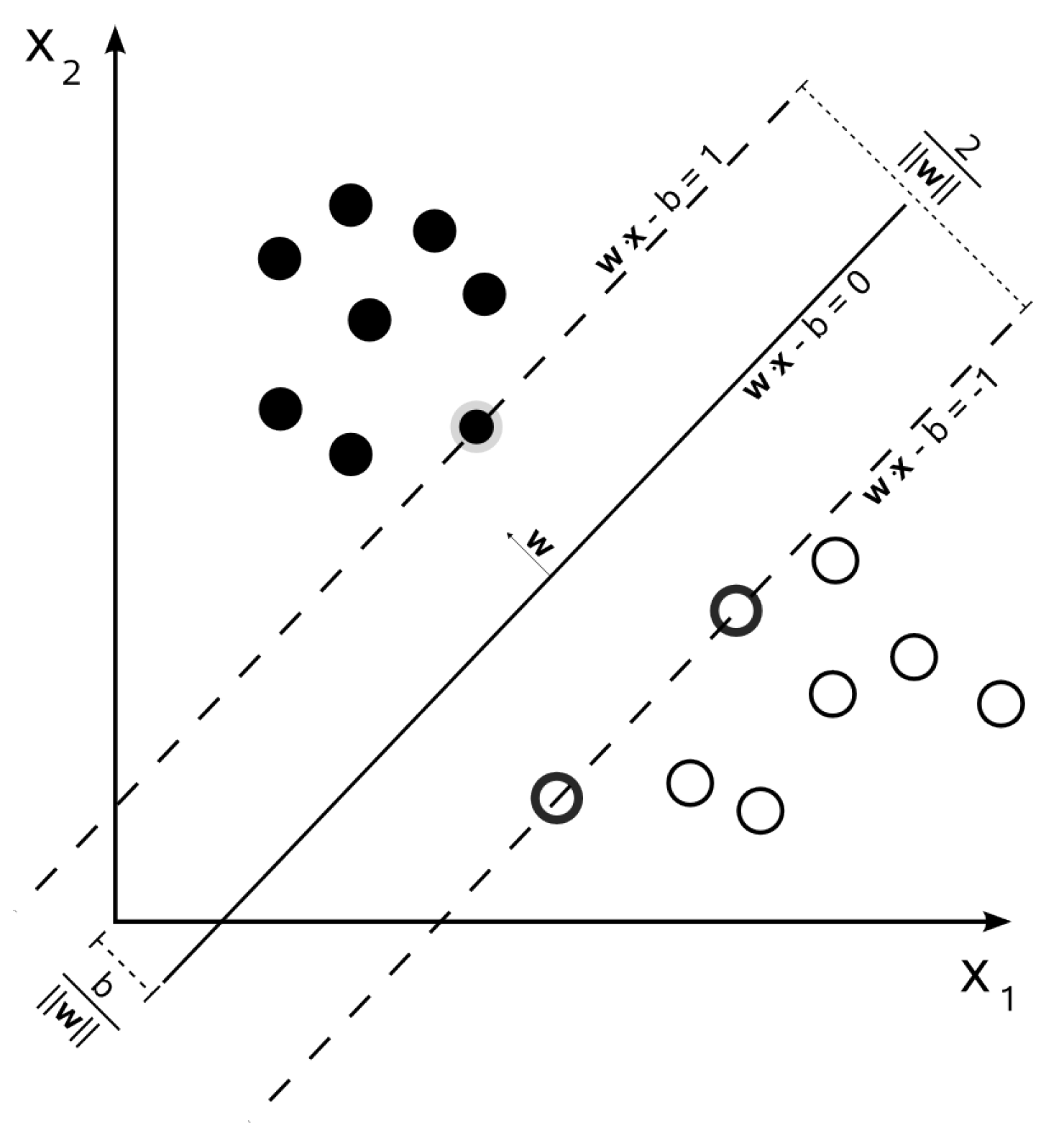
A support vector machine (SVM) system was chosen as the machine learning system. SVM has the advantage that it is simple to visually interpret for a limited number of input parameters. The SVM tries to divide a set of input data into different classes, finding a separation line in the features domain that has the maximum distance from the classes. Figure 4 shows an example taken from the Wikipedia page on SVM [29] of how SVM works for a linear classification. With reference to Figure 4, suppose you have to classify a dot in two different classes (black or white) on the basis of two input features (, ). The SVM computes the separation line by maximizing the distance of the closest elements of two classes, and minimizing the possibility of choosing a separation line that is more favorable to one of the two classes.
The SVM can be extended to a non-linear separation hyperplane by means of kernel functions, multi-dimensional feature arrays, and multi-class classification. Detailed information can be found in several books on SVM (e.g., [22,30,31,32]).
The core part of a machine learning tool is the definition of the input feature array. The number of features has to be reduced in order to avoid computational burden, but indeed it has to be significant to characterize the different classes into which the data should be divided. In the literature, several parameters have been proposed for the condition monitoring of ball bearings [23,25,33]. In this paper, three time-domain parameters are taken as input feature arrays: root mean square (RMS), skewness, and kurtosis of the vibration signal. These parameters characterize the probability distribution of a real-valued random variable. Santos et al. [27] use RMS, skewness, and kurtosis to train SVMs and ANNs (artificial neural networks) for faulted bearing diagnosis at different constant speeds in the case of wind turbines with meaningful results.
For a zero-mean input signal, RMS is equal to the uncorrected sample standard deviation. For a discrete signal , RMS is defined as follows:
Skewness measures the asymmetry of the probability distribution, and is defined as the third standardized moment:
where is the standard deviation of the input data.
Kurtosis measures the tailedness of the probability distribution, and it is defined as the fourth standardized moment:
It has been proved that higher values of kurtosis are related to the presence of impacts in the vibration signal of a faulted bearing [5,34].
The feature array was limited to these three parameters because their effectiveness was proved by the SVM results in constant speed tests, as will be shown in the next section.
3. Results
This section shows the results of the experimental activity and the application of SVM for the diagnostics of ball bearings divided into three classes: healthy, outer race faulted, and inner race faulted. It is divided into five subsections, covering different effects of dynamics on the results of SVM:
- Influence of motion profile on the SVM output;
- Influence of discretization of the speed range in the training step;
- Influence of the length of the signal in the training step;
- Influence of feature arrays in the training step;
- Influence of feature domain in the training step.
The data available were 10 motion profiles (8 constant speed tests, 1 linear speed test, and 1 polynomial speed test, as described in Section 2.2), 2 repetitions, and 3 classes of bearings for a total of 60 samples, each one lasting at least 15 s. To increase the number of data for the training and testing steps, the 15-s samples were divided into sub-segments of 1 s each, obtaining a final dataset of 900 samples.
The reference condition was an SVM trained only on constant speed data, since this is the most common condition investigated in the literature [35,36]. Constant speed data covered the whole speed range considered (10 to 60 Hz) but in discrete steps of 10 Hz. The commercial toolbox we used tried different kernel functions, using 80% of the input data for the training step and the remaining 20% for the test. In all the trials, the best SVM was a fine Gaussian SVM that uses a Gaussian basis function as kernel. More information is available in Ref. [37]. Both healthy and faulted bearings data were provided to the SVM in the training step.
3.1. Influence of Motion Profile
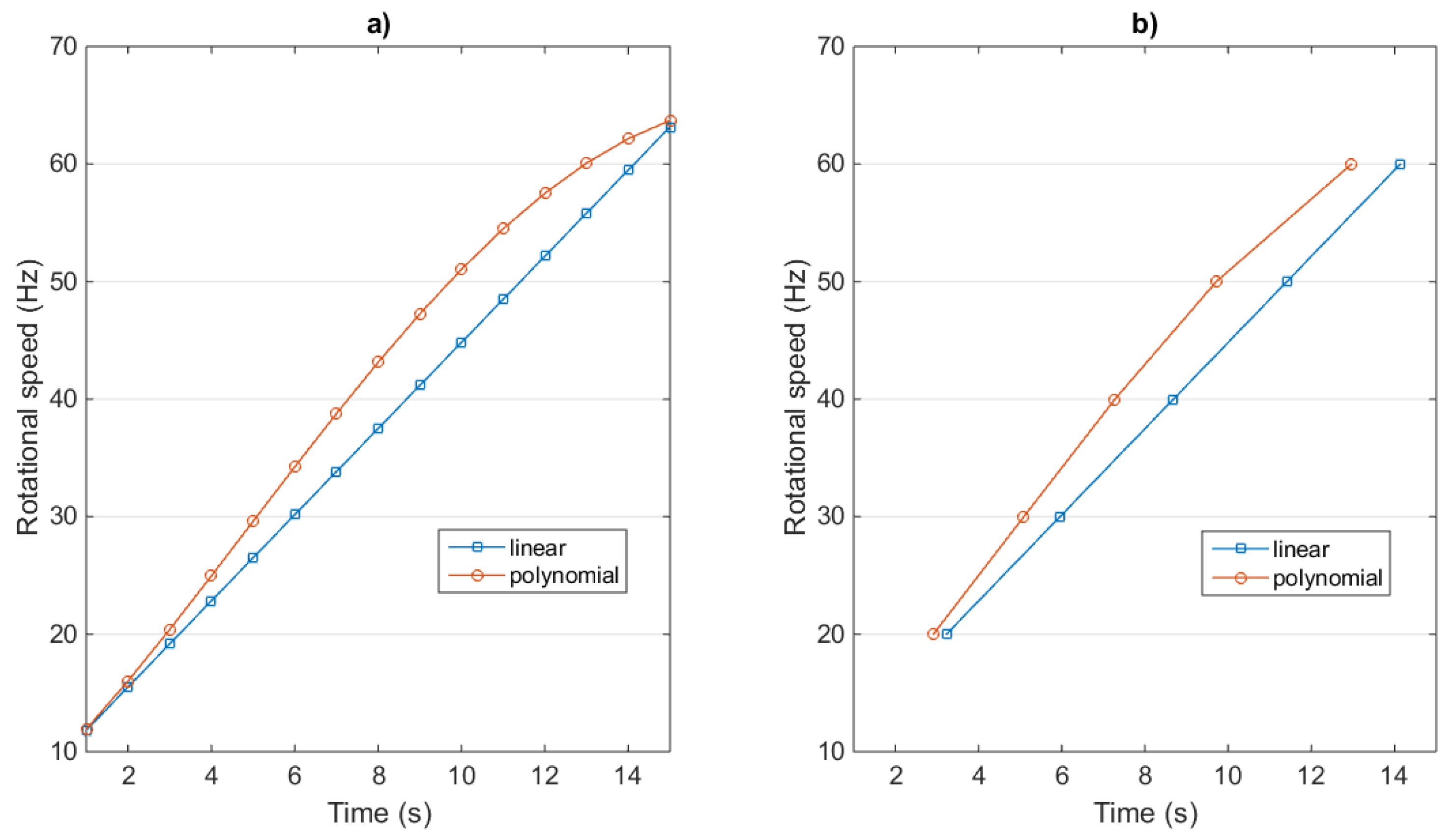
In this test, the SVM applied for the reference condition was used to classify data at variable speeds. The testing data were pre-processed in two different modes. In the first mode, data were split into consecutive 1-s segments. Figure 5a shows the mean speed of each data segment for the linear and polynomial motion profiles. The thin horizontal grid lines refer to the constant speed values used in the training step.
The accuracy of the SVM classification is reported in Table 2. The table lists the number of samples used for the training and testing steps, the accuracy for each motion profile type, and the speed range covered.
In the training step, the SVM was computed on 432 samples at constant speeds. The testing on 108 samples at constant speeds returned 99.5% accuracy, proving the robustness of the SVM and the feature array used. The accuracy dramatically decreased to 57.3% in the classification of 96 samples at the linear speed, and to 51.1% in the classification of 90 samples at the polynomial speed.
A possible cause of the worsening of the SVM results could be the variability of the speed within each sample. Depending on the motion profile, there was a change for the speed of the motor within 1 s that could affect the computed features.
The test was repeated with a different pre-processing mode. Data were still split into non-consecutive 1-s segments. The 1-s samples were chosen to have a mean speed equal to the one used in the training step. Figure 5b clearly shows the mean speed of the new segments. Now the markers correspond with the horizontal grid lines referring to the constant speed values used in the training step. From Table 2, the accuracy of the SVM increased to 75% in the classification of 36 samples at the linear speed, and to 69.4% in the classification of 36 samples at the polynomial speed. The number of samples used was lower than in the previous pre-processing mode since the minimum (maximum) mean-speed values were higher (lower) than some values tested at constant speeds.
The influence of the motion profile test proved the importance of the dynamics of the system in the accuracy of the SVM. The results showed that there was an influence of the mean speed of the input data: the closer it was to the values used in training step, the higher the accuracy of the SVM. However, the results also showed that there was a limit to the accuracy improvement. The test at the same mean speed used in the training stated the influence of the speed profile of the machine. The speed variation within the samples and the kinetic state of the machine made it difficult to use a machine learning technique trained in different working conditions.
3.2. Influence of Discretization of the Speed Range
In this test, three SVMs were created on the basis of a different discretization of the speed range. In particular, the range [10–60] Hz was discretized by steps of 10 and 20 Hz. The range [55–65] Hz was discretized by 5 Hz steps. The difference of the speed range was based on available data. In particular, data were taken in two separate experimental campaigns, with different speed range and discretization step. The aim of this test was to research the correlation between a more detailed span of the speed range and the classification accuracy of the SVMs. Table 3 shows the accuracy of the SVMs.
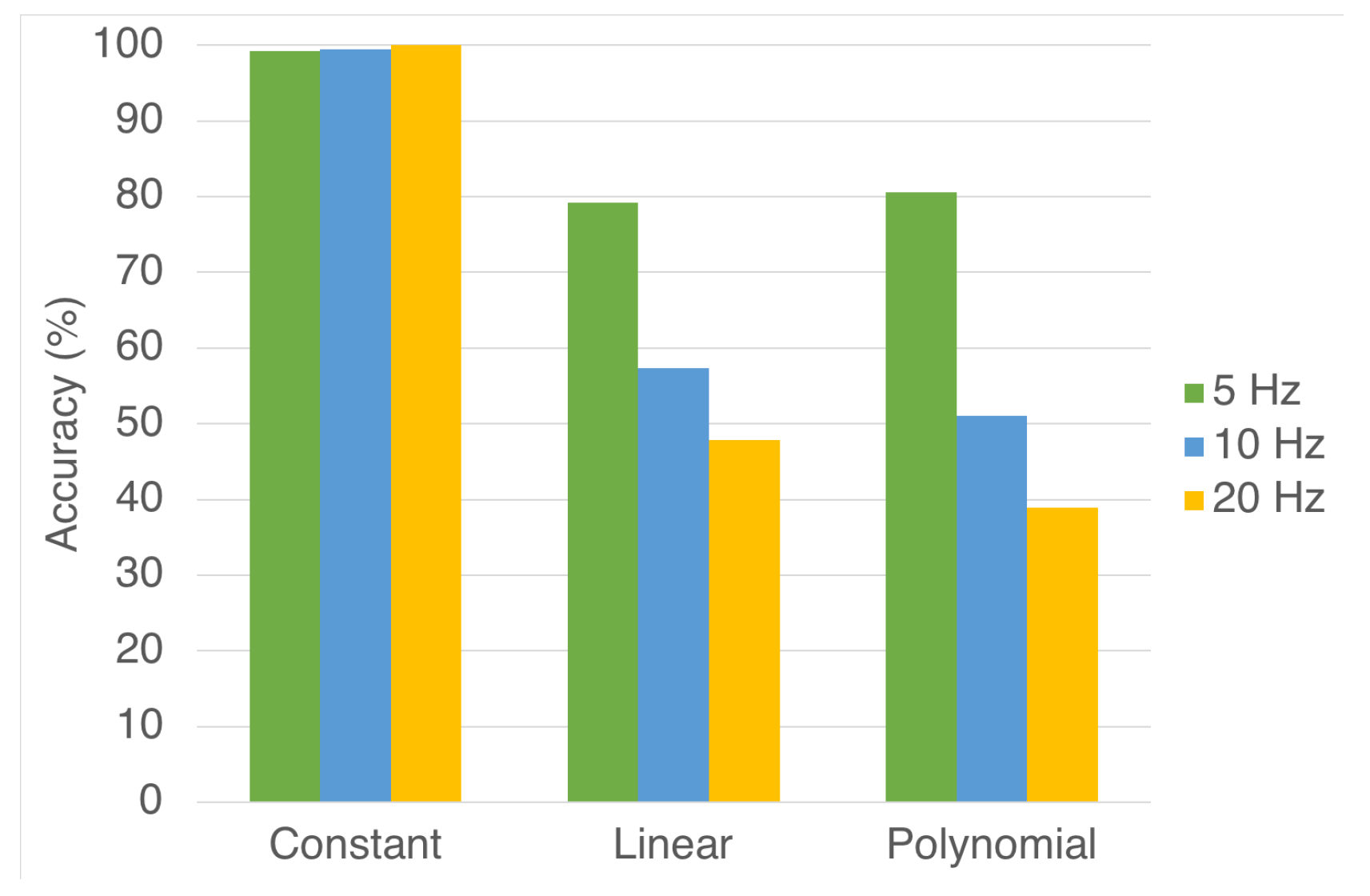
As expected, the effect of discretization of the speed range in the training step was evident. The accuracy of the resulting SVMs was high for the data at constant speeds, since the working conditions were the same used in the training step. The classification accuracy for the variable speed data seemed inversely proportional to the discretization step. For linear speed data, the accuracy fell from 79.2% (5 Hz discretization step) to 57.3% (10 Hz) and 47.9% for 20 Hz steps. For polynomial speed data, the results started from 80.6% (5 Hz) to 51.1% (10 Hz) to 38.9% (20 Hz). This test proved the need for detailed training of the SVMs at all possible speed values. Figure 6 shows a graphical trend of the accuracy results given in Table 3.
3.3. Influence of the Length of the Signal
In this test, three SVMs were created on the basis of different lengths of the signal used in training step. In particular, the acquired data were split into consecutive segments of 0.5, 1, and 1.5 s, respectively. The speed range was [10–65] Hz, and its discretization was equal to 10 Hz. The aim of this test was to research the effect of speed variations within the data used for the computation of input features. Table 4 shows the accuracy of the SVMs. The SVM was consistent (i.e., it correctly classified the data belonging to the same type of the speed profile in which it was trained (constant speeds)). Accuracy for linear and polynomial profiles was almost the same, close to 66% of accuracy.
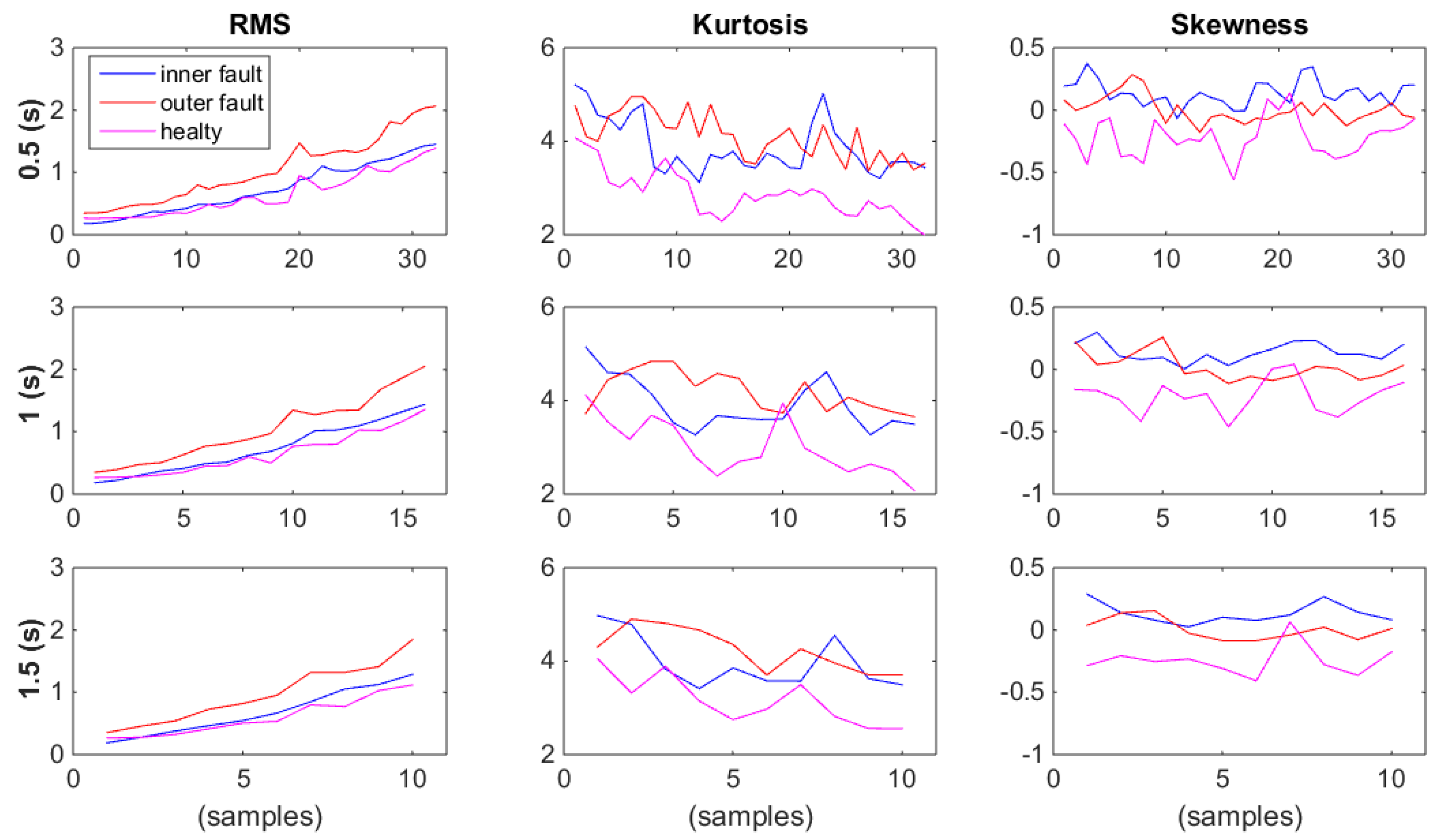
It must be noted that accuracy for the 1-s data was different from the one shown in the previous section. In Section 3.2, the speed covered the [10–60] Hz range with 10 Hz steps, while in this test it was [10–65] Hz, including also 55 Hz and 65 Hz cases. As a consequence, the percentage of success increased. Figure 7 and Figure 8 show variations of feature values for different durations of data input for linear and polynomial profiles, respectively.
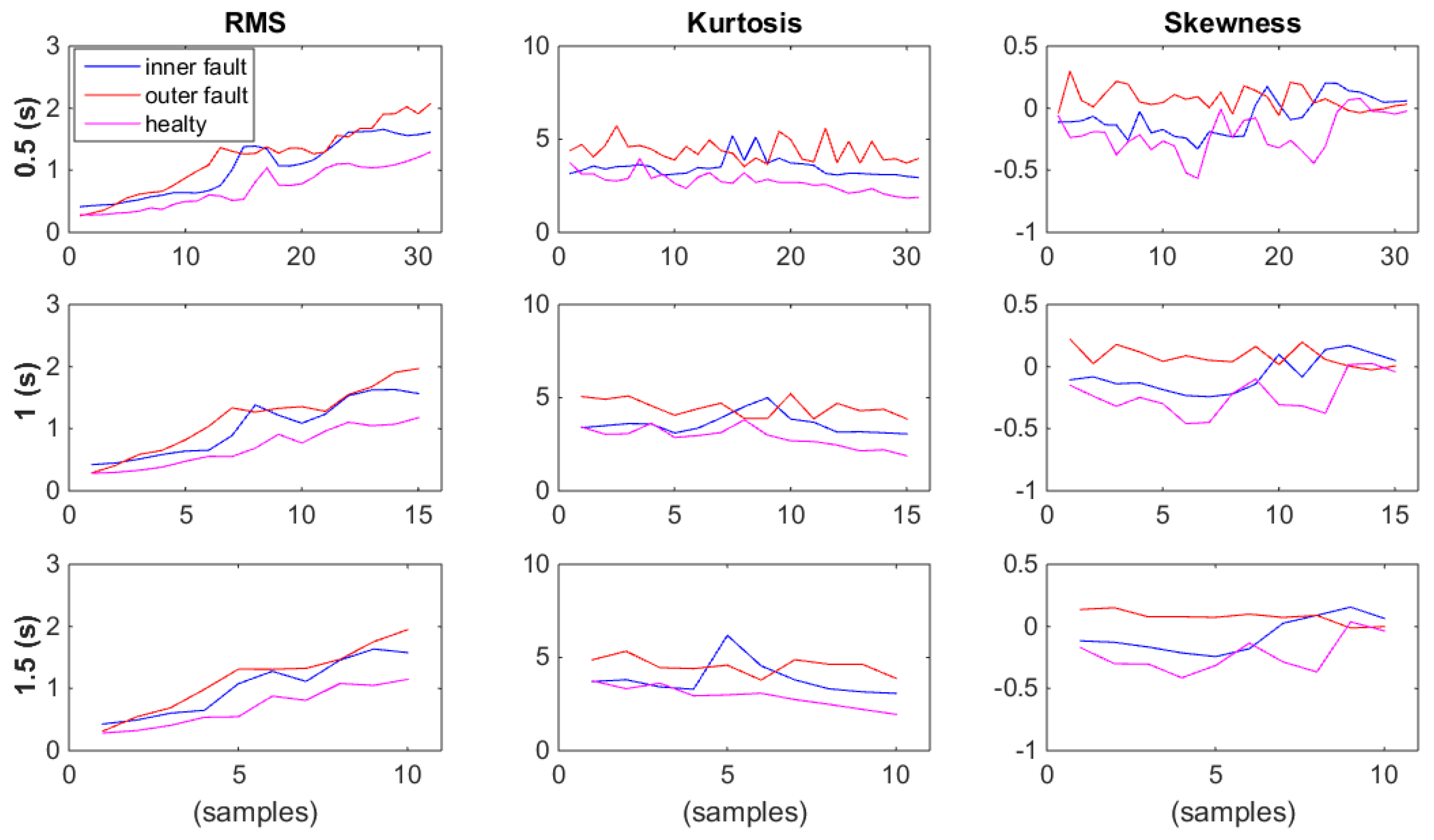
Figure 7 refers to the linear speed motion profile. Each plot corresponds to a specific feature and duration of the data input. In particular, the columns specify the features (RMS, kurtosis, and skewness) and the rows refer to different durations of the input data, in which the features are computed (0.5 s, 1 s, 1.5 s, respectively). The same structure is used in Figure 8, but it is related to the polynomial speed profile. Note that the RMS was the only parameter that detected the speed change, within the test, with a positive increasing trend in all the plots. Figure 7 and Figure 8 show no relevant variations of the feature trend in varying the duration of the input data. This is proved by the accuracy results in Table 4. The percentage of success was almost constant: [62–67]% for the linear speed profile and [67–72]% for the polynomial speed profile.
3.4. Influence of Feature Array in Training Step
Figure 7 and Figure 8 clearly show that RMS brought information regarding the kinetic state of the machine. RMS values increased when the motor speed increased from 10 to 65 Hz. On the contrary, the kurtosis and skewness trends remained almost constant in linear and polynomial speed profiles. It is questionable if the different behavior of the features influenced the SVM accuracy. In this test, different combinations of the three input features were compared. The speed range was [10–65] Hz with steps of 10 Hz. The input data—on the basis of which the features were computed—were consecutive signals of 1-s duration. Table 5 shows the results for the different feature arrays. Using just two feature inputs, the resulting accuracy was always lower than in the three features array case, although the difference was a few percentage points.
3.5. Influence of Features Domain
In this section, the domain of the input features is considered. Only time-domain features were used in this paper. It is questionable as to whether frequency-domain features can give better results or if they can be used together with time-domain features. In particular, three new features were considered in frequency-domain [33]: RMS frequency, spectral skewness, and spectral kurtosis. The definition of these features is the same as in Section 2.3, but computed on the spectrum of the vibration signal instead of the time-domain signal. Note that the Parseval’s theorem states that the RMS values computed in time-domain and in frequency-domain are the same [38]. As a consequence, only time-frequency RMS will be used when both time and frequency domain features are used. The accuracies of the SVM for different feature domains are shown in Table 6. The test was performed in the speed range [10–60] Hz with 10 Hz step and 1 s signal length.
With reference to Table 6, the features used are shown below:
- Time domain: RMS, skewness, and kurtosis.
- Frequency domain: frequency RMS, spectral skewness, and spectral kurtosis.
- Time and frequency domains: RMS, skewness, kurtosis, spectral skewness, and spectral kurtosis.
The results show that frequency features improve the accuracy of the SVM at constant speed, if used in addition to time features. This is due to the presence of a specific fault-related component in the spectrum. Unfortunately, in non-stationary conditions there was a smearing of fault frequency components in the spectrum that reduced the accuracy of the SVM. This trend worsened as the dynamics of the system increased, as in the test with polynomial speed. In the case of linear speed, the accuracy of frequency-domain features was close to the time-domain results. Probably, this was due to the presence of the frequency RMS, which had the same informative content as the RMS value computed in the time domain.
4. Conclusions
In this paper, vibration data from an experimental campaign were used to investigate the application of machine learning—in particular a support vector machine—to the diagnostics of ball bearings in non-stationary operations. The aim of the paper was not to suggest a new tool for diagnostics, since the SVM has been applied successfully in the literature. Regarding a test device made of a servo motor, a shaft, and a bearing under test, this paper tries to tackle the question: if I build an SVM that works well in a given speed range, can I trust it if the dynamics of the machine changes within the imposed speed range? Our experimental campaign on an ad-hoc test rig suggests that the effect of dynamics cannot be overlooked. The working conditions in which the SVM was trained influenced the accuracy results in the classification of faulted bearings. Since a machine learning tool often requires historical data for the training, these data have to be properly chosen to guarantee high-accuracy results in the different working conditions. If the application of the methodology with different motion profiles is foreseen, there are some hints suggested by the results shown in this paper:
- The training data must span the speed range in detail, at least 5 Hz steps.
- Despite the speed range discretization step, there is a limit to the accuracy that depends on the motion profile and cannot be exceeded.
- The accuracy is not sensible to the length of the signal on which the feature array is computed (this is valid for the specific feature array discussed in this paper).
- A proper choice of the feature array can decrease the effect of the variation of the motion profile.
- In non-stationary conditions, time-domain features are preferable to frequency-domain features in the diagnostics of ball-bearings.
These hints are strictly valid for applications similar to the one investigated in this paper, but the critical issues can be extended to any variable-speed application.
Author Contributions
Conceptualization, M.C.; Data curation, J.C.C.M.; Formal analysis, J.C.C.M., R.R., and M.C.; Writing—original draft, J.C.C.M., R.R., and M.C.; Writing—review & editing, J.C.C.M., R.R., and M.C.
Funding
This research received no external funding.
Conflicts of Interest
The authors declare no conflict of interest.
References
- Jardine, A.; Lin, D.; Banjevic, D. A review on machinery diagnostics and prognostics implementing condition-based maintenance. Mech. Syst. Signal Process. 2006, 20, 1483–1510. [Google Scholar] [CrossRef]
- El-Thalji, I.; Jantunen, E. A summary of fault modelling and predictive health monitoring of rolling element bearings. Mech. Syst. Signal Process. 2015, 60–61, 252–272. [Google Scholar] [CrossRef]
- Taylor, J.I.; Kirkland, D.W. The Bearing Analysis Handbook: A Practical Guide for Solving Vibration Problems in Bearings; Vibration Consultants: New York, NY, USA, 2004. [Google Scholar]
- Randall, R.; Antoni, J. Rolling element bearing diagnostics—A tutorial. Mech. Syst. Signal Process. 2011, 25, 485–520. [Google Scholar] [CrossRef]
- Antoni, J. The spectral kurtosis: A useful tool for characterising nonstationary signals. Mech. Syst. Signal Process. 2006, 20, 282–307. [Google Scholar] [CrossRef]
- Antoni, J.; Randall, R. The spectral kurtosis: Application to the vibratory surveillance and diagnostics of rotating machines. Mech. Syst. Signal Process. 2006, 20, 308–331. [Google Scholar] [CrossRef]
- Peng, Z.; Chu, F. Application of the wavelet transform in the condition monitoring and fault diagnostics: A review with bibliograpy. Mech. Syst. Signal Process. 2004, 18, 199–221. [Google Scholar] [CrossRef]
- Donoho, D.; Johnstone, I. Ideal spatial adaptation by wavelet shrinkage. Biometrika 1994, 81, 425–455. [Google Scholar] [CrossRef] [Green Version]
- Antoni, J.; Randall, R. Differential diagnosis of gear and bearing faults. J. Vib. Acoust. 2002, 124, 165–171. [Google Scholar] [CrossRef]
- Antoni, J.; Randall, R. A stochastic model for simulation and diagnostics of rolling element bearings with localized faults. J. Vib. Acoust. 2002, 125, 282–289. [Google Scholar] [CrossRef]
- Chaturvedi, G.H.; Thomas, D.W. Adaptive noise cancelling and condition monitoring. J. Sound Vib. 1981, 76, 391–405. [Google Scholar] [CrossRef]
- McFadden, F. A revised model for the extraction of periodic waveforms by time domain averaging. Mech. Syst. Signal Process. 1987, 1, 83–95. [Google Scholar] [CrossRef]
- Antoni, J.; Randall, R. Unsupervised noise cancellation for vibration signals: Part I—Evaluation of adaptive algorithms. Mech. Syst. Signal Process. 2004, 18, 89–101. [Google Scholar] [CrossRef]
- Antoni, J.; Randall, R. Unsupervised noise cancellation for vibration signals: Part II—A novel frequency-domain algorithm. Mech. Syst. Signal Process. 2004, 18, 103–117. [Google Scholar] [CrossRef]
- Potter, R. A new order tracking method for rotating machinery. Sound Vib. 1990, 24, 30–34. [Google Scholar]
- Cocconcelli, M.; Bassi, L.; Secchi, C.; Fantuzzi, C.; Rubini, R. An algorithm to diagnose ball bearing faults in servomotors running arbitrary motion profiles. Mech. Syst. Signal Process. 2012, 27, 667–682. [Google Scholar] [CrossRef]
- Cocconcelli, M.; Zimroz, R.; Rubini, R.; Bartelmus, W. STFT based approach for ball bearing fault detection in a varying speed motor. In Condition Monitoring of Machinery in Non-Stationary Operation; Fakhfakh, T., Bartelmus, W., Chaari, F., Zimroz, R., Haddar, M., Eds.; Springer: New York, NY, USA, 2012; pp. 41–50. [Google Scholar]
- Worden, K.; Staszewski, W.; Hensman, J. Natural computing for mechanical systems research: A tutorial overview. Mech. Syst. Signal Process. 2011, 25, 4–11. [Google Scholar] [CrossRef]
- Jack, L.; Nandi, A. Fault detection using Support Vector Machines and Artificial Neural Networks, augmented by Genetic Algorithms. Mech. Syst. Signal Process. 2002, 16, 373–390. [Google Scholar] [CrossRef]
- Yang, J.; Zhang, Y.; Zhu, Y. Intelligent fault diagnosis of rolling element bearing based on SVMs and fractal dimension. Mech. Syst. Signal Process. 2007, 21, 2012–2024. [Google Scholar] [CrossRef]
- Konar, P.; Chattopadhyay, P. Bearing fault detection of induction motor using wavelet and Support Vector Machines (SVMs). Appl. Soft Comput. 2011, 11, 4203–4211. [Google Scholar] [CrossRef]
- Vapnik, V. The Nature of Statistical Learning Theory; Springer: New York, NY, USA, 1995. [Google Scholar]
- Widodo, A.; Yang, B. Support vector machine in machine condition monitoring and fault diagnosis. Mech. Syst. Signal Process. 2007, 21, 2560–2574. [Google Scholar] [CrossRef]
- Lui, R.; Yang, B.; Zio, E.; Chen, X. Artificial intelligence for fault diagnosis of rotating machinery: A review. Mech. Syst. Signal Process. 2018, 108, 33–47. [Google Scholar]
- Cerrada, M.; Sanchez, R.; Li, C.; Pacheco, F.; Cabrera, D.; de Oliveira, J.; Vasquez, R. A review on data-driven fault severity assessment in rolling bearing. Mech. Syst. Signal Process. 2018, 99, 169–196. [Google Scholar] [CrossRef]
- Zhou, S.; Qian, S.; Chang, W.; Xiao, Y.; Chen, Y. A novel bearing multi-fault diagnosis approach based on Weighted Permutation Entropy and an Improved SVM Ensemble Classifier. Sensors 2018, 18, 1934. [Google Scholar] [CrossRef] [PubMed]
- Santos, P.; Villa, L.F.; Reñones, A.; Bustillo, A.; Maudes, J. An SVM-Based Solution for Fault Detection in Wind Turbines. Sensors 2015, 15, 5627–5648. [Google Scholar] [CrossRef] [PubMed] [Green Version]
- Biagiotti, L.; Melchiorri, C. Trajectory Planning for Automatic Machines and Robots; Springer: Berlin/Heidelberg, Germany, 2008. [Google Scholar]
- Wikipedia Contributors. Support Vector Machine—Wikipedia, The Free Encyclopedia. 2018. Available online: https://en.wikipedia.org/wiki/Support_vector_machine (accessed on 29 August 2018).
- Cristianini, N.; Shawe-Taylor, J. An Introduction to Support Vector Machines and Other Kernel-Based Learning Methods; Cambridge University Press: New York, NY, USA, 2000. [Google Scholar]
- Crammer, K.; Singer, Y. On the Algorithmic Implementation of Multiclass Kernel-based Vector Machines. J. Mach. Learn. Res. 2001, 2, 265–292. [Google Scholar]
- Scholkopf, B.; Burges, C.; Smola, A. Advances in Kernel Methods: Support Vector Learning; MIT Press: Cambridge, MA, USA, 1999. [Google Scholar]
- Caesarendra, W.; Tjahjowidodo, T. A Review of Feature Extraction Methods in Vibration-Based Condition Monitoring and Its Application for Degradation Trend Estimation of Low-Speed Slew Bearing. Machines 2017, 5, 21. [Google Scholar] [CrossRef]
- Wang, Y.; Xian, J.; Markert, R.; Liang, M. Spectral kurtosis for fault detection, diagnosis and prognostics of rotating machines: A review with applications. Mech. Syst. Signal Process. 2016, 66, 679–698. [Google Scholar] [CrossRef]
- Ruiz-Gonzalez, R.; Gomez-Gil, J.; Gomez-Gil, F.; Martínez-Martínez, V. An SVM-Based Classifier for Estimating the State of Various Rotating Components in Agro-Industrial Machinery with a Vibration Signal Acquired from a Single Point on the Machine Chassis. Sensors 2014, 14, 20713–20735. [Google Scholar] [CrossRef] [PubMed] [Green Version]
- Poyhonen, S.; Negrea, M.; Arkkio, A.; Hyotyniemi, H.; Koivo, H. Fault Diagnostics of an Electrical Machine with Multiple Support Vector Classifiers. In Proceedings of the 2002 IEEE International Symposium on Intelligent Control, Vancouver, BC, Canada, 27–30 October 2002; pp. 373–378. [Google Scholar]
- The MathWorks, Inc. Statistics and Machine Learning Toolbox. User’s Guide; The MathWorks, Inc.: Natick, MA, USA, 2018. [Google Scholar]
- Weisstein, E.W. Parseval’s Theorem. 2018. Available online: http://mathworld.wolfram.com/ParsevalsTheorem.html (accessed on 14 October 2018).
Figure 1.
Test rig. From left to the right: the electric motor, the elastic coupling, the main shaft, its support, and the custom case with the bearing under test. The loading system is in the lower part of the custom case, the mono-axial accelerometer is in the higher part.
Figure 1.
Test rig. From left to the right: the electric motor, the elastic coupling, the main shaft, its support, and the custom case with the bearing under test. The loading system is in the lower part of the custom case, the mono-axial accelerometer is in the higher part.
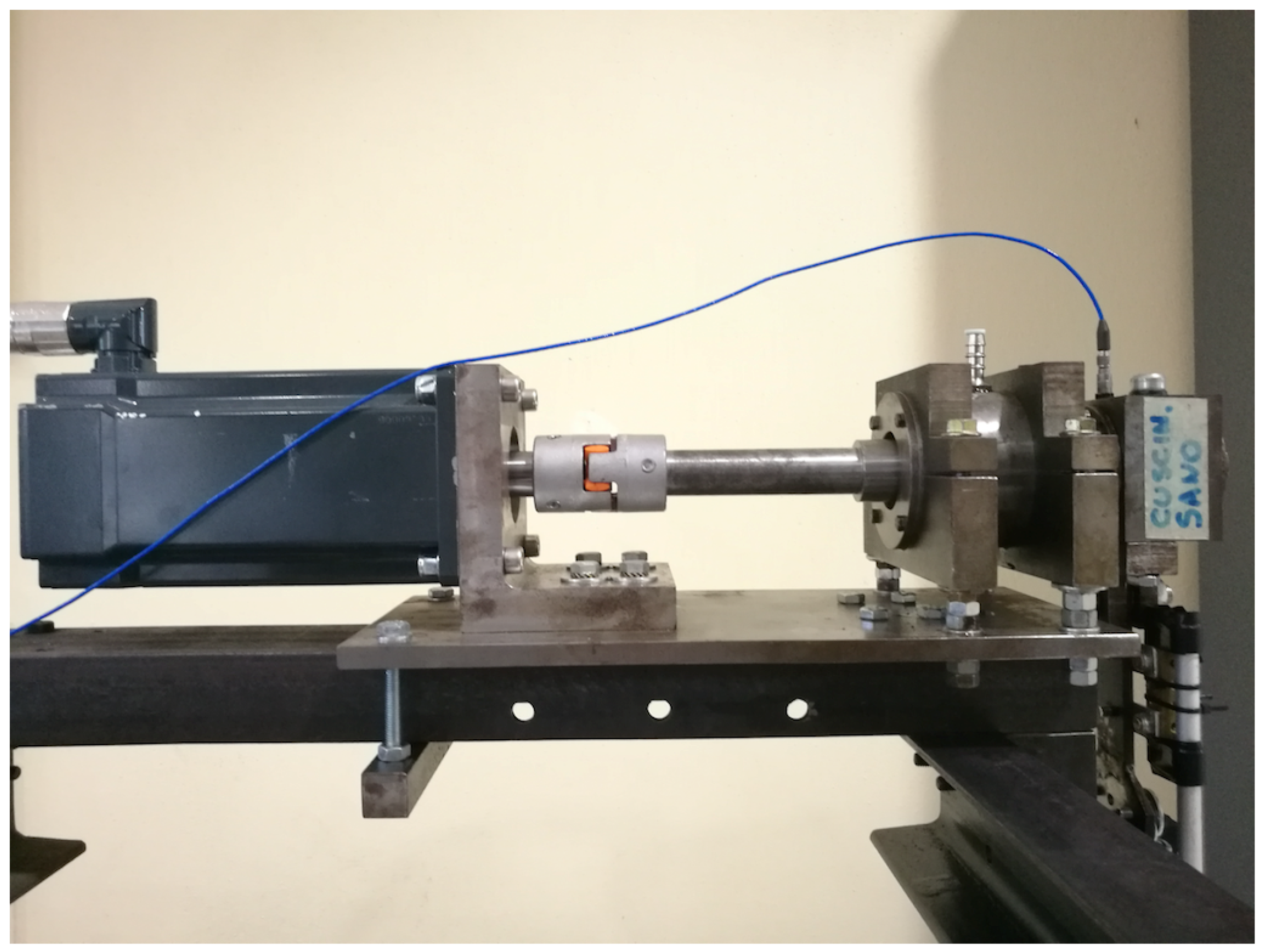
Figure 2.
Raw data (left) and corresponding spectrum (right) for faulted and healthy bearings. The text arrows point to fault frequencies and rotation frequency.
Figure 2.
Raw data (left) and corresponding spectrum (right) for faulted and healthy bearings. The text arrows point to fault frequencies and rotation frequency.
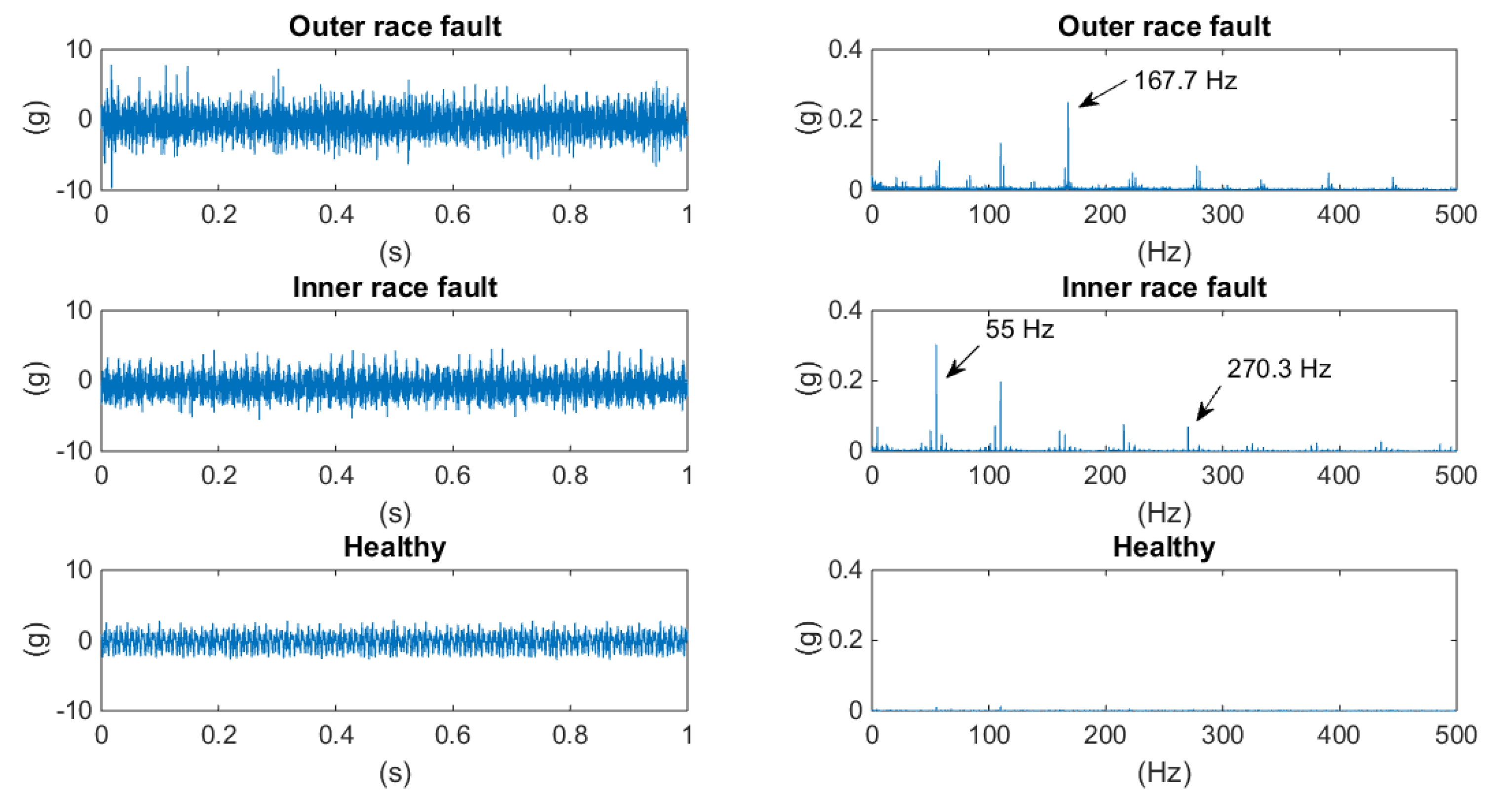
Figure 3.
Speed profiles used in the tests. Solid lines show the three main types: constant, linear, and polynomial. Dotted lines refer to the different values of the constant speeds used.
Figure 3.
Speed profiles used in the tests. Solid lines show the three main types: constant, linear, and polynomial. Dotted lines refer to the different values of the constant speeds used.

Figure 4.
Example of a support vector machine (SVM) for the classification of two classes [29].
Figure 4.
Example of a support vector machine (SVM) for the classification of two classes [29].

Figure 5.
(a) The mean speed of the dataset used considering consecutive 1-s windowing; (b) The mean speed of the dataset used shifting 1-s windowing to get the same mean speed.
Figure 5.
(a) The mean speed of the dataset used considering consecutive 1-s windowing; (b) The mean speed of the dataset used shifting 1-s windowing to get the same mean speed.

Figure 6.
Classification accuracy of the SVMs as a function of the discretization step of the speed range.
Figure 6.
Classification accuracy of the SVMs as a function of the discretization step of the speed range.

Figure 7.
Variations of feature values for different duration of data input for linear speed tests. RMS: root mean square.
Figure 7.
Variations of feature values for different duration of data input for linear speed tests. RMS: root mean square.

Figure 8.
Variations of feature values for different duration of data input for polynomial speed tests.
Figure 8.
Variations of feature values for different duration of data input for polynomial speed tests.


Table 1.
Dimensions of the bearings and characteristic fault frequencies.
| Deep Groove Ball Bearing (6204) | |
|---|---|
| Pitch diameter (mm) | 33.5 |
| Ball diameter (mm) | 7.94 |
| Rotational frequency (Hz) | 55 |
| Outer race fault frequency (Hz) | 167.9 |
| Inner race fault frequency (Hz) | 272.1 |
Table 2.
Accuracy of the SVM with respect to the motion profile.
| Speed Range (Hz) | Samples | Motion Profile | Accuracy | |
|---|---|---|---|---|
| Training | [10, 20, 30, 40, 50, 60] | 432 | Constant | — |
| Test | [10, 20, 30, 40, 50, 60] | 108 | Constant | 99.5% |
| [10–60] (Figure 5a) | 96 | Linear | 57.3% | |
| 90 | Polynomial | 51.1% | ||
| [20, 30, 40, 50, 60] (Figure 5b) | 36 | Linear | 75% | |
| 36 | Polynomial | 69.4% |
Table 3.
Accuracy of the SVMs with respect to discretization of the speed range.
| Δ(Hz) | Speed Range (Hz) | Constant Speed | Linear Speed | Polynomial Speed |
|---|---|---|---|---|
| 5 | [50–65] | 99.3% | 79.2% | 80.6% |
| 10 | [10–60] | 99.5% | 57.3% | 51.1% |
| 20 | [10–50] | 100% | 47.9% | 38.9% |
Table 4.
Accuracy of the SVM with respect to the length of the signal.
| T(s) | Constant Speed | Linear Speed | Polynomial Speed |
|---|---|---|---|
| 0.5 | 99.1% | 64.1% | 68.3% |
| 1 | 100% | 66.7% | 66.7% |
| 1.5 | 99% | 61.7% | 71.7% |
Table 5.
Accuracy of the SVM with different feature arrays.
| Feature Array | Constant Speed | Linear Speed | Polynomial Speed |
|---|---|---|---|
| RMS, kurtosis, skewness | 100% | 66.7% | 66.7% |
| Kurtosis, skewness | 92.7% | 64.6% | 58.9% |
| RMS, kurtosis | 96.2% | 60.42% | 65.56% |
| RMS, skewness | 95.8% | 63.54% | 62.22% |
Table 6.
Accuracy of the SVM with different feature domains.
| Features Domain | Constant Speed | Linear Speed | Polynomial Speed |
|---|---|---|---|
| Time domain | 99.5% | 57.3% | 51.1% |
| Frequency domain | 99.5% | 53.13% | 37.78% |
| Time and frequency domains | 100% | 41.67% | 35.56% |
© 2018 by the authors. Licensee MDPI, Basel, Switzerland. This article is an open access article distributed under the terms and conditions of the Creative Commons Attribution (CC BY) license (http://creativecommons.org/licenses/by/4.0/).
Share and Cite
MDPI and ACS Style
Cavalaglio Camargo Molano, J.; Rubini, R.; Cocconcelli, M. Experimental Evidence of the Speed Variation Effect on SVM Accuracy for Diagnostics of Ball Bearings. Machines 2018, 6, 48. https://doi.org/10.3390/machines6040048
AMA Style
Cavalaglio Camargo Molano J, Rubini R, Cocconcelli M. Experimental Evidence of the Speed Variation Effect on SVM Accuracy for Diagnostics of Ball Bearings. Machines. 2018; 6(4):48. https://doi.org/10.3390/machines6040048
Chicago/Turabian StyleCavalaglio Camargo Molano, Jacopo, Riccardo Rubini, and Marco Cocconcelli. 2018. "Experimental Evidence of the Speed Variation Effect on SVM Accuracy for Diagnostics of Ball Bearings" Machines 6, no. 4: 48. https://doi.org/10.3390/machines6040048
Note that from the first issue of 2016, this journal uses article numbers instead of page numbers. See further details here.