Article

Insights from Explainable Artificial Intelligence of Pollution and Socioeconomic Influences for Respiratory Cancer Mortality in Italy

1
Dipartimento di Scienze del Suolo, della Pianta e degli Alimenti, Università degli Studi di Bari Aldo Moro, 70126 Bari, Italy
2
Istituto Nazionale di Fisica Nucleare, Sezione di Bari, 70126 Bari, Italy
3
Dipartimento Interateneo di Fisica “M. Merlin”, Università degli Studi di Bari Aldo Moro, 70126 Bari, Italy
4
Dipartimento di Farmacia Scienze del Farmaco, Università degli Studi di Bari Aldo Moro, 70126 Bari, Italy
5
Dipartimento di Biomedicina Traslazionale e Neuroscienze, Università degli Studi di Bari Aldo Moro, 70126 Bari, Italy
*
Author to whom correspondence should be addressed.
J. Pers. Med. 2024, 14(4), 430; https://doi.org/10.3390/jpm14040430
Submission received: 4 March 2024 / Revised: 10 April 2024 / Accepted: 11 April 2024 / Published: 18 April 2024
(This article belongs to the Special Issue Artificial Intelligence and Data Integration in Precision Health)

Abstract

:
Respiratory malignancies, encompassing cancers affecting the lungs, the trachea, and the bronchi, pose a significant and dynamic public health challenge. Given that air pollution stands as a significant contributor to the onset of these ailments, discerning the most detrimental agents becomes imperative for crafting policies aimed at mitigating exposure. This study advocates for the utilization of explainable artificial intelligence (XAI) methodologies, leveraging remote sensing data, to ascertain the primary influencers on the prediction of standard mortality rates (SMRs) attributable to respiratory cancer across Italian provinces, utilizing both environmental and socioeconomic data. By scrutinizing thirteen distinct machine learning algorithms, we endeavor to pinpoint the most accurate model for categorizing Italian provinces as either above or below the national average SMR value for respiratory cancer. Furthermore, employing XAI techniques, we delineate the salient factors crucial in predicting the two classes of SMR. Through our machine learning scrutiny, we illuminate the environmental and socioeconomic factors pertinent to mortality in this disease category, thereby offering a roadmap for prioritizing interventions aimed at mitigating risk factors.

1. Introduction

Success in mapping the human genome has stimulated the complementary concept of the exposome, i.e., the measure of the complete environmental exposure of an individual or a population to their surrounding environment and the study of how those exposures relate to health [1]. Research on the exposome in the context of noncommunicable diseases (NCDs), or diseases that cannot be transferred from one person to the other, is relatively novel and advancing impressively [2]. Although NCDs are associated with a genetic predisposition (the genome), exposure to health-affecting environmental parameters has a strong impact on their risk. With the use of Earth observation data, recent research studies in this field are exploring possible associations of NCDs with environmental parameters to identify relevant factors and prioritize intervention strategies to mitigate their effects, in line with one of the targets of the 2030 United Nations Agenda for Sustainable Development [3], i.e., reducing premature mortality from NCDs.
Among NCDs, respiratory tract cancers, which include tracheal, bronchus, and lung cancer, are the leading causes of cancer death [4], registering the highest age-standardized mortality rate among all cancers [5]. Studies focusing on respiratory diseases and/or cancer using Earth observation data include factors such as air pollution, atmospheric factors, and land surface data in their analysis. They recognize air pollution parameters as important factors, such as NO2 and O3, and identify prominent associations with parameters such as PM 2.5 exposure, asbestos exposure, UV irradiation, and light pollution [6,7,8,9,10,11,12].
In our analysis, we use air quality estimates by the CAMS reanalysis dataset of atmospheric composition [13] and spatial census data at provincial resolution (environmental and socioeconomic variables) to predict standard cancer mortality rates (SMRs) attributable to respiratory tract cancers as provided by the Italian National Institute of Statistics (ISTAT). More specifically, using data from 2019, we estimate the national average SMR and define a binary variable with a value of 1 for provinces with an SMR higher than the average and 0 otherwise. We then use Earth observation and census data to predict this binary variable, comparing the performance of thirteen different models. Finally, we apply an explainable artificial intelligence strategy, thus providing model-agnostic insights into how the best model calculates predictions with the aim of facilitating the determination of feature importance and offering a roadmap for prioritizing interventions [14,15]. Our approach is therefore aimed at contributing to a comprehensive understanding of the relationships between the environment and human health for the specific disease under consideration.
This paper is structured as follows. In Section 2, we describe the input data and the adopted methodologies. More specifically, in Section 2.1, we define our input factors; in Section 2.2, we define our output binary variable; in Section 2.4, we reduce the features of the dataset through a multicollinearity analysis; in Section 2.5, we introduce the 13 machine algorithms and the evaluation metrics used; in Section 2.6, we describe the explainable artificial intelligence approach adopted. In Section 3, we present the results of our analysis that we discuss in Section 4. Finally, in Section 6, we draw our conclusions.

2. Materials and Methods

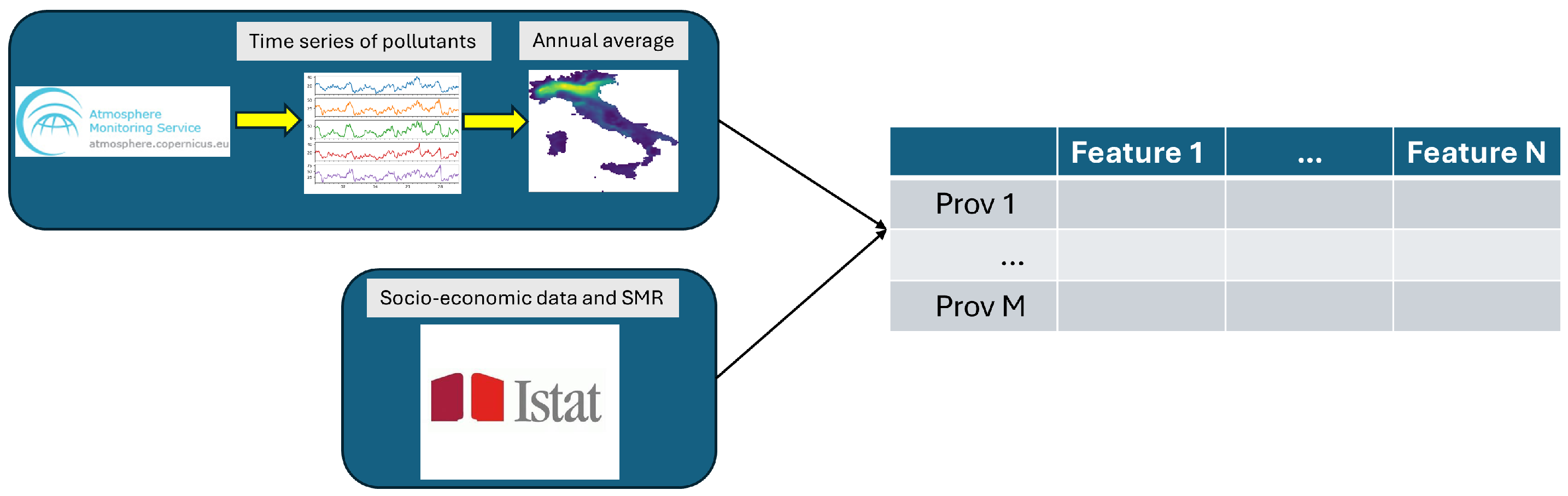
2.1. Pollutants Data and Socioeconomic Indices

The Copernicus Atmosphere Monitoring Service (https://ads.atmosphere.copernicus.eu/#!/search?text=&type=dataset&keywords=((%20%22Product%20type:%20Reanalysis%22%20)%20AND%20(%20%22Variable%20domain:%20Atmosphere%20(composition)%22%20)%20AND%20(%20%22Spatial%20coverage:%20Europe%22%20)%20AND%20(%20%22Temporal%20coverage:%20Past%22%20) (accessed on 10 April 2024) (CAMS) platform managed by the European Union’s Copernicus Program provides information on air pollution and air composition globally. It utilizes data from various sources such as satellites, aircraft, ground stations, and numerical models to monitor and analyze real-time air quality and provide forecasts. The pollutants data provided by the CAMS platform are the result of an ensemble median over 9 numerical air quality models [13,16]: CHIMERE (CH) from INERIS (France) [17], EMEP (EM) from MET Norway (Norway) [18], EURAD-IM (EU) from Jülich IEK (Germany) [19], LOTOS-EUROS (LO) from KNMI and TNO (the Netherlands) [20], MATCH (MA) from SMHI (Sweden) [21], MOCAGE (MO) from Meteo-France (France) [22], SILAM (S) from FMI (Finland) [23], DEHM (DE) from Aarhus University (Denmark) [24], and GEM-AQ (GE) from IEP-NRI (Poland) [25]. For the purposes of the present study, which aims at investigating the association between pollution and mortality for cancer with the respiratory system, only the concentrations of CO, NO, NO2, O3, PM 10, PM 2.5, and SO2 were considered. Since the data downloaded from the CAMS platform covered an area larger than that of our interest, the Python library for analyzing geolocalized data https://geopandas.org/en/stable/ (accessed on 10 April 2024) Geopandas (version 0.14.1) was used to extract the pollution data of the Italian peninsula. From the daily coverage over all of 2019, we retrieved the mean values for the concentrations of the selected pollutants.
In order to maximize data consistency, other pollution-related and socioeconomic variables were considered: cultivated areas, urban areas, benzene, temperature, N fertilizer, P4010 fertilizer, microelement fertilizer, organic fertilizer, the number of hospital beds available (bed number), lifetime, income, life quality, instruction, vehicles per km2 of land area (vehicles total), vehicles per km2 of urbanized surface (urban traffic), photovoltaic panel, percentage of urban greenery density on the surface (green urban), electric consumption, exceeding the limits detected following noise checks (noise), and municipal waste collection in tons (wastes) [26].

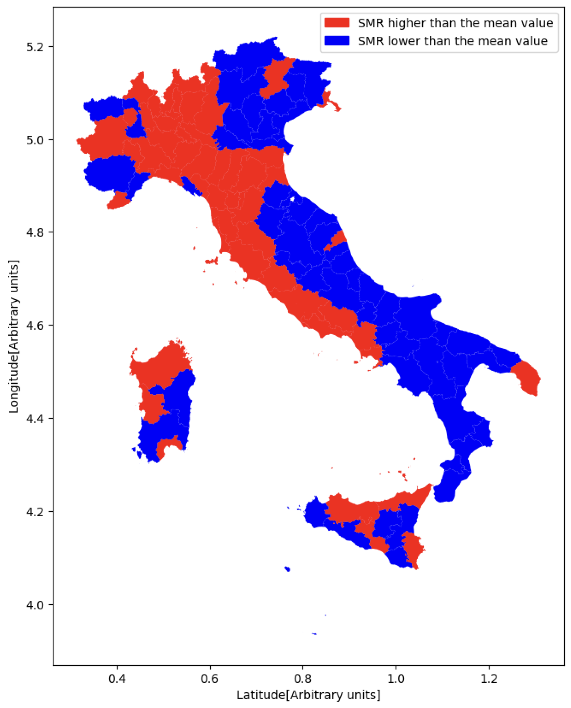
2.2. Standardized Mortality Ratio

The Italian National Institute of Statistics (ISTAT) is the main official statistical institute in Italy, responsible for collecting, analyzing, and disseminating statistical information about the country.
The standardized mortality ratio (SMR) is a measure of the mortality rate of a specific population compared with a standard or reference population (e.g., the national population). It is calculated by dividing the number of observed deaths in the study population by the number of expected deaths based on the mortality rates of the standard population. In our study, the values of the SMR of the Italian provinces were calculated starting from the number of observed deaths for respiratory system cancer in 2019 by age class provided by ISTAT. The mean value of the SMR was used to divide the Italian provinces into two classes: all the provinces with an SMR lower than the mean value were assigned to class 0, while all the others were assigned to class 1. An outline of the data preparation workflow is presented in Figure 1. A graphical representation of Italian provinces with a higher or lower SMR than the mean value for cancer to the respiratory system is shown in Figure 2.

2.3. Analysis Flowchart

The diagram presented in Figure 3 serves as a visual representation encapsulating the comprehensive analytical journey delineated within this paper. At the heart of this endeavor lies the curation of a dataset, meticulously constructed to encompass a rich tapestry of data streams. The foundational pillars of this dataset were erected through a data acquisition process, commencing with the extraction of air pollution metrics from diverse provinces across the Italian peninsula. These statistics were sourced from the Copernicus Atmosphere Monitoring Service (CAMS) platform, renowned for its robust and comprehensive environmental monitoring capabilities. In tandem with air quality metrics, a plethora of socioeconomic indicators were judiciously incorporated into the dataset. These encompassed a spectrum of socioeconomic variables, ranging from income distribution patterns to urbanization indices, providing a holistic perspective on the societal fabric under scrutiny. Furthermore, the dataset was augmented with mortality data attributable to respiratory system cancers, gleaned from the extensive repository maintained by the Italian National Institute of Statistics (ISTAT). The analysis commenced with the exploration of multicollinearity dynamics inherent within the dataset. Leveraging the Variation Inflation Factor (VIF) as a diagnostic tool, we dissected intervariable relationships to discern and mitigate the pernicious effects of collinearity. Through a systematic iterative process, variables exhibiting VIF indices surpassing the critical threshold of 10 were pruned from the dataset, thereby ensuring the integrity and robustness of subsequent analyses. Subsequently, the refined dataset served as fertile ground for the cultivation of predictive models leveraging state-of-the-art machine learning techniques. Employing the Python (3.10.12 version) library https://pycaret.org (accessed on 10 April 2024) PyCaret (version 3.3.0) as a conduit, a diverse ensemble of 13 distinct machine learning models was meticulously trained and fine-tuned and tasked with the classification of provinces exhibiting mortality rates from respiratory system cancers either surpassing or falling below the national average. The efficacy of these predictive models was rigorously scrutinized through a comprehensive validation process, employing a 10-fold cross-validation methodology by evaluating the performance obtained from the validation folds. Once the model with the largest ROC AUC was identified, the most important features for the model to classify provinces with higher or lower mortality due to respiratory system cancer were calculated using the explainable artificial intelligence algorithm SHAP.
Figure 2. Colormap of the Italian provinces with higher or lower SMR than the mean value for cancer to the respiratory system.
Jpm 14 00430 g002
Figure 3. Dataset analysis workflow.
Jpm 14 00430 g003

2.4. Feature Correlation Analysis

The Variation Inflation Factor (VIF) is a measure used in regression analysis to assess multicollinearity among independent variables. The VIF provides an indication of the strength of correlation among independent variables, detecting the effect of inflation on the variance in estimated coefficients in the regression model.
In this study, the VIF was calculated to identify and address the issue of multicollinearity within our dataset. An iterative approach was adopted, where the VIF was computed repeatedly, eliminating the variable with the highest VIF at each iteration, provided its value exceeded the threshold of 10. This process effectively reduced multicollinearity in the model, thereby improving the stability of coefficient estimates.
The surviving features are mean NO, cultivated areas, benzene, P4O10 fertilizer, microelement fertilizer, organic fertilizer, income, instruction, vehicles total, urban traffic, green urban, and noise.

2.5. Comparison of Classification Models

Thirteen different classification models, Gradient Boosting Classifier (gbc) [27], Light Gradient Boosting Machine (lgb) [28], Random Forest Classifier (rf) [29], Extra Trees Classifier (et) [30], K Neighbors Classifier (knn) [31], Extreme Gradient Boosting (xgb) [32], Linear Discriminant Analysis (lda) [33], Ada Boost Classifier (ada) [34], Decision Tree Classifier (dt) [35], Naive Bayes (nb) [36], Quadratic Discriminant Analysis (qda) [37], Logistic Regression (lr) [38], and Dummy Classifier (dum) [39], a classification model that does not learn anything from the training data but is particularly useful for assessing the performance of more complex models and understanding the difficulty of the classification task, were trained on the whole dataset in a 10-stratified cross-validation.
The performance of our machine learning models was evaluated on each validation set through the following metrics:
  • Accuracy:
    A C C = T P + T N T P + F P + T N + F N
  • AUC ROC: The area under the Receiver Operating Characteristic (ROC) curve;
  • Recall:
    R E C = T P T P + F N
  • Precision:
    P R E C = T P T P + F P
  • F1-score:
    F 1 = 2 · P R E C · R E C P R E C + R E C
  • Kappa:
    k = 2 · ( T P · T N F N · F P ) ( T P + F P ) · ( T P + F N ) · ( F N + T N )

2.6. Explainable Algorithm

We adopted the SHAP algorithm [40,41] to explain the decisions of the Gradient Booster Classifier models on each test sample. It provides insight into the contribution of each feature to the model’s prediction for a specific instance. SHAP values are based on game theory concepts and specifically on Shapley values, which originated in cooperative game theory. One of the key advantages of SHAP is its model-agnostic nature. It can be applied to any machine learning model, whether it is a black-box or white-box model, making it versatile and widely applicable. The measurement of how a feature affects the performance of the classification model on the validation set is computed by including and removing it from the model:
Φ j ( x ) = F S { j } | F | ! ( | S | | F | 1 ) ! | S | ! [ f x ( F j ) f x ( F ) ]
where Φ j ( x ) represents the SHAP value of feature j for the prediction of the model f given the input x, S is the set of all features, F S { j } represents all possible subsets of features excluding feature j, and | F | ! ( | S | | F | 1 ) ! | S | ! is a weight parameter that multiplies all of the permutations of S! by the potential permutations of the remaining class that does not belong to S, while f x ( F j ) and f x ( F ) denote, respectively, the model’s prediction when feature j is added to the subset F and when it is absent. We also averaged the ten realizations of SHAP values in order to obtain a single representative SHAP vector. The whole analysis workflow is shown in Figure 3.

3. Results

The aim of this study was to assess, using explainable machine learning models, the extent to which air pollutants and socioeconomic descriptors are associated with higher or lower mortality from respiratory system cancer.

3.1. Performance of Classification Models

Table 1 shows the average performance of the 13 machine learning classifiers calculated as the mean performance obtained during the 10-fold cross-validation. The classifiers are sorted in descending order according to the accuracy values.
The Extra Trees classifier emerged as the best in predicting an SMR higher or lower than the mean value of mortality from respiratory system cancer, with a mean accuracy of 0.74 ± 0.13. The mean ROC AUC of the best model is shown in Figure 4. Each fold of the cross-validation process yielded a distinct AUC value, allowing us to compute the mean AUC across all folds and assess the model’s overall performance.

3.2. Interpreting Model Predictions: Insights from SHAP Analysis

In this section, we present a summary plot of the SHAP values obtained from a binary classification model, shedding light on the influential features driving the model’s predictions. Within the 10-fold cross-validation, SHAP values of the features of the provinces present in the validation fold were calculated after training the classification model with the nine folds of training data. This procedure was repeated for each of the validation folds. The summary plot provides a comprehensive overview of the impact of each feature on model predictions, revealing both the direction and magnitude of their influence. Figure 5 illustrates the summary plot generated from the SHAP values computed for the binary classification model. Each point in the summary plot represents a feature, with its position on the y-axis indicating the feature’s importance in terms of absolute SHAP value. The color of each point represents the feature’s value, with red indicating high values and blue indicating low values. Additionally, the horizontal bars represent the impact of each feature on model predictions, with longer bars signifying a stronger influence.

4. Discussion

Our findings show that most of the input variables included in this study are weakly correlated to the target variable, the standard mortality ratio, while our Extra Trees model accurately predicts provinces withan SMR higher than the mean value. Therefore, it is likely that a nonlinear relationship between air quality and SMR exists, thus suggesting the beneficial role of including machine learning tools in this analysis. This is also consistent when comparing the classification performance of the tree-based algorithms with other shallow classification algorithms, including the LDA (and others). In ecological studies, linear models should be preferred since they are easy to interpret; however, Extra Trees combined with the SHAP is a robust choice that does not require any prior assumptions, while providing local feature importance values that are completely intelligible.
We also used the distribution of the SHAP values as a tool to estimate the global feature importance of the variables included in our analysis. Accordingly, this analysis confirms that average exposure to NOX is the most important feature in predicting the SMR of respiratory system cancer that is higher than the mean value. This result is in agreement with previous analyses confirming the positive association between respiratory diseases and exposure to NO when conducting studies on populations [42,43].
According to this study, the second most important feature was the average benzene concentration per province. Chronic exposure to benzene has been linked to leukemia [44,45]; however, there is limited evidence of a link with respiratory cancer in the scientific literature [45,46,47]. Nevertheless, benzene pollution is typically generated because of biomass combustion due to wildfires [48] and vehicle exhaust [49]. Hence, we believe this variable is a proxy for population exposure to poor air quality due to smoke from combustion from human and natural activities.
Minor effects can also be imputed to microelement fertilizer consumption and extension of the cultivated areas. As can be seen in Figure 5, the distribution of the related SHAP values suggests that these two variables act as a proxy for living in a rural environment.
Another important feature was the mean income per province. Although it is known that socioeconomic inequalities have a role in respiratory cancer outcomes [50], this effect cannot be assessed through a population study. Besides, it is likely that the average income per province is acting as a proxy for residing in high-populated areas, where most of the air pollution is emitted [42], while not accounting for social disparities.

5. Limitations

Key limitations in the proposed workflow stem from the dataset’s limited size and the utilization of standard mortality ratios aggregated at provincial levels to explore associations between respiratory cancer mortality and air pollution. In fact, the dataset’s limited size hampers the ability to discern reliable nonlinear relationships due to the significant influence of outliers and noise. Consequently, we employed a k-fold cross-validation framework and then computed confidence intervals for both predictions and local feature importance. On the other hand, the reliance on aggregated mortality ratios for individual provinces exposes the study to the ecological fallacy, as well as to potential omitted variable bias [51,52], meaning that conclusions drawn at the group level may not accurately represent individual-level associations or causality. Finally, it should be stressed that most of the important variables according to the SHAP algorithm may act as a proxy for the high density of urban activities. If a causality exists, this might be related to the role of NOx in contributing to the development of asthma and respiratory infections, causing a range of harmful effects on lungs [53,54,55]. On the other hand, NO is also related to proximity to residential areas and human activities, so the measured positive association could be partly attributable to other air pollutants, including particulate matter [42]. This work presents a first attempt to extensively evaluate the statistical association between air quality and respiratory cancer mortality over the Italian provinces while accounting for effects from confounding socioeconomic variables. Our conclusions are in agreement with previous cohort studies and meta-analyses [42,56]. The database considered here examined a single year of observations; thus, extending the temporal range of our study could grant increased robustness to the analyses and design a regression approach to model the SMR due to respiratory cancer.

6. Conclusions

This paper explores the intricate relationship between air pollution and respiratory cancer, with a focus on cancers of the lung, trachea, and bronchi. Recognizing the urgent public health challenge posed by respiratory cancers, we address the need to identify the most harmful pollutants to inform targeted policy interventions. Our study introduces a novel approach using explainable artificial intelligence based on remote sensing data and socioeconomic data to predict Italian provinces with respiratory system cancer mortality rates higher or lower than the average, which offers several implications for formulating regulations and allocating resources. The results of the research can provide an empirical basis for adopting or strengthening regulations regarding air quality. Identifying provinces with higher mortality rates for respiratory system cancers can highlight areas with higher levels of air pollution and provide an incentive for implementing policies aimed at reducing atmospheric pollution. The ability to predict provinces with respiratory system cancer mortality rates higher or lower than the average can guide more efficient allocation of resources. Areas identified with higher risk may require additional investments in prevention programs, early diagnosis, and treatment of respiratory system cancer, as well as interventions to improve air quality. The adoption of stricter regulations on air pollution and the targeted allocation of healthcare resources can improve the respiratory health of a population and reduce the incidence and mortality of respiratory system cancers.

Author Contributions

Conceptualization, D.R., R.C. and S.T.; methodology, D.R., P.N., D.D. and S.T.; software, D.R. and D.D.; validation, D.R., P.N., D.D., R.C., E.P., R.B. and S.T.; investigation, D.R. and P.N.; data curation, D.R. and R.C.; writing—original draft preparation, D.R., P.N., R.C., E.P. and S.T.; writing—review and editing, D.R., P.N., D.D., R.C., E.P., N.A., L.B., A.M., R.B. and S.T.; visualization, D.R., D.D., R.C. and S.T.; supervision, S.T. All authors have read and agreed to the published version of the manuscript.

Funding

This paper has been supported by the TEBAKA (TErritorial BAsic Knowledge Acquisition project “Avviso MIUR n.1735 del 13/07/2017”, the National Institute for Nuclear Physics (INFN),next_AIM (Artificial Intelligence in Medicine: next steps) research project (INFN-CSN5), https://www.pi.infn.it/aim (accessed on 30 October 2023); the National Recovery and Resilience Plan(NRRP), Mission 4 Component 2 Investment 1.4—Call for tender No. 3138 of 16 December 2021 of Italian Ministry of University and Research funded by the European Union—NextGenerationEU. Award Number: Project code: CN00000013, Concession Decree No. 1031 of 17 February 2022 adopted by the Italian Ministry of University and Research, CUP H93C22000450007, Project title: “National Centre for HPC, Big Data and Quantum Computing”.

Institutional Review Board Statement

Not applicable.

Informed Consent Statement

Not applicable.

Data Availability Statement

The data that support the findings of this study are either publicly available on databases cited in the bibliography or available from the corresponding author on request.

Acknowledgments

The authors would like to thank the resources made available by ReCaS, a project funded by the MIUR (Italian Ministry for Education, University and Research) in the “PON Ricerca e Competitività 2007–2013-Azione I-Interventi di rafforzamento strutturale” PONa3 _00052, Avviso 254/Ric, University of Bari.

Conflicts of Interest

The authors declare no conflicts of interest.

References

  1. Wild, C.P. The exposome: From concept to utility. Int. J. Epidemiol. 2012, 41, 24–32. [Google Scholar] [CrossRef] [PubMed]
  2. Sogno, P.; Traidl-Hoffmann, C.; Kuenzer, C. Earth observation data supporting non-communicable disease research: A review. Remote Sens. 2020, 12, 2541. [Google Scholar] [CrossRef]
  3. United Nations Department of Economic and Social Affairs. The Sustainable Development Goals Report 2023: Special Edition; United Nations Department of Economic and Social Affairs: New York, NY, USA, 2023. [Google Scholar]
  4. Bray, F.; Ferlay, J.; Soerjomataram, I.; Siegel, R.L.; Torre, L.A.; Jemal, A. Global cancer statistics 2018: GLOBOCAN estimates of incidence and mortality worldwide for 36 cancers in 185 countries. CA Cancer J. Clin. 2018, 68, 394–424. [Google Scholar] [CrossRef] [PubMed]
  5. Mahesh, P. Implementing precision medicine in best practices of chronic airway diseases. Indian J. Med. Res. 2019, 149, 802. [Google Scholar] [CrossRef]
  6. Hystad, P.; Demers, P.A.; Johnson, K.C.; Brook, J.; van Donkelaar, A.; Lamsal, L.; Martin, R.; Brauer, M. Spatiotemporal air pollution exposure assessment for a Canadian population-based lung cancer case-control study. Environ. Health 2012, 11, 22. [Google Scholar] [CrossRef] [PubMed]
  7. Tomczak, A.; Miller, A.B.; Weichenthal, S.A.; To, T.; Wall, C.; van Donkelaar, A.; Martin, R.V.; Crouse, D.L.; Villeneuve, P.J. Long-term exposure to fine particulate matter air pollution and the risk of lung cancer among participants of the Canadian National Breast Screening Study. Int. J. Cancer 2016, 139, 1958–1966. [Google Scholar] [CrossRef] [PubMed]
  8. Consonni, D.; Carugno, M.; De Matteis, S.; Nordio, F.; Randi, G.; Bazzano, M.; Caporaso, N.E.; Tucker, M.A.; Bertazzi, P.A.; Pesatori, A.C.; et al. Outdoor particulate matter (PM10) exposure and lung cancer risk in the EAGLE study. PLoS ONE 2018, 13, e0203539. [Google Scholar] [CrossRef] [PubMed]
  9. Di Gilio, A.; Catino, A.; Lombardi, A.; Palmisani, J.; Facchini, L.; Mongelli, T.; Varesano, N.; Bellotti, R.; Galetta, D.; de Gennaro, G.; et al. Breath analysis for early detection of malignant pleural mesothelioma: Volatile organic compounds (VOCs) determination and possible biochemical pathways. Cancers 2020, 12, 1262. [Google Scholar] [CrossRef] [PubMed]
  10. Kamis, A.; Cao, R.; He, Y.; Tian, Y.; Wu, C. Predicting lung cancer in the United States: A multiple model examination of public health factors. Int. J. Environ. Res. Public Health 2021, 18, 6127. [Google Scholar] [CrossRef]
  11. Ahmed, Z.U.; Sun, K.; Shelly, M.; Mu, L. Explainable artificial intelligence (XAI) for exploring spatial variability of lung and bronchus cancer (LBC) mortality rates in the contiguous USA. Sci. Rep. 2021, 11, 24090. [Google Scholar] [CrossRef]
  12. Monaco, A.; Lacalamita, A.; Amoroso, N.; D’Orta, A.; Del Buono, A.; di Tuoro, F.; Tangaro, S.; Galeandro, A.I.; Bellotti, R. Random forests highlight the combined effect of environmental heavy metals exposure and genetic damages for cardiovascular diseases. Appl. Sci. 2021, 11, 8405. [Google Scholar] [CrossRef]
  13. Casciaro, G.; Cavaiola, M.; Mazzino, A. Calibrating the CAMS European multi-model air quality forecasts for regional air pollution monitoring. Atmos. Environ. 2022, 287, 119259. [Google Scholar] [CrossRef]
  14. Ladbury, C.; Zarinshenas, R.; Semwal, H.; Tam, A.; Vaidehi, N.; Rodin, A.S.; Liu, A.; Glaser, S.; Salgia, R.; Amini, A. Utilization of model-agnostic explainable artificial intelligence frameworks in oncology: A narrative review. Transl. Cancer Res. 2022, 11, 3853. [Google Scholar] [CrossRef] [PubMed]
  15. Roussel, C.; Böhm, K. Geospatial xai: A review. ISPRS Int. J. Geo-Inf. 2023, 12, 355. [Google Scholar] [CrossRef]
  16. Marécal, V.; Peuch, V.H.; Andersson, C.; Andersson, S.; Arteta, J.; Beekmann, M.; Benedictow, A.; Bergström, R.; Bessagnet, B.; Cansado, A.; et al. A regional air quality forecasting system over Europe: The MACC-II daily ensemble production. Geosci. Model Dev. 2015, 8, 2777–2813. [Google Scholar] [CrossRef]
  17. Thunis, P.; Degraeuwe, B.; Pisoni, E.; Meleux, F.; Clappier, A. Analyzing the efficiency of short-term air quality plans in European cities, using the CHIMERE air quality model. Air Qual. Atmos. Health 2017, 10, 235–248. [Google Scholar] [CrossRef] [PubMed]
  18. Hass, H.; Ebel, A.; Feldmann, H.; Jakobs, H.; Memmesheimer, M. Evaluation studies with a regional chemical transport model (EURAD) using air quality data from the EMEP monitoring network. Atmos. Environ. Part Gen. Top. 1993, 27, 867–887. [Google Scholar] [CrossRef]
  19. Duarte, E.D.S.F.; Franke, P.; Lange, A.C.; Friese, E.; da Silva Lopes, F.J.; da Silva, J.J.; dos Reis, J.S.; Landulfo, E.; e Silva, C.M.S.; Elbern, H.; et al. Evaluation of atmospheric aerosols in the metropolitan area of São Paulo simulated by the regional EURAD-IM model on high-resolution. Atmos. Pollut. Res. 2021, 12, 451–469. [Google Scholar] [CrossRef]
  20. Hinestroza-Ramirez, J.E.; Lopez-Restrepo, S.; Yarce Botero, A.; Segers, A.; Rendon-Perez, A.M.; Isaza-Cadavid, S.; Heemink, A.; Quintero, O.L. Improving Air Pollution Modelling in Complex Terrain with a Coupled WRF–LOTOS–EUROS Approach: A Case Study in Aburrá Valley, Colombia. Atmosphere 2023, 14, 738. [Google Scholar] [CrossRef]
  21. Persson, C.; Langner, J.; Robertson, L. Air pollution assessment studies for Sweden based on the MATCH model and air pollution measurements. In Air Pollution Modeling and Its Application XI; Springer: Berlin/Heidelberg, Germany, 1996; pp. 127–134. [Google Scholar]
  22. Joly, M.; Josse, B.; Plu, M.; Arteta, J.; Guth, J.; Meleux, F. High-Resolution Air Quality Forecasts with MOCAGE Chemistry Transport Model. In Air Pollution Modeling and Its Application XXIV; Springer: Berlin/Heidelberg, Germany, 2016; pp. 563–565. [Google Scholar]
  23. Ots, R.; Loot, A.; Kaasik, M. Scale-dependent and seasonal performance of SILAM model in Estonia. In Air Pollution Modeling and its Application XXII; Springer: Berlin/Heidelberg, Germany, 2014; pp. 593–597. [Google Scholar]
  24. Van Loon, M.; Vautard, R.; Schaap, M.; Bergström, R.; Bessagnet, B.; Brandt, J.; Builtjes, P.; Christensen, J.; Cuvelier, C.; Graff, A.; et al. Evaluation of long-term ozone simulations from seven regional air quality models and their ensemble. Atmos. Environ. 2007, 41, 2083–2097. [Google Scholar] [CrossRef]
  25. Neary, L.; Kaminski, J.W.; Lupu, A.; McConnell, J.C. Developments and results from a global multiscale air quality model (GEM-AQ). In Air Pollution Modeling and Its Application XVII; Springer: Berlin/Heidelberg, Germany, 2007; pp. 403–410. [Google Scholar]
  26. Cazzolla Gatti, R.; Di Paola, A.; Monaco, A.; Velichevskaya, A.; Amoroso, N.; Bellotti, R. The spatial association between environmental pollution and long-term cancer mortality in Italy. Sci. Total Environ. 2023, 855, 158439. [Google Scholar] [CrossRef]
  27. Mayr, A.; Binder, H.; Gefeller, O.; Schmid, M. The evolution of boosting algorithms. Methods Inf. Med. 2014, 53, 419–427. [Google Scholar] [PubMed]
  28. Abdurrahman, M.H.; Irawan, B.; Setianingsih, C. A review of light gradient boosting machine method for hate speech classification on twitter. In Proceedings of the 2020 2nd International Conference on Electrical, Control and Instrumentation Engineering (ICECIE), Kuala Lumpur, Malaysia, 28 November 2020; pp. 1–6. [Google Scholar]
  29. Parmar, A.; Katariya, R.; Patel, V. A review on random forest: An ensemble classifier. In International Conference on Intelligent Data Communication Technologies and Internet of Things (ICICI) 2018; Springer: Berlin/Heidelberg, Germany, 2019; pp. 758–763. [Google Scholar]
  30. Baby, D.; Devaraj, S.J.; Hemanth, J. Leukocyte classification based on feature selection using extra trees classifier: Atransfer learning approach. Turk. J. Electr. Eng. Comput. Sci. 2021, 29, 2742–2757. [Google Scholar] [CrossRef]
  31. Kataria, A.; Singh, M. A review of data classification using k-nearest neighbour algorithm. Int. J. Emerg. Technol. Adv. Eng. 2013, 3, 354–360. [Google Scholar]
  32. Azmi, S.S.; Baliga, S. An overview of boosting decision tree algorithms utilizing AdaBoost and XGBoost boosting strategies. Int. Res. J. Eng. Technol. 2020, 7, 6867–6870. [Google Scholar]
  33. McLachlan, G.J. Discriminant analysis. Wiley Interdiscip. Rev. Comput. Stat. 2012, 4, 421–431. [Google Scholar] [CrossRef]
  34. An, T.K.; Kim, M.H. A new diverse AdaBoost classifier. In Proceedings of the 2010 International conference on artificial intelligence and computational intelligence, Sanya, China, 23–24 October 2010; Volume 1, pp. 359–363. [Google Scholar]
  35. Kotsiantis, S.B. Decision trees: A recent overview. Artif. Intell. Rev. 2013, 39, 261–283. [Google Scholar] [CrossRef]
  36. Saritas, M.M.; Yasar, A. Performance analysis of ANN and Naive Bayes classification algorithm for data classification. Int. J. Intell. Syst. Appl. Eng. 2019, 7, 88–91. [Google Scholar] [CrossRef]
  37. Tharwat, A. Linear vs. quadratic discriminant analysis classifier: A tutorial. Int. J. Appl. Pattern Recognit. 2016, 3, 145–180. [Google Scholar] [CrossRef]
  38. Nick, T.G.; Campbell, K.M. Logistic regression. Top. Biostat. 2007, 273–301. [Google Scholar]
  39. Barletta, L.; Giusti, A.; Rottondi, C.; Tornatore, M. QoT estimation for unestablished lighpaths using machine learning. In Optical Fiber Communication Conference; Optica Publishing Group: Washington, DC, USA, 2017; p. Th1J-1. [Google Scholar]
  40. Lundberg, S.M.; Lee, S.I. A unified approach to interpreting model predictions. Adv. Neural Inf. Process. Syst. 2017, 30. [Google Scholar]
  41. Lundberg, S.M.; Erion, G.; Chen, H.; DeGrave, A.; Prutkin, J.M.; Nair, B.; Katz, R.; Himmelfarb, J.; Bansal, N.; Lee, S.I. From local explanations to global understanding with explainable AI for trees. Nat. Mach. Intell. 2020, 2, 56–67. [Google Scholar] [CrossRef] [PubMed]
  42. Hamra, G.B.; Laden, F.; Cohen, A.J.; Raaschou-Nielsen, O.; Brauer, M.; Loomis, D. Lung Cancer and Exposure to Nitrogen Dioxide and Traffic: A Systematic Review and Meta-Analysis. Environ. Health Perspect. 2015, 123, 1107–1112. [Google Scholar] [CrossRef]
  43. Amoroso, N.; Cilli, R.; Maggipinto, T.; Monaco, A.; Tangaro, S.; Bellotti, R. Satellite data and machine learning reveal a significant correlation between NO2 and COVID-19 mortality. Environ. Res. 2022, 204, 111970. [Google Scholar] [CrossRef] [PubMed]
  44. Snyder, R. Leukemia and benzene. Int. J. Environ. Res. Public Health 2012, 9, 2875–2893. [Google Scholar] [CrossRef] [PubMed]
  45. Loomis, D.; Guyton, K.Z.; Grosse, Y.; El Ghissassi, F.; Bouvard, V.; Benbrahim-Tallaa, L.; Guha, N.; Vilahur, N.; Mattock, H.; Straif, K. Carcinogenicity of benzene. Lancet Oncol. 2017, 18, 1574–1575. [Google Scholar] [CrossRef] [PubMed]
  46. Ferrero, A.; Esplugues, A.; Estarlich, M.; Llop, S.; Cases, A.; Mantilla, E.; Ballester, F.; Iñiguez, C. Infants’ indoor and outdoor residential exposure to benzene and respiratory health in a Spanish cohort. Environ. Pollut. 2017, 222, 486–494. [Google Scholar] [CrossRef] [PubMed]
  47. D’Andrea, M.A.; Reddy, G.K. Health Risks Associated With Benzene Exposure in Children: A Systematic Review. Glob. Pediatr. Health 2018, 5, 2333794X18789275. [Google Scholar] [CrossRef] [PubMed]
  48. O’Dell, K.; Hornbrook, R.S.; Permar, W.; Levin, E.J.; Garofalo, L.A.; Apel, E.C.; Blake, N.J.; Jarnot, A.; Pothier, M.A.; Farmer, D.K.; et al. Hazardous air pollutants in fresh and aged western US wildfire smoke and implications for long-term exposure. Environ. Sci. Technol. 2020, 54, 11838–11847. [Google Scholar] [CrossRef]
  49. Jo, W.K.; Song, K.B. Exposure to volatile organic compounds for individuals with occupations associated with potential exposure to motor vehicle exhaust and/or gasoline vapor emissions. Sci. Total Environ. 2001, 269, 25–37. [Google Scholar] [CrossRef]
  50. Redondo-Sánchez, D.; Petrova, D.; Rodríguez-Barranco, M.; Fernández-Navarro, P.; Jiménez-Moleón, J.J.; Sánchez, M.J. Socio-economic inequalities in lung cancer outcomes: An overview of systematic reviews. Cancers 2022, 14, 398. [Google Scholar] [CrossRef] [PubMed]
  51. Wilms, R.; Mäthner, E.; Winnen, L.; Lanwehr, R. Omitted variable bias: A threat to estimating causal relationships. Methods Psychol. 2021, 5, 100075. [Google Scholar] [CrossRef]
  52. Clarke, K.A. The phantom menace: Omitted variable bias in econometric research. Confl. Manag. Peace Sci. 2005, 22, 341–352. [Google Scholar] [CrossRef]
  53. Pilotto, L.S.; Douglas, R.M.; Wilson, S.R. Respiratory effects associated with indoor nitrogen dioxide exposure in children. Int. J. Epidemiol. 1997, 26, 788–796. [Google Scholar] [CrossRef] [PubMed]
  54. Gamble, J.; Jones, W.; Minshall, S. Epidemiological-environmental study of diesel bus garage workers: Acute effects of NO2 and respirable particulate on the respiratory system. Environ. Res. 1987, 42, 201–214. [Google Scholar] [CrossRef] [PubMed]
  55. Kubota, K.; Murakami, M.; Takenaka, S.; Kawai, K.; Kyono, H. Effects of long-term nitrogen dioxide exposure on rat lung: Morphological observations. Environ. Health Perspect. 1987, 73, 157–169. [Google Scholar] [CrossRef]
  56. Atkinson, R.W.; Butland, B.K.; Anderson, H.R.; Maynard, R.L. Long-term concentrations of nitrogen dioxide and mortality: A meta-analysis of cohort studies. Epidemiology 2018, 29, 460. [Google Scholar] [CrossRef]
Figure 1. Dataset construction workflow.
Jpm 14 00430 g001
Figure 4. Average ROC curve with standard deviation of the Extra Trees classifier over 10 validation sets.
Jpm 14 00430 g004
Figure 5. Shap summary plot. It reports the SHAP values, represented along the x-axis, of the dataset features, reported on the y-axis. Each point on the graph represents a province.
Jpm 14 00430 g005
Table 1. Performance of different classification models.
ModelAccuracyAUCRecallPrec.F1Kappa
et0.78 ± 0.190.75 ± 0.170.73 ± 0.260.82 ± 0.180.75 ± 0.230.57 ± 0.37
lgb0.74 ± 0.100.86 ± 0.130.71 ± 0.160.80 ± 0.180.73 ± 0.100.47 ± 0.21
rf0.72 ± 0.210.80 ± 0.160.70 ± 0.250.78 ± 0.230.70 ± 0.220.44 ± 0.42
xgb0.70 ± 0.160.78 ± 0.180.68 ± 0.240.75 ± 0.180.67 ± 0.190.39 ± 0.32
gbc0.68 ± 0.180.77 ± 0.190.68 ± 0.180.72 ± 0.210.68 ± 0.160.36 ± 0.36
ada0.67 ± 0.280.72 ± 0.170.68 ± 0.210.67 ± 0.170.67 ± 0.170.34 ± 0.36
qda0.65 ± 0.120.77 ± 0.140.50 ± 0.170.73 ± 0.230.58 ± 0.160.30 ± 0.26
lr0.64 ± 0.130.68 ± 0.170.56 ± 0.220.71 ± 0.200.59 ± 0.170.28 ± 0.26
knn0.64 ± 0.160.69 ± 0.150.58 ± 0.140.69 ± 0.210.62 ± 0.150.27 ± 0.32
lda0.62 ± 0.130.66 ± 0.210.50 ± 0.180.70 ± 0.220.55 ± 0.160.23 ± 0.26
dt0.61 ± 0.210.61 ± 0.210.61 ± 0.210.64 ± 0.220.61 ± 0.190.21 ± 0.42
nb0.55 ± 0.080.47 ± 0.170.17 ± 0.130.60 ± 0.440.25 ± 0.180.09 ± 0.14
dummy0.50 ± 0.040.50 ± 0.000.00 ± 0.000.00 ± 0.000.00 ± 0.000.00 ± 0.00
Disclaimer/Publisher’s Note: The statements, opinions and data contained in all publications are solely those of the individual author(s) and contributor(s) and not of MDPI and/or the editor(s). MDPI and/or the editor(s) disclaim responsibility for any injury to people or property resulting from any ideas, methods, instructions or products referred to in the content.

