Article

Numerical Simulation of Temperature Evolution, Solid Phase Transformation, and Residual Stress Distribution during Multi-Pass Welding Process of EH36 Marine Steel

1
School of Materials and Metallurgy, University of Science and Technology Liaoning, Anshan 114051, China
2
State Key Laboratory of Metal Material for Marine Equipment and Application, Anshan 114009, China
3
Key Laboratory for Advanced Materials of Ministry of Education, School of Materials Science Engineering, Tsinghua University, Beijing 100083, China
*
Author to whom correspondence should be addressed.
Metals 2024, 14(4), 476; https://doi.org/10.3390/met14040476
Submission received: 13 March 2024 / Revised: 9 April 2024 / Accepted: 16 April 2024 / Published: 19 April 2024

Abstract

:
An investigation into the evolution of temperature and stress fields, as well as the phase transformation in marine steel EH36 during multi-pass welding, and their subsequent effects on Charpy impact toughness, remains in great lack. In this study, submerged arc welding (SAW) was employed to carry out multi-pass welding on EH36 steel plates, followed by the low-temperature toughness test of weldments. Comsol software version 6.2 and finite element analysis are utilized to simulate the evolution of the microstructure, temperature, and residual stress fields throughout the multi-pass welding process. As welding progressed, the heat absorption along the vertical direction was enhanced; in contrast, a decrease is observed in the horizontal direction away from the heat source. This complicated temperature history favors the bainite transformation in the vicinity to the heat source, whereas areas more remote from the weld zone exhibit a higher prevalence of acicular ferrite due to the reduced cooling rate. The concentration of residual stress is predicted to occur at the boundary of the melt pool and at the interface between the weld and the heat-affected zone, with the greatest deformation observed near the fusion line at the top surface of the model. Furthermore, multi-pass welding may alleviate the residual stress, especially when coupled with the formation of acicular ferrite upon cooling, leading to improved low-temperature impact toughness in regions remote from the heat source. These findings offer valuable insights for the design and optimization of multi-pass welding in future applications.

1. Introduction

In recent years, the development of shipbuilding and marine industries has made the dimensions of steel structures increase rapidly, among which welding usually accounts for 30% of the total processing time [1,2,3,4]. The conventional welding methods with a low heat input result in a low construction efficiency and difficulty in meeting the demands of shipbuilding. To overcome these challenges and enhance shipbuilding efficiency while ensuring the mechanical integrity of welded plate steel, high-heat-input welding techniques are frequently employed [5,6,7]. Nevertheless, the slow cooling rate and prolonged high temperature exposure induced by a high heat input may cause grain coarsening and microstructure deterioration in the heat-affected zone (HAZ), thereby weakening the strength and hardness of the weld joints [8,9]. Distinct from solid-state Friction Stir Welding (FSW), which achieves a lower heat input and minimized distortion through the adjustment of welding parameters [10,11], conventional fusion-welding techniques that employ high arc energy, such as Gas Metal Arc Welding (GMAW), Gas Tungsten Arc Welding (GTAW), and Shielded Metal Arc Welding (SMAW) [12], inherently generate relatively higher residual stresses and distortion factors that can critically impair the mechanical strength of a component. Therefore, it is imperative to optimize the process of high-heat-input welding by experiment and simulation.
Multi-pass welding is deemed to be an indispensable method for the fabrication of large steel plates, where the resultant temperature gradients significantly affect the microstructure, hardness, mechanical properties, and residual stresses within the welded materials. Assessing residual stress in thick components using non-destructive techniques poses a formidable challenge. Given these constraints, there is an urgent need for reliable numerical methods to estimate the distribution of residual stress. In comparison to experiments, numerical simulation offers the advantages of high efficiency and cost-effectiveness [13,14,15,16,17]. This is particularly applicable to the high-heat-input welding, where the measurement of temperature and stress distribution within both the molten pool and heat-affected zone presents great difficulties [16,17,18,19,20]. Moreover, the temperature distribution can trigger phase transformations and alter the stress distribution, which is a rather complex process [21,22,23]. With the development of heat source models and simulation methods, numerical simulation enables accurately characterizing the temperature history, microstructure evolution, and residual stress distribution throughout the welding process. For example, Fu et al. [24] implemented a parameterized Leblond–Devaux equation to predict the phase evolution during welding E36 and E36Nb marine steels, which agrees well with the experimental observations. However, the focus of numerical simulation research is limited to single-pass welding, which is insufficient for the welding requirements of thicker plates. Multi-pass welding introduces additional temperature peaks compared with the thermal cycle of a single pass, leading to a more complicated temperature field evolution [25,26]. Since the cooling rate remains indeterminate, the phase transformation mechanism and stress–strain distribution in the heat-affected zone remain unclear. The residual stresses, which are generally detrimental, elevate the susceptibility of a weld to fatigue damage, stress corrosion cracking, and fracture. Hence, there is an escalating imperative to analyze the temperature distribution, stress distribution, and phase transformation processes during the multi-pass welding process through simulation.
The multi-pass welding simulation of steel has been studied recently. A 3D fine-meshed model considering the phase transformation effect and employing the large distortion theory predicted the effect of the preheat employed between weld passes on distortion accurately for the multi-pass GTA welding of 6 mm thick Grade 91 steel plate [26]. The decoupled thermo-mechanical-microstructural (TMM) numerical framework was performed through a combined probabilistic approach Monte Carlo (MC)–Voronoi tessellation to simulate the effect of operating parameters on the weldability of a twinning-induced plasticity (TWIP) steel during a multi-pass welding process [27]. In addition, a fast three-dimensional multi-pass welding simulation using an iterative substructure method realizes the accurate residual stress computation of a multi-pass butt-welded pipe joint, which was demonstrated by the measurements [28].
In this paper, a comprehensive finite element model coupled with a parameterized phase transformation model was devised to investigate the distribution of temperature and stress, alongside the microstructure evolution in the four-pass fusion-welding process of the EH36 ship steel plate. Furthermore, the corresponding experiment was carried out to verify the model accuracy.

2. Numerical Simulation and Experiment Methods

2.1. Establishment of Numerical Models

Figure 1 shows the geometrical model for welding simulation. The specific dimensions of the EH36 steel plate are 200 mm × 200 mm × 10 mm, and the welding is carried out along the y-direction at a speed of 2 mm/s. The model, constructed by COMSOL software version 6.2 by employing the birth and death method, is divided into 16,320 triangular prisms and utilizes a double-ellipsoidal heat source for the welding simulation. To quantitatively characterize the evolution of temperature, microstructure, and residual stress versus time, five points P1~P5 are chosen in the heat-affected zone, among which the two adjacent points of P1 to P3 are 2 mm apart along the horizontal direction, while the distance between subsequent points P3 to P5 is 3 mm along the vertical direction.

2.1.1. Temperature Field

The temperature field is calculated using the transient heat transfer equation [24]:
ρ C p T t · k T = Q
where ρ is the material density, Cp is the constant pressure heat capacity, T is the temperature, is the gradient operator, k is the thermal conductivity, and Q is the volume heat source. The density, heat capacity, and thermal conductivity of the above parameters vary considerably with temperature, as listed in Table 1 [26].
To ensure that the simulation of the molten pool aligns with practical requirements, we tailored the heat source model to match the Y-shaped groove selected for welding. The model employed in this study is a double-ellipsoid heat source, consisting of two ellipsoids positioned before and after the heat source. Owing to the progressive movement of the heat source, the power density ahead of its center surpasses that behind it. This discrepancy is realized by modifying the energy distribution coefficients, denoted as f1 and f2 in the equation [29]. The equations for the front and back parts of the heat source are presented below, respectively:
Q 1 ( x , y , z , t ) = 6 3 f 1 η P a b 1 c π π e x p ( 3 x x 0 2 a 2 3 y y 0 t 2 b 1 2 3 z z 0 2 c 2 )
Q 2 ( x , y , z , t ) = 6 3 f 2 η P a b 2 c π π e x p ( 3 ( x x 0 ) 2 a 2 3 ( y y 0 t ) 2 b 2 2 3 ( z z 0 ) 2 c 2 )
where P is the input power, η is the effective heat coefficient, and a, b1, b2, and c are relative geometrical factors.
Considering the convective heat flux, the boundary condition satisfies the following equation:
q 0 = h T e x t T
where q0 is the heat dissipated during convection, h is the heat transfer coefficient (generally taken as 20 W/m2/K), and Text is the external temperature of the model, set at room temperature and assumed to be 298 K. Moreover, there is heat loss due to radiation during welding:
n · q = ε σ ( T a m b 4 T 4 )
Here, σ is the Stefan–Boltzmann constant and equals 5.67 × 10⁻⁸ W/(m²·K4). The variable ε stands for surface emissivity, indicating the material’s ability to radiate energy outwards. For the EH36 ship steel plate, ε is taken to be 0.8. Tamb refers to the external temperature of the model, set at 298 K.

2.1.2. Solid-State Phase Transformation

During the multi-pass welding, the heating and cooling process always induces austenite reverse transformation and decomposition [30,31,32]. These alterations change the microstructure of the weld zone and heat-affected zone, resulting in shifts in the material’s mechanical properties. The austenite content increases within the Ac1 to Ac3 range during heating. Then, the followed cooling process leads to the occurrence of diffusional transformations (pearlite, bainite, and ferrite) and diffusionless transformation (martensite) with the increase in cooling rate. The L–D model has been widely used to predict both diffusional and displacive phase transformations, demonstrating superior predictive accuracy and broad adaptability compared to the Zener–Hillert equation, Kirkaldy’s rate equation, and the Johnson–Mehl–Avrami–Kolmogorov equation [24]. The Leblond–Devaux (L–D) equation is premised that the rate of the transformation is directly proportional to the extent of the deviation from the equilibrium, suggesting that the equilibrium fraction is asymptotically attained as time progresses. The phase transformation model utilizes the L–D diffusion phase transition formula, expressed as follows [24]:
ξ d = K s d T ξ s L s d ( T ) ξ d
where K s d , L s d represent temperature-dependent parameters in the Leblond–Devaux equation, which can be determined as fitting constants in the CCT diagram. Different phases (pearlite, bainite, and ferrite) have distinct parameters, which should be represented by temperature-dependent interpolation functions. ξ d represents the phase fraction of the source phase, while ξ s represents the phase fraction of the target phase.
For the diffusionless transformation formulation, the phase transformation model employs the Koistinen–Marburger equation. This was selected as the coefficient formula [24]:
ξ d = ξ s ( 1 e x p ( β ( M s T ) ) )
where ξ d is the phase fraction of the source phase, and ξ s is the phase fraction of the target phase. β is the Koistinen–Marburger coefficient, which expresses the number of transformations per unit temperature of martensite in units of 1/K. M s is the starting temperature of the martensitic transformation.

2.1.3. Residual Stress Field

The welding process includes a high transient heat input, resulting in large residual stress and deformation, which have a direct impact on the mechanical properties of both the weld and the heat-affected zone. It is imperative to predict the distribution and peak value of the residual stress in the model by assuming a free deformation boundary. The equation governing the stress–strain field is as follows:
ρ 2 u t = · S
where u is the displacement field, t is the time, S is the stress, and ρ is density. In order to realize the coupling of the temperature field and stress field, the strain caused by temperature, that is, the thermal expansion effect, is considered:
ε t h = α ( T T r e f )
where εth is thermal strain, and α is the coefficient of thermal expansion, which is fixed at 1.2 × 10⁻⁵/K due to its lesser sensitivity to temperature variations.

2.2. Experimental Methods

To obtain the relevant parameters of the phase transformation model and to validate the model accuracy, it is crucial to determine the SH-CCT curves for the EH36 ship steel. The steel specimens used in this experiment were supplied by Angang Steel with its chemical composition detailed in Table 2. They were subjected to a two-stage controlled rolling process to a thickness of 10 mm followed by regulated cooling. Investigations into the SH-CCT curves and microstructural evolution of the EH36 ship steel plate during the cooling process were conducted on a thermo-mechanical simulator (Gleeble-3800, DSI, New York, NY, USA), which provides crucial information for the subsequent finite element simulation.
The prepared samples were machined to dimensions of Φ 6 mm × 76 mm and subjected to a specific heating and sectional cooling regime. The precise thermal cycle parameters were as follows:
i.
Specimens were heated to a peak temperature of 1300 K at a heating rate of 200 K/s, with a soaking duration of 1 s at peak temperature.
ii.
The heated specimen are initially cooled from 1300 K to 920 K within 4 s, corresponding to an approximate cooling rate of 100 K/s.
iii.
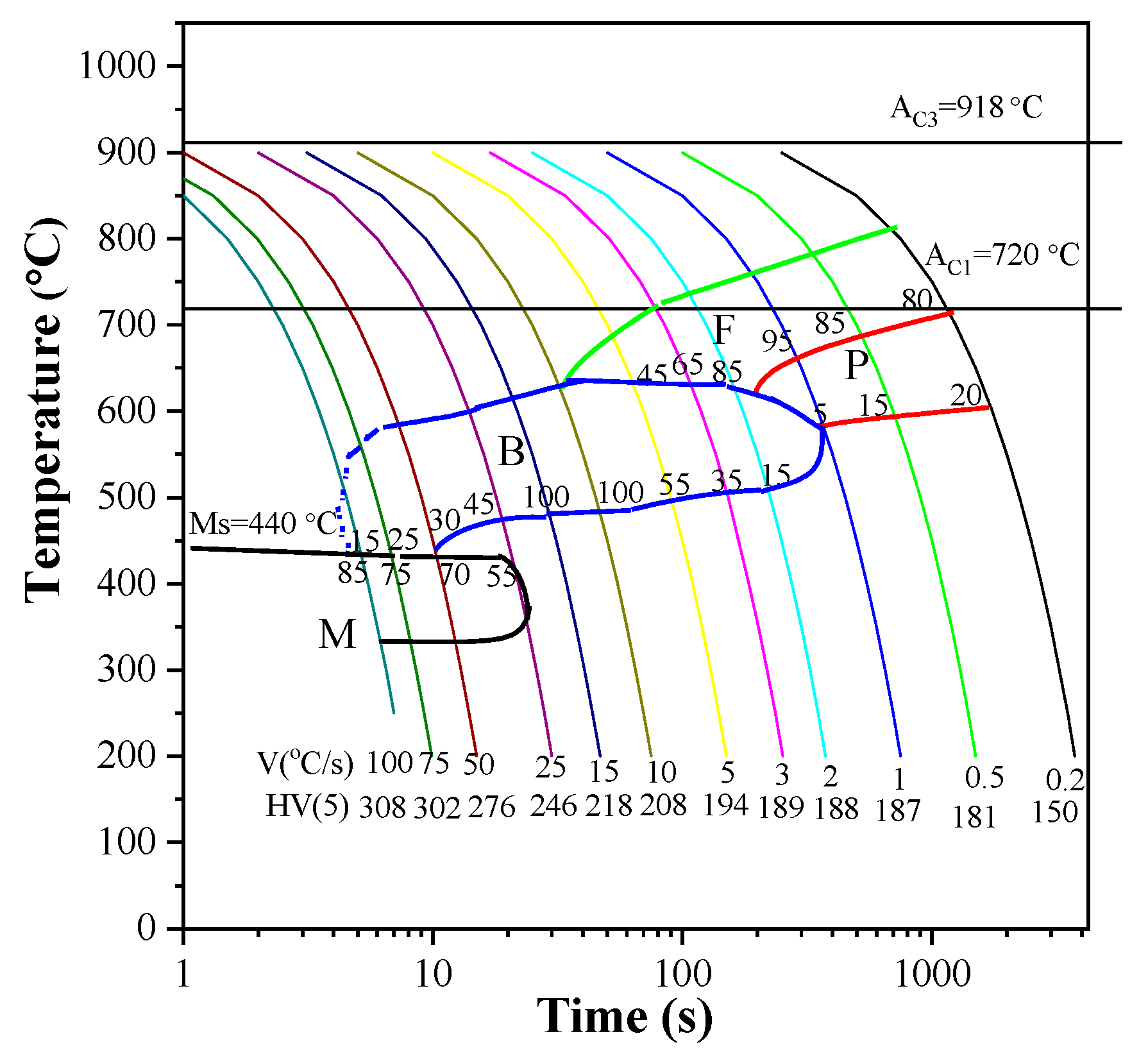
For the second cooling stage, the temperature was allowed to drop freely from 920 K to 200 K. To simulate a wide range of cooling conditions and capture various phase transformations, 12 distinct cooling rates were established, including 100 K/s, 75 K/s, 50 K/s, 25 K/s, 15 K/s, 8.5 K/s, 5 K/s, 3 K/s, 1.67 K/s, 1 K/s, 0.6 K/s, and 0.2 K/s.
iv.
Table 3 presents the cooling rates’ input into the simulation corresponding to various cooling times (t8/5). To align with the actual cooling rates, two-stage cooling rates were selected for input. At higher temperatures, a rapid cooling rate was designated. The heating and comparison data from the simulation experiment are presented in Table 3. The first cooling time is denoted as t1 with a cooling rate of V1; the second cooling time is t2 with a cooling rate of V2; and the total time is represented as t3.
After the thermal simulation, metallurgical examinations were performed on samples subjected to different cooling rates to determine their corresponding microstructures. SH-CCT curves were then derived from these microstructures, with the t8/5 time (cooling interval from 1073 K to 773 K) plotted on the abscissa. The double-wire submerged arc welding (SAW) technique was employed for joining EH36 steel plates, utilizing JW-1 wire and SJ-101 flux (Lincoln Electric Company, Cleveland, OH, USA). Welding experiments were executed with linear energies of 150 kJ/cm, respectively.
Specimens for V-notch Charpy impact testing were extracted at distances of 1 mm, 2 mm, 3 mm, 4 mm, and 5 mm from the fusion line on the fusion-welded steel plates. The low-temperature toughness of the weld metal was assessed using an impact-testing machine (JBW-500, Quanlitest Company, Jinan, China) on V-notch samples with dimensions of 55 × 10 × 10 mm3. The sampling locations for the impact toughness specimens are positioned within 5 mm alongside the weld fusion line, from which five samples are extracted at 1 mm intervals. Both water-cooled Cu backing plates and ceramic backing plates were employed to regulate the post-weld cooling rate of the weldments. Vickers hardness test was conducted on the circular cross-section of the simulated specimens, with three points placed as evenly as possible at the center of the end face. Metallographic samples were prepared at room temperature through mechanically grinding and polishing, followed by etching with a 4% nitric acid alcohol solution, and examined under a metallographic microscope to examine the microstructure evolution at different cooling rates. A thorough statistical analysis of the phase fractions was performed on the optical microscope images of samples acquired at various cooling rates, by utilizing the Image-Pro software version 6.0.

3. Results and Discussions

3.1. Analysis of Thermal Simulation Results

The microstructure evolution in the heat-affected zone at varying cooling rates is experimentally captured and shown in Figure 2. When the cooling rates decrease from 100 K/s to 25 K/s, the predominant microstructures are composed of martensite and bainite. There is a gradual increase in the fraction of bainite as the cooling rate further decreases. With a continued decrease in the cooling rates to 15 K/s, upper bainite, granular bainite, and acicular ferrite start to appear. Ultimately, at a slow cooling rate of 0.2 K/s, the polygonal ferrite and pearlitic phase emerges as the prominent phase.
Based on the analysis of phase constituents and hardness measurements, we derived the Continuous Cooling Transformation (CCT) curve of EH36 steel, as presented in Figure 3. Under conditions of ultrafast cooling, the coarse-grained heat-affected zone (CGHAZ) undergoes a direct transformation into martensite. At a cooling rate of 50 K/s, bainite transformation commences at around 853 K, with the martensitic transformation occurring at 713 K and completing at approximately 513 K, producing the resultant microstructure comprising bainite and martensite. When the cooling rate decreases to 3 K/s, ferrite begins to form at about 973 K, followed by bainite transformation within temperature ranges from 883 K to 769 K. When the cooling rate is decreased to 0.2 K/s, the ferrite has enough time to nucleate and grow, within its transformation spanning 973 K to 1073 K, followed by the pearlite transformation within to 993 K to 863 K.
The analysis of the Vickers hardness value reveals a range of 150 to 310 HV across the extensive range of cooling rates examined. Even under the fastest cooling conditions, the Vickers hardness remains below 350 HV, indicating a low sensitivity to welding-induced cracking. A gradual transition in hardness values is noted as the cooling rate decelerates, with the base steel possessing a hardness of approximately 160 HV. Except for the slowest cooling rate of 0.2 K/s, the hardness values elicited from the simulations generally surpass that of the base steel, indicating that concerns over the softening in the heat-affected zone due to the high heat input from welding is unwarranted.

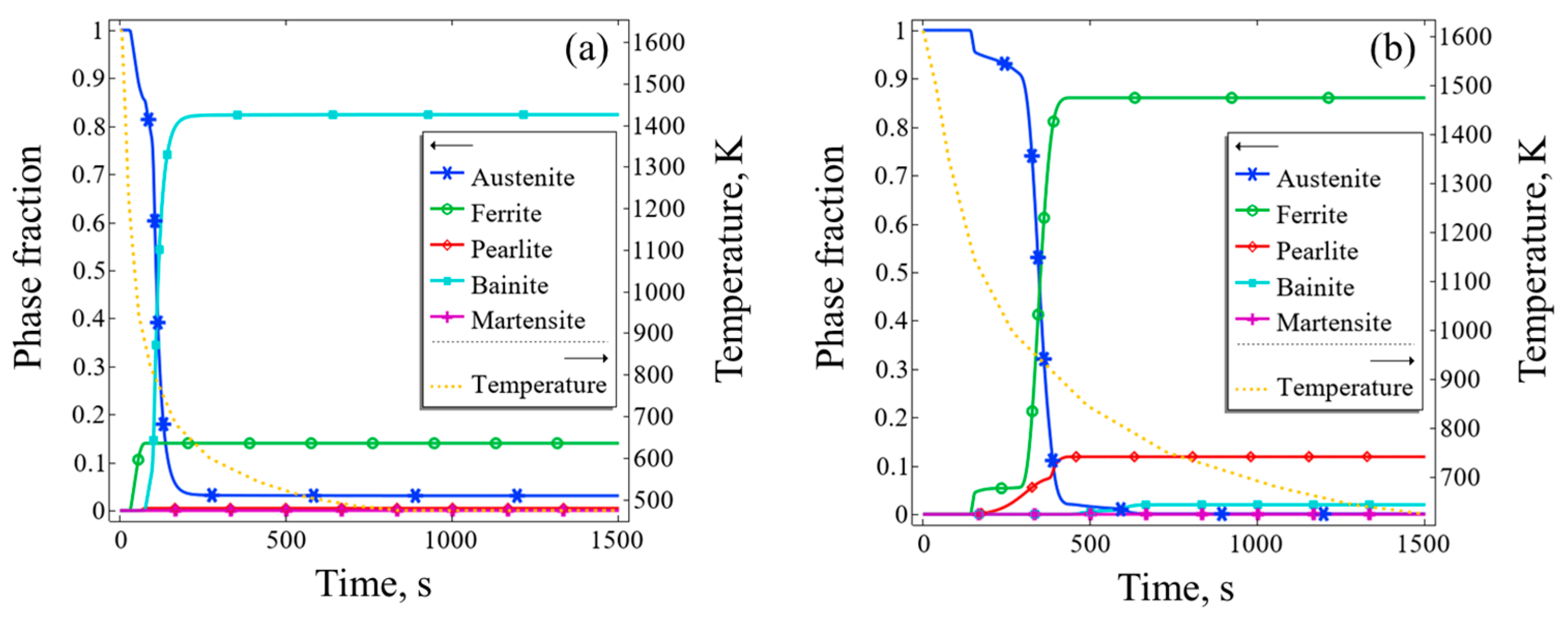
3.2. Validation of the Phase Transformation Model

To estimate the accuracy of the current model that was established on the phase transformation parameters obtained from the SH-CCT curves, we first compare the numerical simulation results and experimental results from Fu et al. [24]. The simulated microstructure evolution under varying temperature histories is shown in Figure 4. With a heat input of 100 kJ/cm, the temperature drops from 1600 K to 480 K over 1500 s, resulting in a microstructure primarily composed of bainite and rest ferrite, without the presence of a martensitic transformation. Increasing the heat input to 250 kJ/cm results in a noticeable shift in the resultant microstructure including primary ferrite and pearlite. This great difference can be ascribed to the lower cooling rate upon a large heat input, which offers enough time for the diffusional ferrite and pearlite transformation, as also confirmed in Figure 2. The quantitative comparison of phase fractions between the simulation and experimental results is presented in Table 4. At both levels of heat input, the predicted values align closely with the empirical data, exhibiting a maximum deviation in the phase fraction of merely 5.5%.

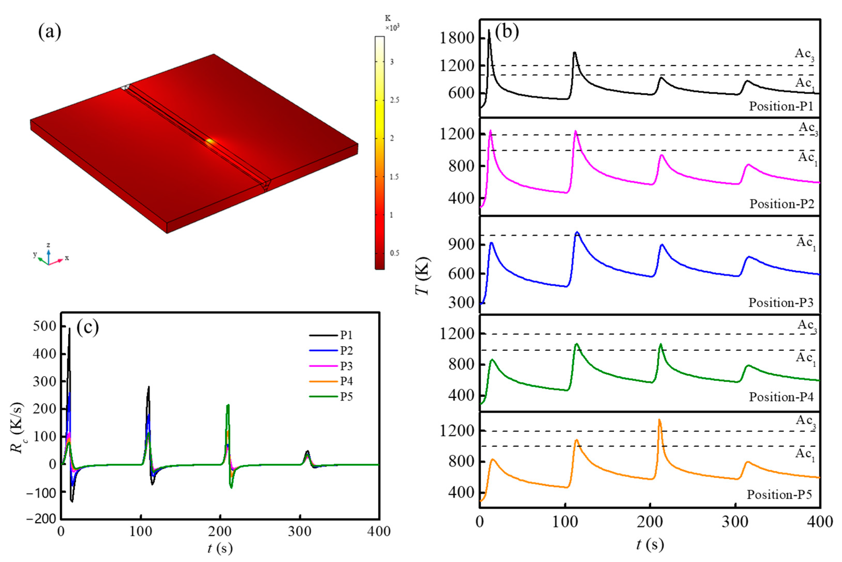
3.3. Temperature Field Distribution

Figure 5a depicts the spatial distribution of the temperature field throughout the model during the third and fourth welding passes. The temperature soars in the molten pool, with the temperature peak over 3000 K. Heat gradually propagates from the molten pool to the heat-affected zone, with the temperature profile being influenced by the divergent paths of the heat source. The temporal temperature profiles at various positions, termed as P1 through P5, are shown in Figure 5b. Point P1 is situated closest to the heat source, reaching a temperature of 2000 K during the initial pass. In the second pass, the thermal peak at P1 diminishes to approximately 1500 K, as the subsequent paths taken by the heat source deviate farther from P1. The other points, though located at more remote distances from the heat source compared to P1, exhibit lower peak temperatures. Nonetheless, they share a similar temperature fluctuation, and all five points display temperature peaks exceeding 800 K, indicating the presence of a phase transformation.
It is imperative that we scrutinize both the heating and cooling rates, as they exert pivotal impacts on the phase transformation kinetics. Figure 5c illustrates the heating and cooling rates at the five points, derived from the time derivative of the temperature. Point P1, located nearest the heat source, reaches the maximum heating and cooling rates of 500 K/s and 120 K/s, respectively. Both the peak heating rate and cooling rate decrease with the increase in the welding pass. The remaining points, lying further from the heat source, exhibit diminished peaks compared to P1, yet follow an analogous pattern of rate modulation. This intense fluctuation in the heating and cooling rate occurs only for a short period when the heat source sweeps over the location. As expected, this repeated thermal cycle strongly affects the phase transformation process.

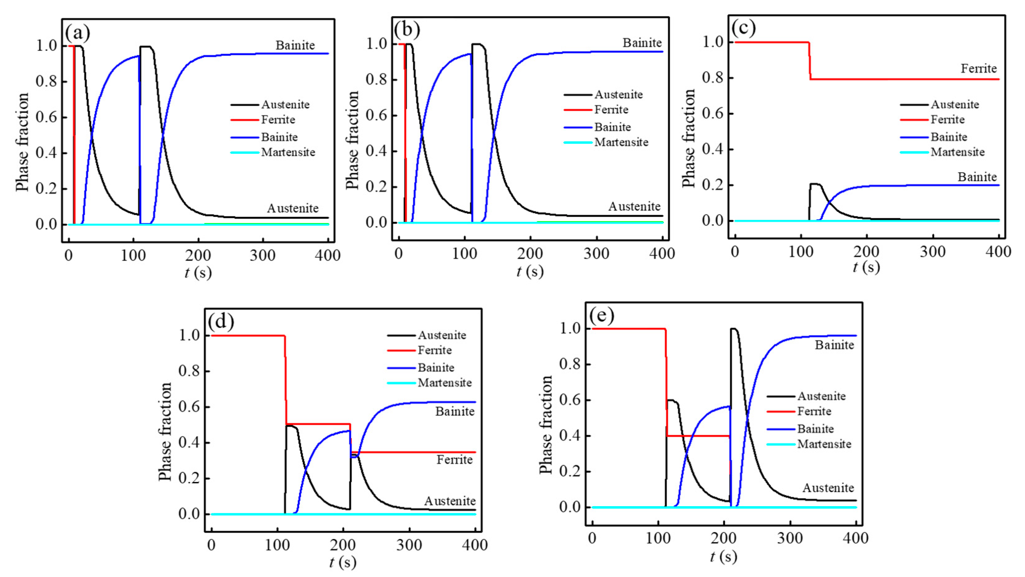
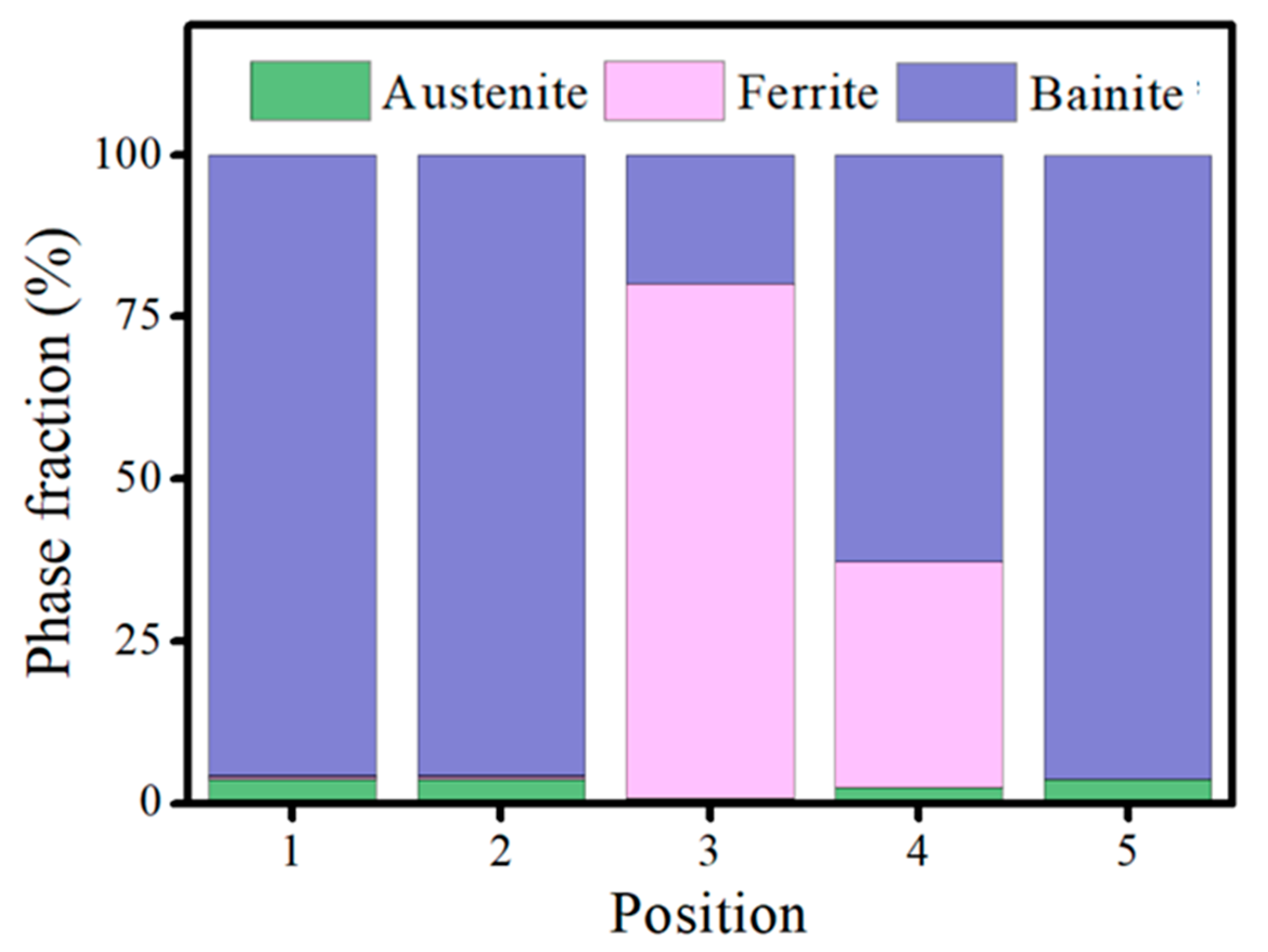
3.4. Microstructure Distribution

Figure 6 shows the microstructure variations at five distinct points within the heat-affected zone throughout the welding process. Points P1 and P2, which are in close proximity to the molten pool during the first two passes, demonstrate a similar pattern of microstructural evolution, as depicted in Figure 6a,b. During the initial two-pass welding (t < 200 s), the heating peak temperature surpasses Ac3, resulting in the transformation of the initial ferrite microstructure into a single austenite phase that subsequently decomposes into bainite upon cooling. P3, with its great distance from the heat source, is subjected to minimal thermal absorption. Only the peak temperature during the second pass reaches 1035 K (Figure 5b), surpassing Ac1. This results in a phase transformation during the second-pass welding, where approximately 20% of the ferrite phase transforms into austenite upon heating, followed by a transformation into bainite during cooling. As for P4, it is far from the heat source of the first pass but near the heat source of the second pass. Therefore, the phase transformation only commences from the second pass of welding, leading to the total generation of approximately 60% bainite during the two consecutive welding steps. However, since the maximum temperature does not reach Ac3, a small amount of the ferrite was retained. However, the temperature reached during the third welding exceeds the Ac3 point, which leads to a final microstructure that is chiefly composed of bainite, with a remaining portion of austenite.
The final phase constituents at the five points are shown in Figure 7. At P1 and P2, it consists of bainite (>95%) and a small amount of austenite. Combined with Figure 6c,d, it can be seen that this is due to the large cooling rate in this region. However, near the starting temperature of Ms, the cooling rate decreases abruptly, preventing the formation of martensite (as is the case at other locations). Due to the low peak temperature at P3, only a few of the base phase is transformed into bainite with a volume fraction of 20%, and the ferrite phase occupies ~80% of the total volume. Along the height z-direction from P3 to P5, close to the weld region, the temperature change is greater, leading to more ferrite converting to austenite during warming. This results in a gradual decrease in ferrite content and a substantial amount of austenite decomposing to bainite during cooling, leading to a gradual increase in bainite content. The above study shows that the region close to the weld primarily consists of bainite with a small amount of residual austenite. In the region away from the weld, it is primarily composed of ferrite and bainite. It should be noted that the final microstructure after cooling is bainite during the multi-pass welding, as led by the high cooling rate.

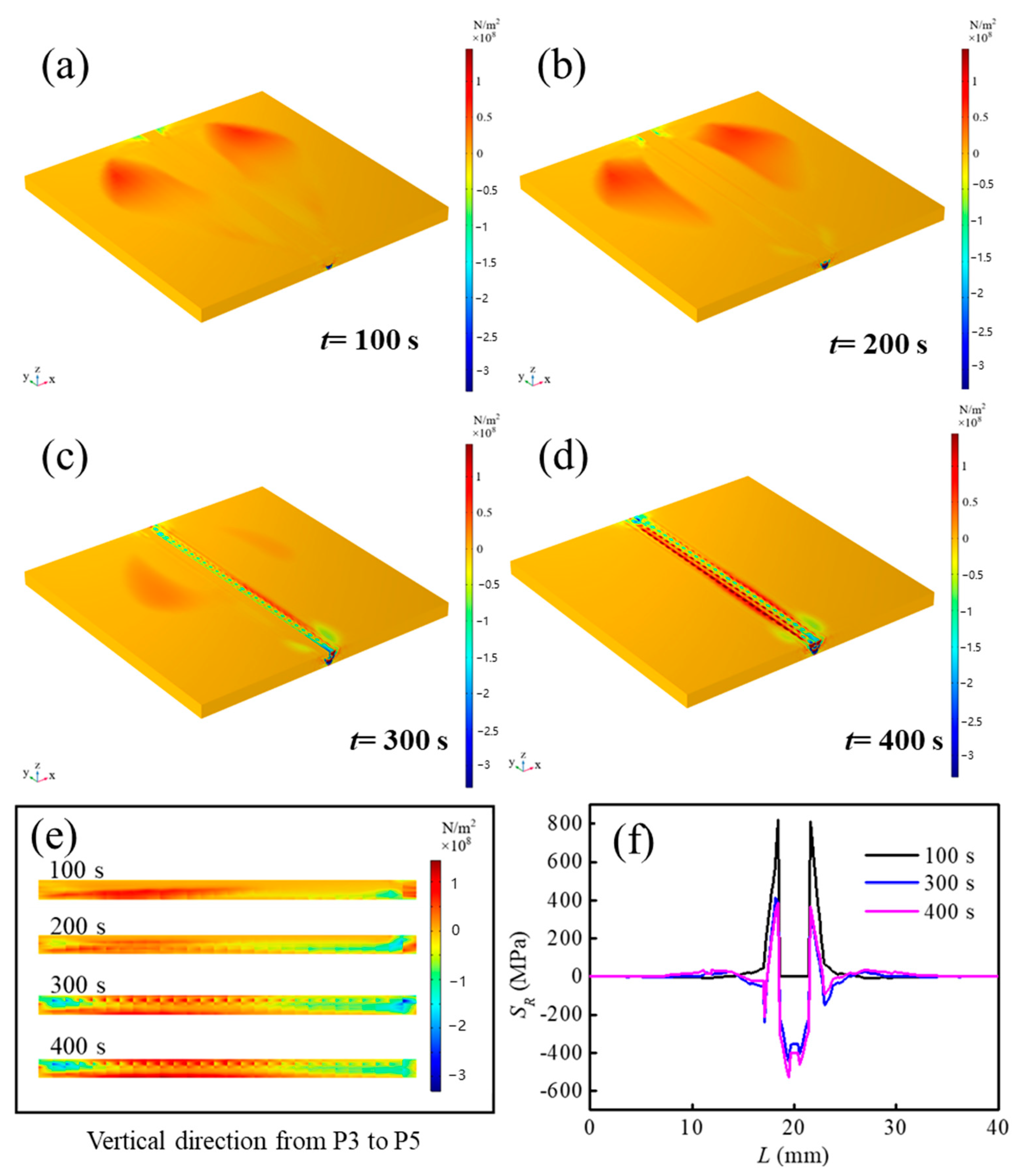
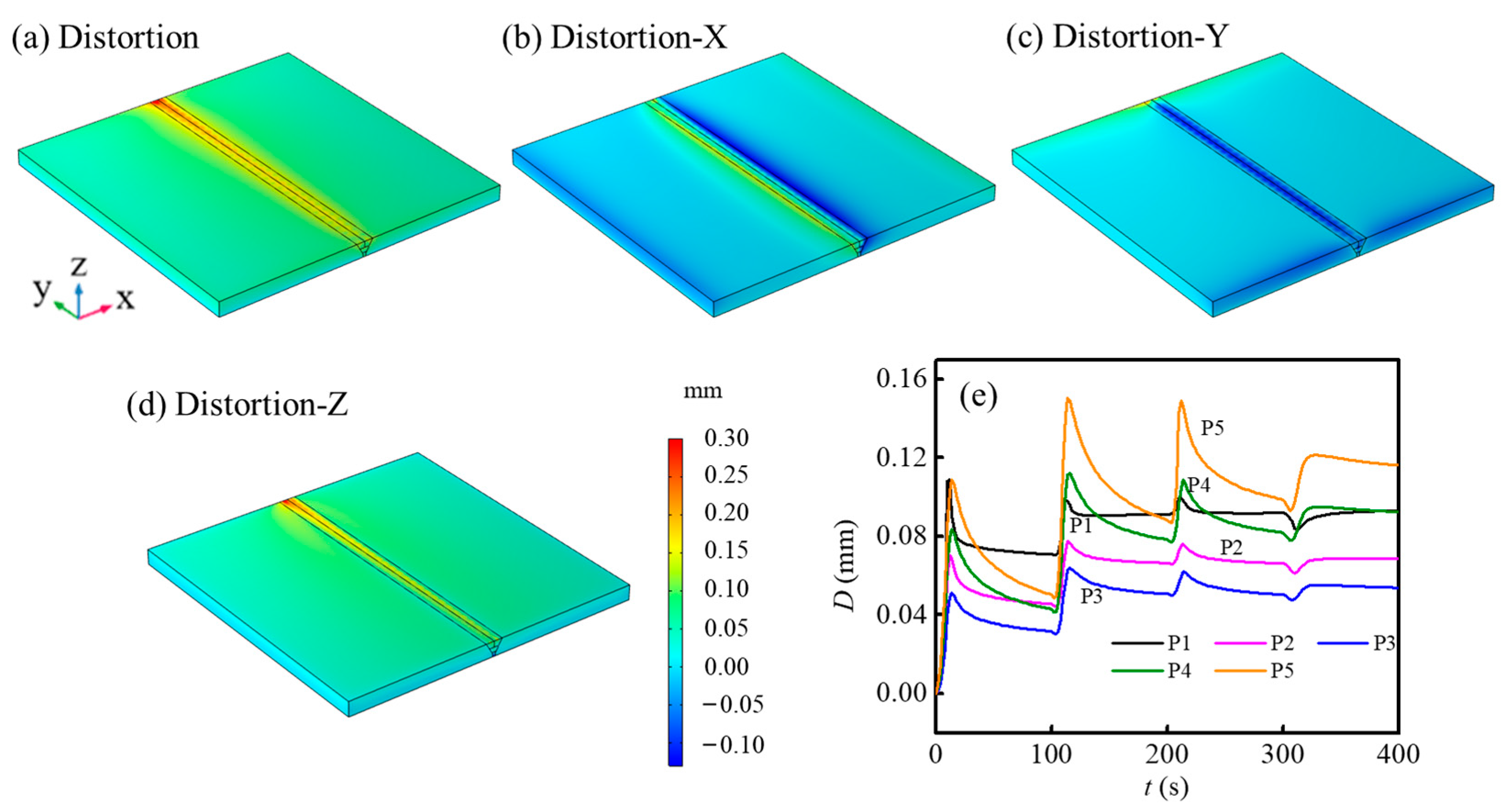
3.5. Residual Stress and Deformation

Figure 8a–d shows the stress distribution of the entire weldment at four different times of 100 s, 200 s, 300 s, and 400 s. It can be seen that, at any stage of welding, the stress in the base material of the weldment is negligible. As the welding progresses, high residual stresses were concentrated in the weld area, with severe stress points concentrated at the fusion line. Meanwhile, partial stress also accumulates in the heat-affected zone outside the weld area. Figure 8e shows the residual stress distribution along the vertical section of the heat-affected zone, located 6 mm away from the center of the weld, captured at various time points. It is clear that there is a large residual stress between consecutive melting pools. Upon completion of the multi-pass welding process, the profile at 400 s indicates a predominant concentration of residual stress at the section center. Figure 8f shows the residual stress distribution on the center intercept line perpendicular to the welding direction. Due to the proximity of the intercepted line segment to the weld of the first pass, the residual stress at 100 s increases significantly compared to the other curves, with the peak of the residual stress reaching 800 MPa. With the increase in time, the peak of the post-weld residual stress curve gradually decreases and is lower than 400 MPa. However, the residual stress trends pertaining to the four passes emulate a coherent trend, with the apogee of residual stress materializing at the periphery of the weld.
The strain in the material induced by multi-pass welding is depicted in Figure 9. Severe deformations in the model are discernible in the Z-axis direction when compared to the strains in the X-axis and Y-axis. The total strain plot bears a striking resemblance to the strain plot along the Z-axis of the model, indicating that the strain in the material is primarily governed by the strain in the Z-axis direction. This phenomenon is attributive to the fixed constraints impeding deformation at the lower surface, thereby constraining thermal expansion and transferring the strain to regions above the Z-axis. Figure 9e demonstrates the strain curves from P1 to P5, with P5 and P4 denoting points that sequentially increase along the Z-axis. The peak value of P5 is 0.15 mm, while the peak value of P4 is 0.11 mm, indicating that the magnitude of the strain gradually increases along the Z-axis direction. P2 and P3 are the two points along the X-axis direction, where the distance from the weld increases successively, with P2 peaking at 0.07 mm and P3 at 0.05 mm. This indicates that the strain diminishes as the distance from the center of the heat source increases.

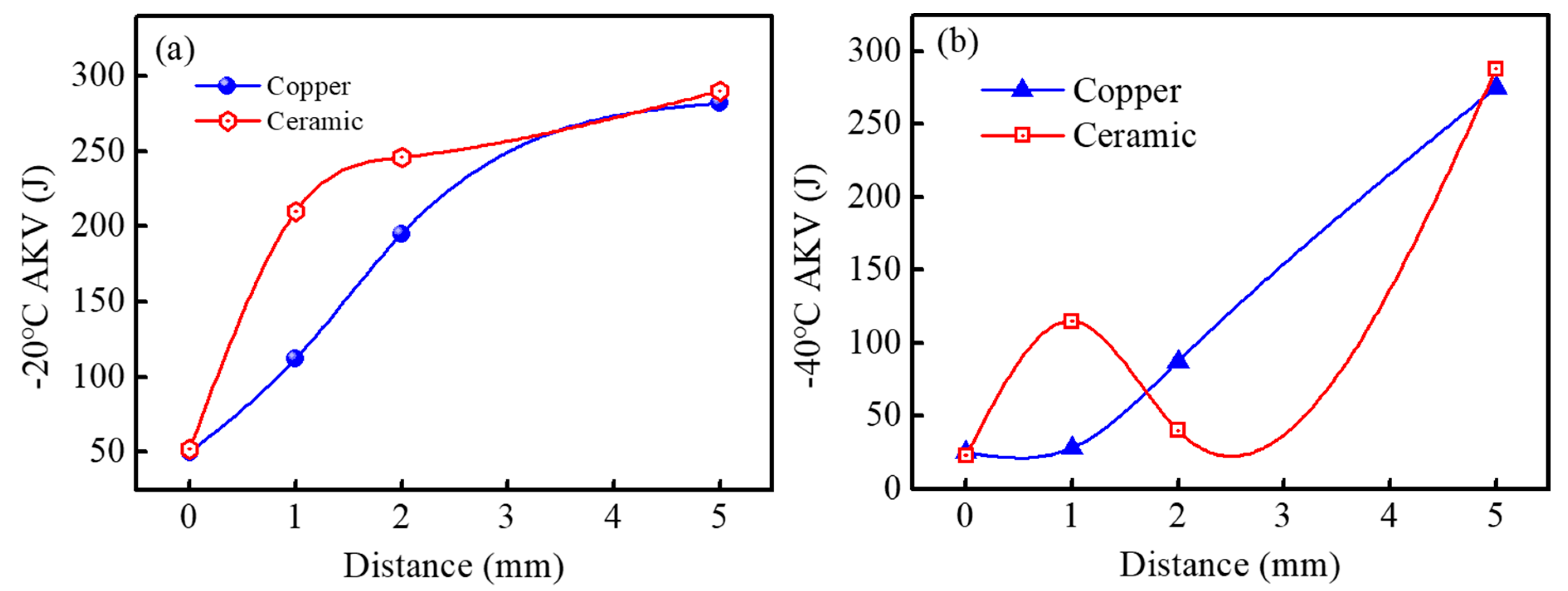
3.6. Impact Performance Test of EH36 Steel

The low-temperature impact performance is critical for the steel used in marine engineering, as it directly affects the safety and reliability of marine engineering structures in low-temperature environments. The cooling rate subsequent to welding exerts a substantial impact on the low-temperature impact toughness of steel, underscoring the need to ascertain an optimal cooling rate when designing the welding process for EH36 steel.
Figure 10 shows the low-temperature impact toughness at various locations on the EH36 steel plate, examined under two different post-welding cooling rates, while maintaining the equivalent line energy. The comparative cooling methods included a water-cooled copper backing plate and ceramic backing plate. Figure 10a shows that the cooling method with ceramic backing slightly surpasses the water-cooled counterpart at 253 K, resulting in an overall higher impact toughness compared to the water-cooled copper backing method. Notably, this improvement is more distinctly emphasized at distances of 1 mm and 2 mm from the weld’s fusion boundary. It can be deduced that reducing the cooling rate is beneficial for improving the low-temperature impact toughness within the heat-affected zone. With the increased distance from the weld pool line, the cooling rate during multi-pass welding gradually decreases, leading to the formation of more acicular ferrite rather than bainite, as shown in Figure 2, Figure 5, Figure 6 and Figure 7, which, in turn, leads to an improvement in impact toughness. A similar phenomenon has been reported in the literature [33]. The dissimilarity in impact toughness attributable to the two cooling modalities at the fusion line and the 5 mm demarcation is negligible, as the toughness in these zones predominantly stems from the interaction between the weld metal and the foundational material. At 233 K, the steel approaches the brittle transition temperature, which leads to a broader scatter in the data, rendering the results less definitive. Additionally, the alleviation of residual stress observed during multi-pass welding and with the increased distance from the fusion line, as depicted in Figure 8, could also contribute to the improved impact toughness.

4. Conclusions

In this study, a finite element model was developed to numerically simulate the complicated evolution of the temperature field and residual stress filed occurring during the multi-pass fusion welding of EH36 steel, elucidating the microstructural transformations and delineating their interconnections with the impact toughness of the welded joints. The key findings are summarized as follows:
  • Throughout the process of multi-pass fusion welding, the peak temperature values and the rate of heating/cooling in the area surrounding the heat source gradually decreases. The absorption of heat consistently reduces in the horizontal direction as the location moves away from the heat source, whereas a potential uptick may occur in the vertical direction owing to the additional heat supplied by subsequent welding passes.
  • The specific parameters of the solid phase transformation model for EH36 steel were confirmed using the experimentally derived SH-CCT curve. Both numerical and experimental findings reveal that multi-pass welding promotes the transformation to bainite in the vicinity of the heat source. Concurrently, an increase in the proportion of acicular ferrite is observed with increasing distance from the welding fusion line in the horizontal plane.
  • The residual stress evolution during the welding process of EH36 revealed that residual stresses are primarily concentrated at the interface between the weld and the heat-affected zone. Maximum residual stresses are predicted near the fusion line at the base of the model, while severe distortion occurs near the fusion line at the top of the model. Furthermore, multi-pass welding may alleviate the residual stress, particularly when coupled with the formation of acicular ferrite during cooling, which results in improved low-temperature impact toughness in areas distant from the heat source. Therefore, this model is intended to facilitate the systematic optimization of the multi-pass welding procedure in forthcoming applications to achieve a more favorable distribution of residual stresses and minimized distortion.

Author Contributions

Methodology, P.W., J.G. and J.W.; software, L.L. and Z.J.; validation, Z.J. and K.F.; formal analysis, J.W. and K.F.; investigation, J.W. and Z.J.; resources, P.W., J.W., L.L. and Z.J.; data curation, K.F.; writing—original draft preparation, P.W. and Z.J.; writing—review and editing, P.W. and L.L.; visualization, Z.J., K.F. and J.G.; supervision, K.F.; project administration, K.F., L.L. and J.G.; funding acquisition, K.F., L.L. and J.G. All authors have read and agreed to the published version of the manuscript.

Funding

This study was funded by the National Natural Science Foundation of China, Grant/Award Numbers: U1860112; and the State Key Laboratory Foundation of University of Science and Technology of Liaoning-Ansteel, Grant/Award Number: HGSKL-USTLN2022-09.

Data Availability Statement

The raw data supporting the conclusions of this article will be made available by the authors on request.

Acknowledgments

The insightful suggestions and technical assistance provided by Wenhua Wu, Shuoshuo Li, Jin Liu, and Qi Liu are also gratefully acknowledged.

Conflicts of Interest

The authors declare no conflicts of interest. Authors J.W. and K.F. were employed by the company State Key Laboratory of Metal Material for Marine Equipment and Application. The remaining authors declare that the research was conducted in the absence of any commercial or financial relationships that could be construed as a potential conflict of interest. The authors declare that this study received funding from State Key Laboratory of Metal Material for Marine Equipment and Application. The funder had the following involvement with the study: State Key Laboratory of Metal Material for Marine Equipment and Application.

References

  1. Corigliano, P.; Crupi, V. Review of Fatigue Assessment Approaches for Welded Marine Joints and Structures. Metals 2022, 12, 1010. [Google Scholar] [CrossRef]
  2. Pranav, N.P.; Sai, B.; Arun, D. Microstructure and mechanical integrity relationship of PDC weld joints involving dissimilar marine grade alloys. J. Manuf. Process. 2020, 50, 111–122. [Google Scholar] [CrossRef]
  3. Wang, D.; Yan, L.; Yin, W.; Zhang, P.; Wang, Z.; Li, G.; Hu, X.; Li, B.; Zhang, W.; Zhu, J. Study on the Tensile and Fatigue Properties of the FH36 Ship Steel Plates at Room and Low Temperatures. Metals 2023, 13, 1563. [Google Scholar] [CrossRef]
  4. Shen, Y.; Liu, S.; Yuan, M.; Dai, X.; Lan, J. Immune Optimization of Double-Sided Welding Sequence for Medium-Small Assemblies in Ships Based on Inherent Strain Method. Metals 2022, 12, 1091. [Google Scholar] [CrossRef]
  5. Verma, J.; Taiwade, R.V. Effect of welding processes and conditions on the microstructure, mechanical properties and corrosion resistance of duplex stainless steel weldments—A review. J. Manuf. Process. 2017, 25, 134–152. [Google Scholar] [CrossRef]
  6. Tsirkas, S.A.; Papanikos, P.; Kermanidis, T. Numerical simulation of the laser welding process in butt-joint specimens. J. Mater. Process. Technol. 2003, 134, 59–69. [Google Scholar] [CrossRef]
  7. Zhang, H.; Wang, Y.; Han, T. Numerical and experimental investigation of the formation mechanism and the distribution of the welding residual stress induced by the hybrid laser arc welding of AH36 steel in a butt joint configuration. J. Mater. Process. Technol. 2020, 51, 95–108. [Google Scholar] [CrossRef]
  8. Zhang, K.; Dong, W.; Lu, S. Finite element and experiment analysis of welding residual stress in S355J2 steel considering the bainite transformation. J. Mater. Process. Technol. 2021, 62, 80–89. [Google Scholar] [CrossRef]
  9. Han, S.W.; Cho, W.; Zhang, L. Coupled simulation of thermal-metallurgical-mechanical behavior in laser keyhole welding of AH36 steel. Mater. Des. 2021, 212, 110275. [Google Scholar] [CrossRef]
  10. Ahmed, M.; El-Sayed Seleman, M.; Touileb, K.; Albaijan, I.; Habba, M.I.A. Microstructure, crystallographic texture, and mechanical properties of friction stir welded mild steel for shipbuilding applications. Materials 2022, 15, 2905–2930. [Google Scholar] [CrossRef] [PubMed]
  11. Ahmed, M.; Abdelazem, K.; El-Sayed Seleman, M.; Alzahrani, B.; Touileb, K.; Jouini, N.; El-Batanony, I.G.; El-Aziz, H.M.A. Friction stir welding of 2205 duplex stainless steel: Feasibility of butt joint groove filling in comparison to gas tungsten arc welding. Materials 2021, 14, 4597–4613. [Google Scholar] [CrossRef] [PubMed]
  12. Albaijan, I.; Ahmed, M.; El-Sayed Seleman, M.; Touileb, K.; Habba, M.I.A.; Fouad, R.A. Optimization of Bobbin tool friction stir processing parameters of AA1050 using response surface methodology. Materials 2022, 15, 6886–6902. [Google Scholar] [CrossRef] [PubMed]
  13. Han, Y.S.; Lee, K.; Han, M.S. Finite Element Analysis of Welding Processes by Way of Hypoelasticity-Based Formulation. J. Eng. Mater. Technol. 2011, 133, 021003. [Google Scholar] [CrossRef]
  14. Chen, M.Y.; Linkens, D.A.; Howarth, D.J.; Beynon, J.H. Fuzzy Model-based Charpy Impact Toughness Assessment for Ship Steels. ISIJ Int. 2004, 44, 1108–1113. [Google Scholar] [CrossRef]
  15. Han, Y. Multiphysics Study of Thermal Profiles and Residual Stress in Welding. Materials 2024, 17, 886. [Google Scholar] [CrossRef] [PubMed]
  16. Li, Y.; Yang, D.; Yang, W.; Wu, Z.; Liu, C. Multiphysics Numerical Simulation of the Transient Forming Mechanism of Magnetic Pulse Welding. Metals 2022, 12, 1149. [Google Scholar] [CrossRef]
  17. Cho, D.W.; Cho, W.I.; Na, S.J. Modeling and simulation of arc: Laser and hybrid welding process. J. Manuf. Process. 2014, 16, 26–55. [Google Scholar] [CrossRef]
  18. Mani, H.; Taherizadeh, A.; Sadeghian, B.; Sadeghi, B.; Cavaliere, P. Thermal–Mechanical and Microstructural Simulation of Rotary Friction Welding Processes by Using Finite Element Method. Materials 2024, 17, 815. [Google Scholar] [CrossRef] [PubMed]
  19. Qi, H.; Pang, Q.; Li, W.; Bian, S. The Influence of the Second Phase on the Microstructure Evolution of the Welding Heat-Affected Zone of Q690 Steel with High Heat Input. Materials 2024, 17, 613. [Google Scholar] [CrossRef] [PubMed]
  20. Yeo, H.; Son, M.; Ki, H. Investigation of microstructure and residual stress development during laser surface melting of AH36 steel using 3-D fully coupled numerical model. J. Heat Mass Transf. 2022, 197, 123366. [Google Scholar] [CrossRef]
  21. Weisz-Patrault, D. Fast simulation of temperature and phase transitions in directed energy deposition additive manufacturing. Addit. Manuf. 2020, 31, 100990. [Google Scholar] [CrossRef]
  22. Ni, J.; Wahab, M.A. A numerical kinematic model of welding process for low carbon steels. Comput. Struct. 2017, 186, 35. [Google Scholar] [CrossRef]
  23. Cho, C.B.; Lee, J.-H.; Lee, C.-H. Distribution and Characteristics of Residual Stresses in Super Duplex Stainless Steel Pipe Weld. Metals 2024, 14, 136. [Google Scholar] [CrossRef]
  24. Fu, J.; El-Fallah, G.M.A.M.; Tao, Q.; Dong, H. A Parameterized Leblond–Devaux Equation for Predicting Phase Evolution during Welding E36 and E36Nb Marine Steels. Materials 2023, 16, 3150. [Google Scholar] [CrossRef] [PubMed]
  25. Winarto, W.; Adhi, P.; Siradj, E.S. Effects of Heat Input on Microstructures, Hardness, and Residual Stress of GMA Weld Dissimilar butt joints between Stainless Steel SUS 316 and Marine Steel AH 36. ISIJ Int. 2020, 38, 182–185. [Google Scholar] [CrossRef]
  26. Zubairuddin, M.; Albert, S.; Vasudevan, M. Numerical simulation of multi-pass GTA welding of grade 91 steel. J. Manuf. Process. 2017, 27, 87. [Google Scholar] [CrossRef]
  27. García-García, V.; Mejía, I.; Reyes-Calderón, F. Thermo-mechanical-microstructural simulation of double-pass welding process in a TWIP steel by FE formulation and probabilistic model. Int. J. Adv. Manuf. Technol. 2020, 111, 1115–1134. [Google Scholar] [CrossRef]
  28. Maekawa, A.; Kawahara, A.; Serizawa, H. Fast three-dimensional multipass welding simulation using an iterative substructure method. J. Mater. Process. Technol. 2015, 215, 30–41. [Google Scholar] [CrossRef]
  29. Mostafa, J.; Reza, T.; Ammar, M.M. Using double ellipsoid heat source model for prediction of HAZ grain growth in GTAW of stainless steel 304. Mater. Today Commun. 2022, 31, 103411. [Google Scholar] [CrossRef]
  30. Mi, G.; Xiong, L.; Wang, C. A thermal-metallurgical-mechanical model for laser welding Q235 steel. J. Mater. Process. Technol. 2016, 238, 39–48. [Google Scholar] [CrossRef]
  31. Genchev, G.; Dreibati, O.; Ossenbrink, R. Physical and Numerical Simulation of the Heat-Affected Zone of Multi-Pass Welds. Mater. Sci. Forum. 2013, 762, 544–550. [Google Scholar] [CrossRef]
  32. Chandrappa, N.; Bernacki, M. A level-set formulation to simulate diffusive solid/solid phase transformation in polycrystalline metallic materials—Application to austenite decomposition in steels. Comput. Mater. Sci. 2023, 216, 111840–111855. [Google Scholar] [CrossRef]
  33. Jorge, J.; De Souza, L.; Mendes, M.; Bott, I.; Araújo, L.; Santos, V.; Rebello, J.; Evans, G. Microstructure characterization and its relationship with impact toughness of C–Mn and high strength low alloy steel weld metals—A review. J. Mater. Res. Technol. 2021, 10, 471–501. [Google Scholar] [CrossRef]
Figure 1. The illustration of geometrical model.
Metals 14 00476 g001
Figure 2. Microstructure morphology at several typical cooling rates (B: Bainite, F: Ferrite; P: Pearlite; M: Martensite).
Metals 14 00476 g002
Figure 3. Continuous heating and cooling curves in the heat-affected zone of welding (SH-CCT).
Metals 14 00476 g003
Figure 4. Microstructure evolution as a function of time at different welding energy densities: (a) 100 kJ/cm, and (b) 250 kJ/cm.
Metals 14 00476 g004
Figure 5. Temperature field distribution during multi-pass welding process: (a) 250 s and (b) 350 s spatial distribution of temperature, and (c) temperature at different locations over time.
Metals 14 00476 g005
Figure 6. Microstructure evolution at different locations: (a) P1, (b) P2, (c) P3, (d) P4, and (e) P5.
Metals 14 00476 g006
Figure 7. Fraction of phases at different positions at the end of welding.
Metals 14 00476 g007
Figure 8. Regulation of residual stress by multi-pass welding: the three-dimension residual stress evolution at multi-pass welding time periods of (a) 100 s, (b) 200 s, (c) 300 s, and (d) 400 s; (e) residual stress distribution in the vertical section of the heat-affected zone; (f) residual stress distribution on special line segments.
Metals 14 00476 g008
Figure 9. Effect of multi-pass welding on material distortion: material at 400 s: (a) total distortion, (b) X-direction, (c) Y-direction, (d) Z-direction, and (e) distortion at positions P1 to P5 versus time.
Metals 14 00476 g009
Figure 10. Effect of cooling rate on the impact toughness of multi-pass weldments under different temperatures: (a) impact energy at 253 K (−20 °C); (b) impact energy at 233 K (−40 °C).
Metals 14 00476 g010
Table 1. The employed thermophysical parameters at various temperatures for EH36 steel, Reprinted from ref. [26].
Temperature (K)Density (kg/m3)Thermal Conductivity (W/m·K)Specific Heat (J/kg·K)Poisson’s RatioYoung’s Modulus (GPa)
298783045.744500.29196.38
373781045.884800.293191.06
473778045.025200.297182.09
573774043.165600.301172.98
673771040.625700.305163.74
773767037.795800.308154.36
873764035.055900.312144.83
973760032.376000.318137.74
1073758029.666050.327125.86
1173754227.776100.346115.47
1273750528.986300.352105.45
1473743031.386600.36485
1673732033.86900.37659
1753725034.611420--
1773721034.681120--
1793698033.74820--
3273698033.74820--
Table 2. The chemical composition of EH36 test steel (wt.%).
ElementCSiMnNAlTiSPNbFe
wt.%0.090.381.430.00240.0290.0140.0030.0140.025Rest
Table 3. Comparing heating in the simulation experiment.
Serial Numbert8/5 (s)t1 (s)V1 (K/s)t2 (s)V2 (K/s)t3 (s)
1341007.210011.2
24.5410010.67514.6
36410014.45018.4
4124100292533
5204100481552
6354100858.589
76041001445148
810041002403244
918041004311.67435
1030041007201724
11500410012000.61204
121500410036000.23604
Table 4. Comparison of experimentally determined and model-predicted phase fractions.
Phase Fraction (%)Heat Input (100 kJ/cm)Heat Input (250 kJ/cm)
ExperimentSimulationExperimentSimulation
Ferrite 12.114.085.986.0
Pearlite00.514.111.9
Bainite87.982.402.1
Austenite03.100
Disclaimer/Publisher’s Note: The statements, opinions and data contained in all publications are solely those of the individual author(s) and contributor(s) and not of MDPI and/or the editor(s). MDPI and/or the editor(s) disclaim responsibility for any injury to people or property resulting from any ideas, methods, instructions or products referred to in the content.

